DOI:10.32604/cmc.2021.015326
| Computers, Materials & Continua DOI:10.32604/cmc.2021.015326 | |
| Article |
Machine Learning Techniques Applied to Electronic Healthcare Records to Predict Cancer Patient Survivability
1eVIDA Lab, University of Deusto, Bilbao, 48007, Spain
2Success Clinic Oy, Helsinki, 00180, Finland
*Corresponding Author: Ornela Bardhi. Email: ornela.bardhi@deusto.es
Received: 15 November 2020; Accepted: 06 February 2021
Abstract: Breast cancer (BCa) and prostate cancer (PCa) are the two most common types of cancer. Various factors play a role in these cancers, and discovering the most important ones might help patients live longer, better lives. This study aims to determine the variables that most affect patient survivability, and how the use of different machine learning algorithms can assist in such predictions. The AURIA database was used, which contains electronic healthcare records (EHRs) of 20,006 individual patients diagnosed with either breast or prostate cancer in a particular region in Finland. In total, there were 178 features for BCa and 143 for PCa. Six feature selection algorithms were used to obtain the 21 most important variables for BCa, and 19 for PCa. These features were then used to predict patient survivability by employing nine different machine learning algorithms. Seventy-five percent of the dataset was used to train the models and 25% for testing. Cross-validation was carried out using the StratifiedKfold technique to test the effectiveness of the machine learning models. The support vector machine classifier yielded the best ROC with an area under the curve
Keywords: Machine learning; EHRs; feature selection; breast cancer; prostate cancer; survivability; Finland
One in three people in Finland will develop cancer at some point during their lifetime [1]. Every year, about 30,000 people are diagnosed with cancer. However, only two-thirds will recover from the disease [1]. The most common cancer in men in Finland is prostate cancer (PCa) [2]. In 2018, 5,016 new PCa cases were detected in Finland [3]; 28% of all new cancers in men. In the same year, 914 men died of PCa, with age-standardized mortality standing at 11.2 per 100,000. PCa patient mortality has remained relatively constant in recent years. By the age of 80, a Finnish man has an 11.6% risk of developing and 1.6% risk of dying from prostate cancer. The most substantial identified risk factors are age, ethnic background, hereditary susceptibility and environmental factors. Approximately 2%–5% of prostate cancers relate to hereditary cancers, and about 15%–20% are familial [4–6]. A twin Scandinavian study showed that environmental factors play a more significant role in the development of PCa than hereditary factors [7]. Excessive consumption of fat, meat and multivitamins may be associated with increased PCa risk [8,9]. Exercise has been found to reduce PCa risk [10]. Smoking, on the other hand, appears to increase aggressive PCa risk and may also increase its progression [11].
The relative PCa survival rate one year after diagnosis is 98%: and after five years, 93%. PCa prognosis has remained unchanged over the last ten years [3]. The 10-year survival forecast for men with local, highly differentiated prostate cancer is the same regardless of treatment (90%–94%). Treatments include active monitoring and, if necessary, radical treatments (surgery or radiotherapy), conservative monitoring and, where needed, endocrine therapy [2].
The most common cancer in women in Finland is breast cancer (BCa). In 2018, 4,934 new BCa cases were detected in Finland; 29.8% of all new cancers in women. In the same year, 873 women died of BCa, with age-standardized mortality standing at 12.2 per 100,000 [3]. BCa patient mortality has remained relatively constant in recent years. By the age of 70, a Finnish woman has an 8.52% risk of developing BCa. The relative BCa survival rate one year after diagnosis is 97.6%: and after five years, 91%. BCa prognosis has slightly improved over the last 15 years [3]. Among the identified risk factors are gender, age, family history and hereditary susceptibility, ethnicity, pregnancy and breastfeeding history, weight, alcohol consumption and inactivity. The twin Scandinavian study [7] mentioned above showed that environmental factors play a far more significant role in BCa development than hereditary factors. Only 27% risk can explain hereditary factors [7]. It is worth noting that male breast cancer accounted for just 0.6% of all Finnish BCa in 2018 [3], and treatment protocol is mainly based on the principles for female BCa [12].
Different drugs are currently in use to treat BCa and PCa, and new ones are frequently being clinically trialed. Such treatments include chemotherapy, radiotherapy, endocrine therapy, surgery and, more recently, targeted therapy and immunotherapy. These treatments are administered in combination with each other to cure or keep the disease at bay.
Previous studies have been conducted on predicting the risk of developing BCa and PCa. However, they differ substantially with regard to the different type of information used to make such predictions. In the case of BCa risk prediction, [13] machine learning (ML) models were developed using Gail model [14] inputs only, and models using both Gail model inputs and additional personal health data relevant to BCa risk. Three out of six of the ML models performed better when the additional personal health inputs were added for analysis, improving five-year BCa risk prediction [13]. Another study assessed ML ensembles of preprocessing methods by improving the biomarker performance for early BCa survival prediction [15]. The dataset used in this study consisted of genetic data. It concluded that a voting classifier is one way of improving single preprocessing methods. In [16], the authors developed an automated Ki67 scoring method to identify and score the tumor regions using the highest proliferative rates. The authors stated that automated Ki67 scores could contribute to models that predict BCa recurrence risk. As in [15], genetic inputs, pathologic data and age were used to make predictions.
In the case of PCa risk predictions, Sapre et al. [17] showed that microRNA profiling of urine and plasma from radical prostatectomy could not predict if PCa is aggressive or slow-growing. Besides RNA data, clinical and pathological data were used to train and test ML. The authors of [18] added the PCa gene 3 biomarker to the Prostate Cancer Prevention Trial risk calculator (PCPTRC) [19], thereby improving PCPTRC accuracy. Reference [20] is an updated version of the PCPTRC calculator. A recent study in the USA on utilizing neighborhood socioeconomic variables to predict time to PCa diagnosis using ML [21] showed that such data could be useful for men with a high risk of developing PCa.
This paper presents the results of a study that included Electronic Healthcare Records (EHRs) of breast and prostate cancer patients in a region in Southwest Finland. EHRs are the systematized collection of electronically-stored patient and population health information in digital format. Information stored in such systems varies from demographic information to all types of treatments and examinations that patients undergo throughout the course of their care. This information usually lacks structure or order, and requires thorough data cleaning prior to conducting any meaningful analysis. The social impact of analyzing such data is enormous. Understanding the most important variables for a particular disease helps hospitals allocate resources, and also helps healthcare professionals individualize care pathways for each patient. Patients thus benefit from a better quality of life. This study aimed to determine the most critical variables impacting BCa and PCa patient survivability, and how the use of ML models can aid prediction.
This paper complies with the GATHER statement [22].
A retrospective cohort study was conducted using the EHRs of BCa and PCa patients treated at the District of Southwest Finland Hospital, via the Turku Centre for Clinical Informatics (TCCI). TCCI provided the Data Analytics Platform (DAP), a remote server where data was accessed and analyzed via a secure shell (SSH) connection.
No ethical approval was required. Nonetheless, it was necessary to apply for authorization to use the data in compliance with privacy and ethical regulations under Finnish law. This study included anonymized patient data only.
Success Clinic Oy sponsored the database.
The BCa and PCa data was stored in a PostgreSQL database engine in 24 separate tables according to treatment, or the department where the information was collected in the hospital. Structured Query Language (SQL) was utilized to retrieve data for each treatment line (e.g., chemotherapy, radiotherapy, etc.) for both cancers separately and then each file was stored in CSV format. This approach was selected because the data was unstructured and thorough data cleaning and preprocessing conducted prior to analysis. In total, there were 20,006 individual patients aged 19–103, of whom 9,998 were female and 10,008 male. Of 20,006 patients, 9,922 were diagnosed with prostate cancer and 10,113 with breast cancer; 115 were male, 86 of whom were diagnosed with breast cancer only. The database contains information dating from January 2004 (when the regional repository was initially created) until the end of March 2019.
The variables collected in this study were primarily based on previous research [23], a mixed-method study was conducted aimed at understanding breast and prostate cancer patients’ care journey from their perspective. The data in [23] was collected using qualitative methods and EHRs. Hospitals, however, do not collect the kind of data retrieved through qualitative methods in their electronic healthcare systems. An explanation of the type of data available and retrieved from the TCCI is given below.
Demographic data included the patient’s current age, age at diagnosis, date of birth, date of death and years suffering from cancer from the first date of diagnosis. Although patient residence details were collected as part of the study, they did not form part of the analysis.
Medical data included biopsy results: cancer type, grade, Gleason score, progesterone receptor score, estrogen receptor score, HER2 receptor score, tumor size, lymph node involvement, Prostate-Specific Antigen (PSA). Treatment lines included chemotherapy drugs, number of cycles, chemotherapy start and finish date; the number of radiotherapy sessions, doses delivered, fractions delivered, radiation treatment start and finish date; endocrine therapy drugs; targeted therapy drugs; bisphosphonate drugs; comorbidities at the time of data collection.
The World Health Organization International Classification of Diseases (ICD) version 10 [24] codes were employed for each disease. The main categories for BCa ICD10 codes were used such as c50, c50.1, c50.2, c50.3, c50.4, c50.5, c50.6, c50.7, c50.8 and c50.9. This was done because there were some inconsistencies when associating male breast cancer with male patients. Some were stored as being diagnosed with female breast cancer. This variable was dropped for PCa as there is only one ICD10 code–c61. Grade categories were grade 1, grade 2 and grade 3, and the Gleason score was 6 to 10. There were 18 separate categories for tumor size and 15 for lymph node involvement. Anatomical Therapeutic Chemical (ATC) Classification System codes were used to code chemotherapy, endocrine therapy, targeted therapy and bisphosphonate drugs.
Lifestyle data included smoking and alcohol consumption. Other information such as diet, exercise, family history or female nulliparity [25] was not initially collected by hospitals, and is therefore not included in this study. Participant demographic characteristics are shown in Tab. 1, created using tableone [26], a Python library for creating patient population summary statistics.
Table 1: Patient characteristics grouped according to gender

Machine learning methods were employed for both feature selection and classification. Python (version 3.5.2) [27] programming was used to preprocess and analyze data utilizing Python libraries. Besides Python, SQL was used since data was stored in a PostgreSQL server. The main libraries used during the preprocessing stage were Pandas and NumPy, both of which are open-source libraries providing high-performance, easy-to-use data structures and data analysis tools for scientific computing. Matplotlib and Seaborn open-source data visualization libraries were also used. The study used the scikit-learn (sklearn) library [28] for machine learning analysis, and was conducted on the server provided by TCCI.
Most of the variables were categorical. Hence one-hot encoding was utilized for encoding and preparing data for ML analysis. This is due to the fact that machine learning models do not work with categorical variables.
Train_test_split( ), a pre-defined method in the sklearn library, was employed to train and test the models. 75% of the dataset was used for training the models and 25% for testing. The stratify parameter was included to split the data in a stratified fashion using the desired variable to predict survivability as class labels.
The effectiveness of nine machine learning classifiers was assessed when predicting the probabilities that individuals were likely to survive or die within the first 15 years of diagnosis. The nine classifier types were: logistic regression (LR), support vector machine (SVM), nearest neighbor, naïve Bayes (NB), decision tree (DT), and random forest (RF). These machine learning models were selected because each model has significant advantages, which could make it the best model to predict survivability/mortality risk based on the inputs chosen during the feature selection stage.
Logistic regression classifies data by using maximum likelihood functions to predict the probabilities of outcome classes [29] such as alive/dead, healthy/sick, etc. LRs are widely used because they are simple and explicable. In order to model nonlinear relationships between variables with logistic regression, the relationships must be found prior to training, or various transformations of variables performed [30].
Support vector machines were first introduced by Cortes et al. [31]. Their objective is to find a hyperplane in the N number feature space that maximizes the distance between points corresponding to training dataset subjects in the output classes [32]. SVMs are generalizable to different datasets and work well with high-dimensional data [29] and can accurately perform linear and nonlinear classification. Nonlinear classification is performed using the kernel, which maps inputs into high-dimensional feature spaces. However, SVMs require a lot of parameter tuning [13,29,33].
Nearest neighbor algorithms work by finding a preset number of training samples that are closest in distance to the new point, and later predict the labels [34]. In k-nearest neighbor (KNN) learning, the number of samples is a user-defined constant. By contrast, in radius-based neighbor learning, the constant varies depending on the local density of points [33]. Despite their simplicity, nearest neighbors have been successful in many classification and regression problems. As a non-parametric method, it often manages to classify situations where the decision boundary is highly irregular.
Naive Bayes models, unlike the previously described classifiers, are probabilistic classifiers [29] based on the Bayes theorem. NB models generally require less training data and have fewer parameters compared to other models such as SVMs etc. [35]. NB models are good at disregarding noise or irrelevant inputs [35]. However, they consider that the input variables are independent, which is not valid for most classification applications [29]. Despite this assumption, these models have been successful in many complex problems [29].
Decision trees organize knowledge extracted from data in a recursive hierarchical structure composed of nodes and branches [36]. DTs are non-parametric, supervised learning methods used for both classification and regression, whose goal is to create a model that predicts the value of a target feature by learning simple rules inferred from the input features. Besides nodes and branches, DTs are made up of leaves, the last nodes being found at the bottom of the tree [32]. Some advantages of DTs are that they are simple to understand and interpret (trees can be visualized), require scarce data preparation (no data normalization is needed), can handle both numerical and categorical data, and the model can be validated by using statistical tests [33]. Besides all these positive aspects of DTs, particular care should be taken when working with them as over-complex trees can be created that are poorly generalized [33]. DTs can also be unstable when introducing small variations into data, which can be mitigated by using them within an ensemble [33].
Random forest is a meta model that fits various decision tree classifiers into a number of sub-samples on the dataset. RF uses averaging to improve predictive accuracy and control overfitting. The sub-sample size is controlled by the max_sample parameter when the bootstrap is set to True (default); otherwise, each tree uses the whole dataset. Individual DTs generally tend to have high variance and overfit. RFs yield DTs and take an average of the predictions, which leads to some errors being canceled out. RFs achieve reduced variance by combining diverse trees, sometimes to the detriment of a slight increase in bias. In practice, variance reduction is often significant, hence yielding a better overall model.
The LR, NB, DT, SVM, and KNN models were implemented using the Python scikit-learn package (version 0.23.1) [28,33]. The “linear_model.LogisticRegression” function was used for logistic regression, and “naive_bayes.GaussianNB” and “naive_bayes.BernoulliNB” for naive Bayes. The “tree.DecisionTreeClassifier” function was used to create a decision tree, and “ensemble.RandomForestClassifier” to create a random forest classifier. “svm.SVC” implementation was applied with probability predictions enabled, and “svm.LinearSVC” for the support vector machine. The “neighbors.KNeighborsClassifier” model was used for nearest neighbor, and a grid search technique to extract the best parameters for each function.
Finally, all the features/variables used to train the machine learning models were scaled to be centered around 0 and transformed to unit variance since the datasets had features on different scales, e.g., height in meters and weight in kilograms. Rescaling variables is mandatory because machine learning models assume that data is normally distributed. Also, doing so helps to train the models quickly and generalize more effectively [37]. StandardScaler was chosen to scale the data since it is one of the most popular rescaling methods [37].
This section is structured in two parts. The first explains feature selection, and the second addresses the classification analysis performed in relation to the features selected from part one.
Feature selection is the process of selecting a set of variables that are significant to the analysis to be conducted. The objective of feature selection is manifold: (i) it provides a better understanding of the underlying process generating data, (ii) faster and more cost-effective predictors, and (iii) improves predictor prediction performance [38].
There are different techniques to select the relevant variables. The first technique employed was recursive feature elimination (RFE), whose goal is to remove features step-by-step by using an external estimator that assigns weights to features [33]. The estimator is trained on the initial dataset, which contains all the features. Each feature’s importance is obtained via two attributes: (i) coef_; or (ii) feature_importances_ [33]. The least important features are eliminated from the current set of features recursively until the set number of features to be selected is reached. The estimators used to perform RFE are logistic regression, stochastic gradient descent, random forest, linear SVM and perceptron. Tab. 2 shows the estimators used in analysis and accuracy for each number of features selected when predicting whether a patient will survive.
Table 2: Feature selection algorithms and accuracy score

Besides RFE, SelectFromModel with a Lasso estimator was used. SelectFromModel is a meta-transformer used alongside an estimator. After fitting, the estimator has an attribute stating feature importance, such as the coef_or feature_importances_attributes. In order to control the feature selection algorithms, the same parameters were used to set a limit on the number of features to be selected, the n_features_to_select for RFE and max_features for SelectFromModel.
In order to verify the results obtained from RFE and the SelectFromModel algorithms, the Random Forest Classifier and XGBoost [39] were used. Both these algorithms have a specific attribute to select the best features. The feature_importances_attribute was used for the Random Forest Classifier and the plot_importance( ) [39,40] method for XGBoost with height set to 0.5 as the parameter. XGBoost was employed on the basis of being an optimized distributed gradient boosting library designed to be flexible, efficient, and portable [39]. It uses machine learning algorithms under the Gradient Boosting framework as well as providing parallel tree boosting, which has proven to be highly efficient at solving various problems.
The XGBoost results with the most important features and scores are shown in Fig. 1. In total, 21 features were selected after running the XGBoost estimator for BCa data, and 15 features for PCa data. The results from Random Forest are shown in Tab. 3. All features selected by the algorithms are shown for both BCa and PCa.

Figure 1: Feature selection and importance extracted from XGBoost for (a) breast cancer and (b) prostate cancer. Features for both databases are specific to the diseases, and indexes for each feature are different, ex. f0 in the breast cancer dataset represents feature c50_diag_age, whereas in prostate cancer, it represents c61_diag_age, etc.
Table 3: Features selected using different estimators for breast cancer

Apart from the features shown in Tab. 3, there are six more features (total 21) that were selected but not shown in the table: her2_neg, alcohol_no, alcohol_yes, L02BG04, tumor_size_1, lymph_node_0. All features mentioned above had an F score of at least 1, also shown in Fig. 2. All feature indexes refer to the features themselves when shown in Tabs. 3 and 4.
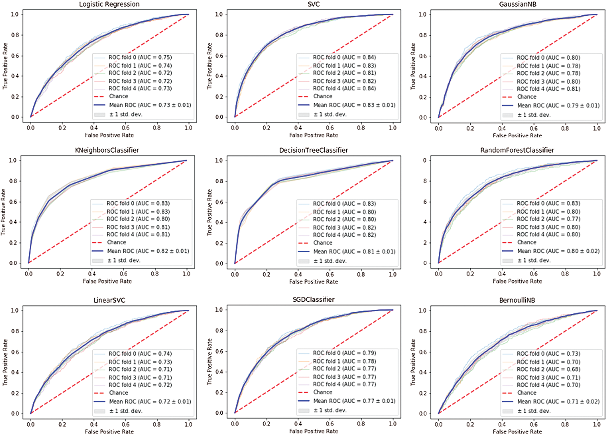
Figure 2: ROC AUC for breast cancer
Table 4: Features selected using different estimators for prostate cancer

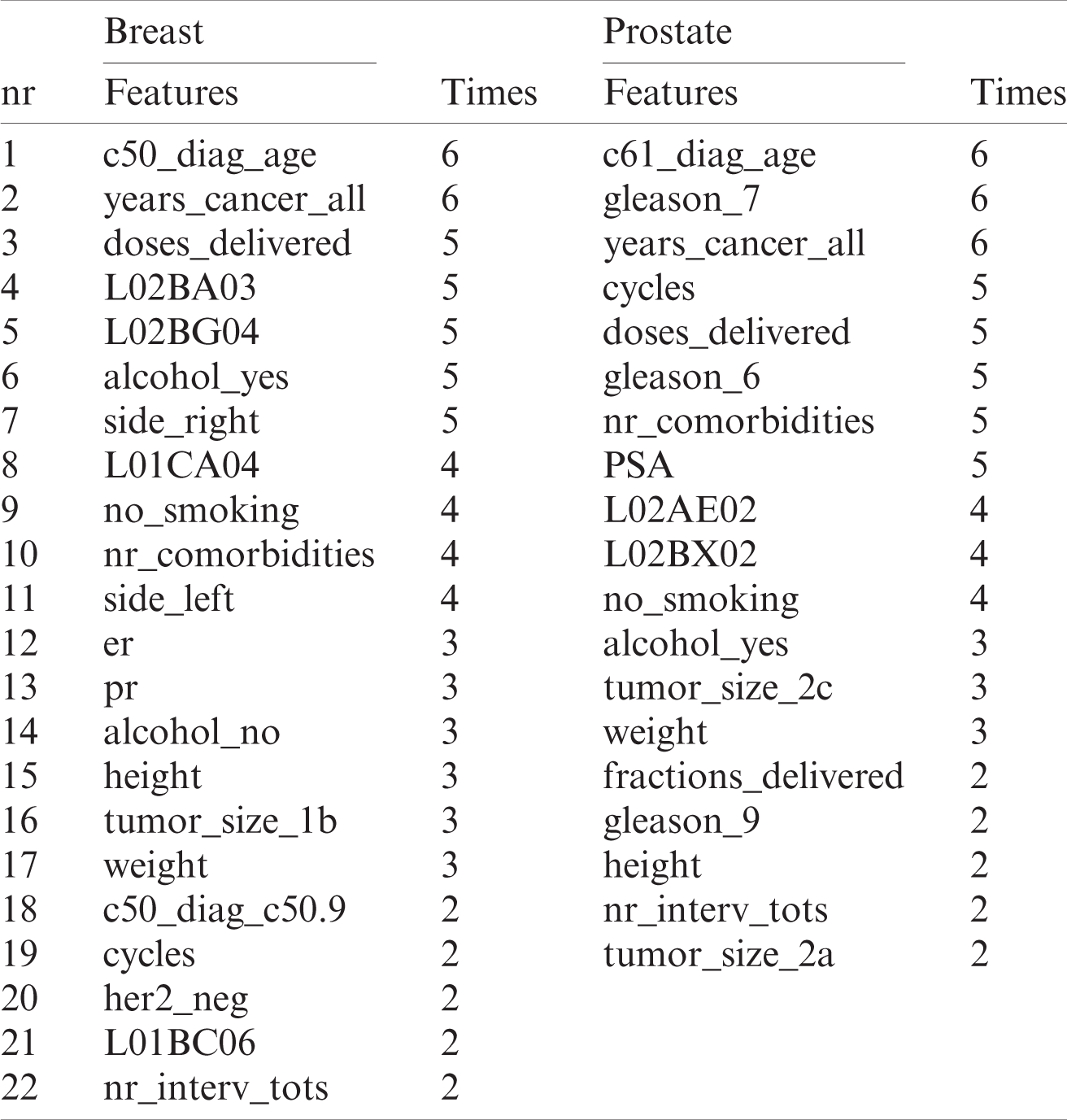
The final features selected for analysis are shown in Tab. 5. All the features are included that were chosen by at least two estimators, which is shown in the “times” (how many estimators chose the feature) columns for each cancer separately.
Table 5: Features selected for breast and prostate cancer data analysis
3.2 Classification Using Machine Learning
Nine different classification algorithms/estimators were selected for analysis, which was carried out after having chosen the features via the feature selection process. All estimators have several hyperparameters. A GridSearchCV was performed—an exhaustive search over specified parameter values for an estimator—to obtain the best hyperparameters for each algorithm. All parameters and values for each estimator are as follows.
1. LogisticRegression parameters:
2. ‘penalty’: [‘11,’ ‘l2,’ ‘elasticnet’],
3. ‘solver’: [‘lbfgs,’ ‘liblinear,’ ‘sag,’ ‘saga’],
‘max_iter’: [1000, 3000, 5000]
LinearSVC and SVC parameters:
a) ‘max_iter’: [1000, 3000, 5000],
b) ‘C’: [0.001, 0.01, 0.1]
SGDClassifier parameters:
a) ‘loss’: [‘hinge,’ ‘log,’ ‘squared_hinge,’ ‘perceptron’],
b) ‘alpha’: [0.0001, 0.001, 0.01, 0.1],
c) ‘penalty’: [‘l1,’ ‘l2,’ ‘elasticnet’]
KNeighborsClassifier parameters:
b) ‘algorithm’: [‘auto,’ ‘ball_tree,’ ‘kd_tree,’ ‘brute’]
BernoulliNB parameters:
a) ‘alpha’: [0.1, 0.2, 0.4, 0.6, 0.8, 1]
GaussianNB parameters: defaults
RandomForestClassifier and DecisionTreeClassifier parameters:
b) ‘min_samples_leaf’: [0.1, 0.12, 0.14, 0.16, 0.18]
The best value for each hyperparameter is displayed below in Tab. 6 for each estimator and disease:
Table 6: Selected best hyperparameters for each type of cancer

The Receiver Operating Characteristic (ROC) and AUC metric were used to assess classifier quality. The ROC curve features a true positive rate on the Y-axis and a false positive rate on the X-axis, meaning that the top left corner of the plot is the “ideal” point (a zero false positive rate and a one true positive rate) [41]. Although the “ideal point” is not realistic, it usually indicates that larger AUC is preferable. The ROC curve’s “steepness” is also essential since it is ideal for maximizing the true positive rate while minimizing the false positive rate.
Cross-validation was performed for each estimator using scikit-learn StratifiedKFold with the default value of the number of splits set to 5 (5-fold cross-validation). The ROC AUC curve for each estimator with cross-validation for breast cancer is shown in Fig. 2 and in Fig. 3 for prostate cancer.

Figure 3: ROC AUC for prostate cancer
It can be clearly seen that the support vector machine classifier achieved the best ROC AUC curve for the breast cancer dataset with an area under the
Conversely, the worst performances for the breast cancer dataset were identified by the following classifiers: Bernoulli Naïve Bayes with ROC
In addition, ensemble learning was performed using bagging and voting with cross-validation. BaggingClassifier was used for bagging, and VotingClassifier for voting. In the case of BaggingClassifier, the number of trees was set to 500, and KFold cross-validator was used for cross-validation. The ROC-AUC curve for the breast cancer dataset is shown in Fig. 4, and for the prostate cancer dataset in Fig. 5.
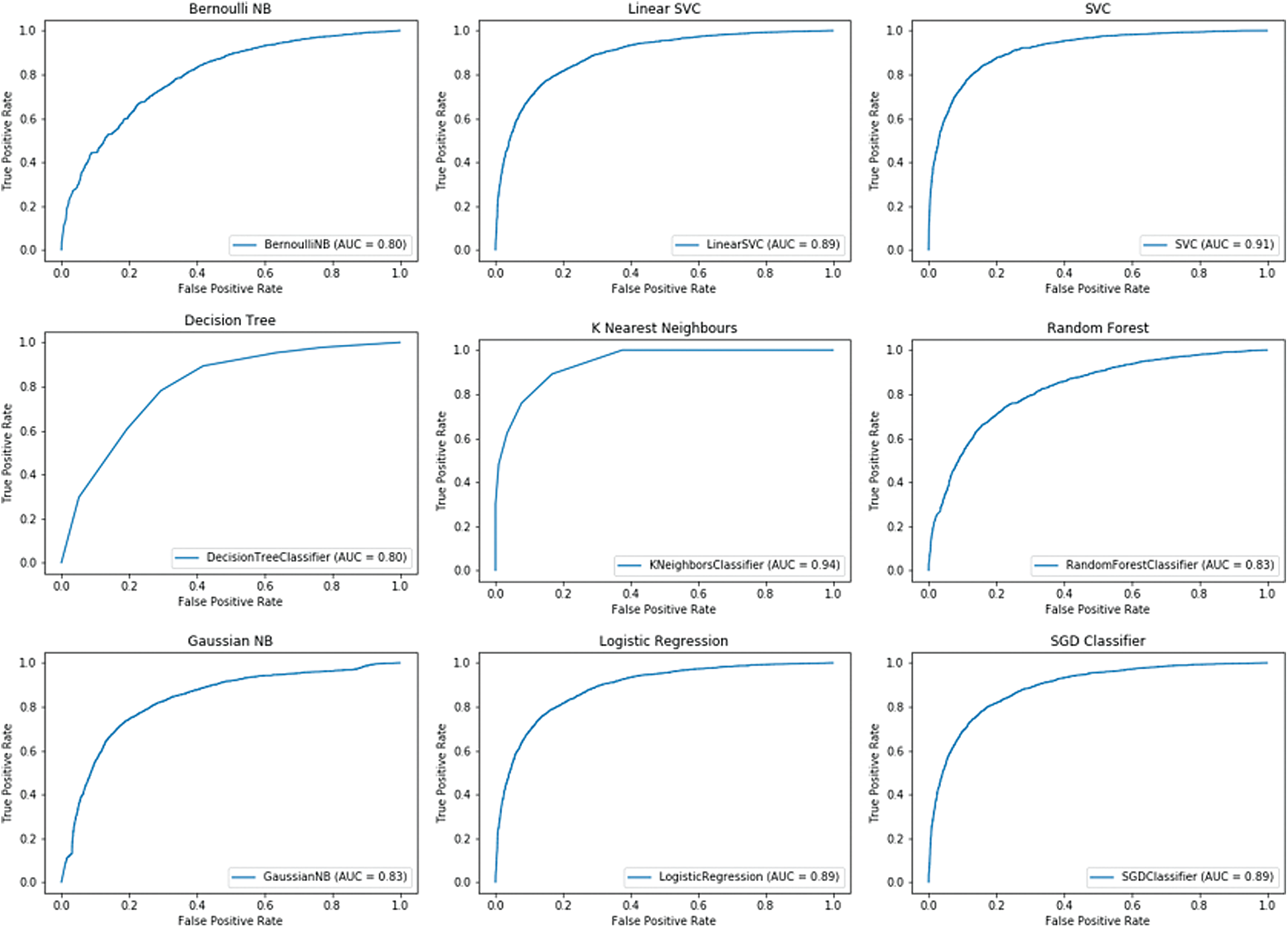
Figure 4: BaggingClassifier for breast cancer dataset

Figure 5: BaggingClassifier for prostate cancer dataset
As in the previous cross-validation analysis, the best results for BaggingClassifier, in the case of the breast cancer dataset, were yielded by KNeighborsClassifier with a ROC AUC
3.3 Comparing Machine Learning Models
The accuracy score, precision, recall and F1 score were selected in the training and test sets in order to compare how each model scored when predicting each patient’s survivability. Since the problem was a binary classification problem, the results for both classes are presented; the first class, class 0, being patients still alive, and the second, class 1, those who have died. Tab. 7 shows the results for the breast cancer dataset and Tab. 8 for the prostate cancer dataset. These results were obtained by using the classification_report imported from the sklearn library metrics module.
Table 7: Comparison of machine learning models results for breast cancer dataset

Table 8: Comparison of machine learning models results for prostate cancer dataset

In addition, the selected models were trained and tested using the voting technique, with and without data standardization. It was noted that when data standardization techniques were employed such as StandardScaler( ), better results were obtained on all counts for the BCa dataset. However, this was not the case for the PCa dataset. Recall in class 1 and precision in class 2 are slightly worse, but the others either remain unchanged, such as the accuracy scores and F1 score in class 1, or are marginally better.
In general, the algorithms performed better on the breast cancer dataset compared to prostate cancer. One reason could be dataset size; the BCa dataset is slightly larger and more balanced than the PCa dataset. Another reason could be the features. Despite using feature selection algorithms to select the most appropriate variables, other features that were omitted may improve the results.
There are multiple variables for each of these two types of cancer. This study sought to analyze which variables were of most importance when predicting patient survivability, or the mortality risk, within the first 15 years of cancer diagnosis. In total, 179 features were included on the breast cancer dataset and 144 on the prostate cancer dataset.
Valid results were obtained by only selecting 15 features after running different feature selection algorithms with different numbers of selected features. In other words, the difference in accuracy achieved by including all 179 features or just 15 features was insignificant.
The selected features are some of the main risk factors of these diseases. In both cancers, it is clear that age at diagnosis and years suffering from cancer are two of the main features that predict whether a patient will survive. Among the selected features, there are few relating to medications and lifestyle (see Tab. 9). Medications for BCa include L02BA03, L02BG04, L01CA04 and L01BC06; and L02AE02 and L02BX02 for PCa.
Table 9: Generic names and ATC codes for medication selected during the feature selection process

When attempting to predict the progression of these cancers, it is difficult to make comparisons between studies. This is due to the lack of large, publicly available datasets, numbers of records and number of variables the datasets contain. Moreover, there is a sheer number of hypotheses that these studies test. This can even be seen in the feature selection algorithms used by various authors. Earlier studies used the F-Score to reduce the number of variables [42,43], with more recent studies moving toward more sophisticated algorithms such as random forest [44,45] and genetic algorithms [46].
The database is very comprehensive and covers a wealth of data. This study has endeavored to include as much data as possible in its analytical approach. Nevertheless, laboratory results have not been included. The reason being that blood tests are routinely performed, and results vary depending on the treatment the patient is undergoing. Analyzing the averages of such results would fail to yield any meaningful results. However, other ways of incorporating this information into the analysis are being investigated. Another analysis method currently being developed is to conduct a similar study with different deep learning models and compare these results with the results obtained from the machine learning analysis.
Also, it should be noted that these results are specific to this Finnish population. Each country has its own guidelines and approved medications for certain diseases, so training the same models on a different dataset could deliver different results.
Acknowledgement: We wish to thank the Marie Sklodowska-Curie Action for funding the project and Success Clinic Oy for purchasing the dataset and welcoming O. B. to conduct her research.
Funding Statement: O. B. received funding from the European Union’s Horizon 2020 CATCH ITN project under the Marie Sklodowska-Curie grant agreement no. 722012, website https://www.catchitn.eu/.
Conflict of Interest: The authors declare that they have no conflicts of interest to report regarding the present study.
1. Cancer Society of Finland, “Facts about cancer,” 2020. [Online]. Available: www.allaboutcancer.fi [Accessed: 29 August 2020]. [Google Scholar]
2. Finnish Medical Society Duodecim and the Finnish Urological Association, “Prostate cancer,” Helsinki: The Finnish Medical Society Duodecim, 2014. [Online]. Available: https://www.kaypahoito.fi/en/about-current-care-guidelines/rights-of-use/quoting [Accessed: 02 August 2020]. [Google Scholar]
3. Finnish Cancer Registry, “Cancer statistics,” 2020. [Online]. Available: https://cancerregistry.fi/ [Accessed: 20 August 2020]. [Google Scholar]
4. S. Pakkanen, A. B. Baffoe-Bonnie, M. P. Matikainen, P. A. Koivisto, T. L. Tammela et al., “Segregation analysis of 1,546 prostate cancer families in Finland shows recessive inheritance,” Human Genetics, vol. 121, no. 2, pp. 257–267, 2007. [Google Scholar]
5. H. Grönberg, L. Damber and J. E. Damber, “Familial prostate cancer in Sweden: A nationwide register cohort study,” Cancer, vol. 77, no. 1, pp. 138–143, 1996. [Google Scholar]
6. O. Bratt, “Hereditary prostate cancer: Clinical aspects,” Journal of Urology, vol. 168, no. 3, pp. 906–913, 2002. [Google Scholar]
7. P. Lichtenstein, N. V. Holm, P. K. Verkasalo, A. Iliadou, J. Kaprioet et al., “Environmental and heritable factors in the causation of cancer—Analyses of cohorts of twins from Sweden, Denmark, and Finland,” New England Journal of Medicine, vol. 343, no. 2, pp. 78–85, 2000. [Google Scholar]
8. C. L. Van Patten, J. G. de Boer and E. S. Guns Tomlinson, “Diet and dietary supplement intervention trials for the prevention of prostate cancer recurrence: A review of the randomized controlled trial evidence,” Journal of Urology, vol. 180, no. 6, pp. 2312–2314, 2008. [Google Scholar]
9. S. Hori, E. Butler and J. McLoughlin, “Prostate cancer and diet: Food for thought?,” BJU International, vol. 107, no. 9, pp. 1348–1359, 2011. [Google Scholar]
10. Y. Liu, F. Hu, D. Li, F. Wang, L. Zhu et al., “Does physical activity reduce the risk of prostate cancer? A systematic review and meta-analysis,” European Urology, vol. 60, no. 5, pp. 1029–1044, 2011. [Google Scholar]
11. K. Zu and E. Giovannucci, “Smoking and aggressive prostate cancer: A review of the epidemiologic evidence,” Cancer Causes & Control, vol. 20, no. 10, pp. 1799–1810, 2009. [Google Scholar]
12. J. Mattsonand and L. Vehmanen, “Male breast cancer,” Duodecim, vol. 132, no. 7, pp. 627–631, 2016. [Google Scholar]
13. G. F. Stark, G. R. Hart, B. J. Nartowt and J. Deng, “Predicting breast cancer risk using personal health data and machine learning models,” Plos One, vol. 14, no. 12, pp. e0226765, 2019. [Google Scholar]
14. MDCalc, “Gail model for breast cancer risk,” 2021. [Online]. Available: https://www.mdcalc.com/gail-model-breast-cancer-risk [Accessed: 20 August 2020]. [Google Scholar]
15. I. Y. Gong, N. S. Fox, V. Huang and P. C. Boutros, “Prediction of early breast cancer patient survival using ensembles of hypoxia signatures,” Plos One, vol. 13, no. 9, pp. e0204123, 2018. [Google Scholar]
16. S. S. Thakur, H. Li, A. M. Y. Chan, R. Tudor, G. Bigras et al., “The use of automated Ki67 analysis to predict Oncotype DX risk-of-recurrence categories in early-stage breast cancer,” Plos One, vol. 13, no. 1, pp. e0188983, 2018. [Google Scholar]
17. N. Sapre, M. K. H. Hong, G. Macintyre, H. Lewis, A. Kowalczyk et al., “Curated microRNAs in urine and blood fail to validate as predictive biomarkers for high-risk prostate cancer,” Plos One, vol. 9, no. 4, pp. e91729, 2014. [Google Scholar]
18. D. P. Ankerst, G. Jack, R. Day John, B. Amy, R. Harry et al., “Predicting prostate cancer risk through incorporation of prostate cancer gene 3,” Journal of Urology, vol. 180, no. 4, pp. 1303–1308, 2008. [Google Scholar]
19. “Prostate Cancer Prevention Trial Risk Calculator,” 2018. [Online]. Available: http://riskcalc.org:3838/PCPTRC/ [Accessed: 20 August 2020]. [Google Scholar]
20. D. P. Ankerst, J. Straubinger, K. Selig, L. Guerrios, A. De Hoedt et al., “A contemporary prostate biopsy risk calculator based on multiple heterogeneous cohorts,” European Urology, vol. 74, no. 2, pp. 197–203, 2018. [Google Scholar]
21. S. M. Lynch, E. Handorf, K. A. Sorice, E. Blackman, L. Bealin et al., “The effect of neighborhood social environment on prostate cancer development in black and white men at high risk for prostate cancer,” Plos One, vol. 15, no. 8, pp. e0237332, 2020. [Google Scholar]
22. G. A. Stevens, L. Alkema, R. E. Black, J. T. Boerma, G. S. Collins et al., “Guidelines for accurate and transparent health estimates reporting: The GATHER statement,” PLoS Medicine, vol. 13, no. 6, pp. e1002056, 2016. [Google Scholar]
23. O. Bardhi and B. Garcia Zapirain, “The analysis of demographic, medical, and lifestyle data on treatment lines for breast and prostate cancer: Beacon Hospital case study,” International Journal of Environmental Research and Public Health, (under review2020. [Google Scholar]
24. World Health Organization, International Statistical Classification of Diseases and Related Health Problems, 10th Revision (ICD-10). Geneva: WHO, 1992. [Google Scholar]
25. F. Fioretti, A. Tavani, C. Bosetti, C. La Vecchia, E. Negri et al., “Risk factors for breast cancer in nulliparous women,” British Journal of Cancer, vol. 79, no. 11–12, pp. 1923–1928, 1999. [Google Scholar]
26. T. J. Pollard, A. E. W. Johnson, J. D. Raffa and R. G. Mark, “Tableone: An open source python package for producing summary statistics for research papers,” Jamia Open, vol. 1, no. 1, pp. 26–31, 2018. [Google Scholar]
27. G. Van Rossum and F. L. Drake, Python 3 Reference Manual. Scotts Valley, CA: CreateSpace, 2009. [Google Scholar]
28. L. Buitinck, G. Louppe, M. Blondel, F. Pedregosa, A. Mueller et al., “API design for machine learning software: experiences from the scikit-learn project,” in European Conf. on Machine Learning and Principles and Practices of Knowledge Discovery in Databases, Prague, Czech Republic, 2013. [Google Scholar]
29. A. C. Lorena, L. F. O. Jacintho, M. F. Siqueira, R. D. Giovanni, L. G. Lohmann et al., “Comparing machine learning classifiers in potential distribution modelling,” Expert Systems with Applications, vol. 38, no. 5, pp. 5268–5275, 2011. [Google Scholar]
30. J. V. Tu, “Advantages and disadvantages of using artificial neural networks versus logistic regression for predicting medical outcomes,” Journal of Clinical Epidemiology, vol. 49, no. 11, pp. 1225–1231, 1996. [Google Scholar]
31. C. Cortes and V. Vapnik, “Support-vector networks,” Machine Learning, vol. 20, no. 3, pp. 273–297, 1995. [Google Scholar]
32. O. Miguel-Hurtado, R. Guest, S. V. Stevenage, G. J. Neil and S. Black, “Comparing machine learning classifiers and linear/logistic regression to explore the relationship between hand dimensions and demographic characteristics,” PloS One, vol. 11, no. 11, pp. e0165521, 2016. [Google Scholar]
33. F. Pedregosa, G. E. Varoquaux, A. Gramfort, V. Michel, B. Thirion et al., “Scikit-learn: Machine learning in python,” Journal of Machine Learning Research, vol. 12, pp. 2825–2830, 2011. [Google Scholar]
34. T. Cover and P. Hart, “Nearest neighbor pattern classification,” IEEE Transactions on Information Theory, vol. 13, no. 1, pp. 21–27, 1967. [Google Scholar]
35. K. M. Al-Aidaroos, A. A. Bakar and Z. Othman, “Naïve Bayes variants in classification learning,” in Int. Conf. on Information Retrieval & Knowledge Management, pp. 276–281, 2010. [Google Scholar]
36. J. R. Quinlan, “Induction of decision trees,” Machine Learning, vol. 1, no. 1, pp. 81–106, 1986. [Google Scholar]
37. H. Saleh, “Chapter 1: Introduction to scikit-learn,” in Machine Learning Fundamentals: Use Python and Scikit-Learn to Get Up and Running with the Hottest Developments in Machine Learning. Birmingham, United Kingdom: Packt Publishing, pp. 1–37, 2018. [Google Scholar]
38. I. Guyon and A. Elisseeff, “An introduction to variable and feature selection,” Journal of Machine Learning Research, vol. 3, pp. 1157–1182, 2003. [Google Scholar]
39. T. Chen and C. Guestrin, “XGBoost,” in Proc. of the 22nd ACM SIGKDD Int. Conf. on Knowledge Discovery and Data Mining, pp. 785–794, 2016. [Google Scholar]
40. XGBoost developers, “XGBoost Python Package,” 2020. [Online]. Available: https://xgboost.readthedocs.io/en/latest/python/index.html [Accessed: 02 July 2020]. [Google Scholar]
41. T. Fawcett, “An introduction to ROC analysis,” Pattern Recognition Letters, vol. 27, no. 8, pp. 861–874, 2006. [Google Scholar]
42. M. F. Akay, “Support vector machines combined with feature selection for breast cancer diagnosis,” Expert Systems with Applications, vol. 36, no. 2, pp. 3240–3247, 2009. [Google Scholar]
43. C. Huang, H. Liao and M. Chen, “Prediction model building and feature selection with support vector machines in breast cancer diagnosis,” Expert Systems with Applications, vol. 34, no. 1, pp. 578–587, 2008. [Google Scholar]
44. C. Nguyen, Y. Wang and H. N. Nguyen, “Random forest classifier combined with feature selection for breast cancer diagnosis and prognostic,” Journal of Biomedical Science and Engineering, vol. 6, no. 5, pp. 551–560, 2013. [Google Scholar]
45. M. Huljanah, Z. Rustam, S. Utama and T. Siswantining, “Feature selection algorithm using random forest to diagnose cancer,” International Journal of Internet, Broadcasting and Communication, vol. 1, no. 1, pp. 10–15, 2009. [Google Scholar]
46. E. Aličković and A. Subasi, “Breast cancer diagnosis using GA feature selection and rotation forest,” Neural Computing and Applications, vol. 28, no. 4, pp. 753–763, 2015. [Google Scholar]
 | This work is licensed under a Creative Commons Attribution 4.0 International License, which permits unrestricted use, distribution, and reproduction in any medium, provided the original work is properly cited. |