Computers, Materials & Continua DOI:10.32604/cmc.2021.012095
Article

Modelling and Analysis of Bacteria Dependent Infectious Diseases with Variable Contact Rates

J. B. Shukla1, Shikha Singh2, Jitendra Singh2 and Sunil Kumar Sharma3,*

1Innovative Internet University for Research, Kanpur, 208017, India
2P.P.N.(P.G.) College, CSJM University, Kanpur, 208001, India
3College of Computer and Information Sciences, Majmaah University, Majmaah, 11952, Saudi Arabia
*Corresponding Author: Sunil Kumar Sharma. Email: s.sharma@mu.edu.sa
Received: 20 June 2020; Accepted: 30 August 2020

Abstract: In this research, we proposed a non-linear SIS model to study the effect of variable interaction rates and non-emigrating population of the human habitat on the spread of bacteria-infected diseases. It assumed that the growth of bacteria is logistic with an intrinsic growth rate is a linear function of infectives. In this model, we assume that contact rates between susceptibles and infectives as well as between susceptibles and bacteria depend on the density of the non-emigrating population and the total population of the habitat. The stability theory has been analyzed to analyzed to study the crucial role played by bacteria in the increased spread of an infectious disease. It is shown that as the density of non-emigrating population increases, the spread of an infectious disease increases. It is shown further that as the emigration increases, the spread of the disease decreases in both the cases of contact mentioned above rates, but this spread increases as these contact rates increase. It suggested that the control of bacteria in the human habitat is very useful to decrease the spread of an infectious disease. These results are confirmed by numerical simulation.

Keywords: Mathematical modelling; density dependent contact rates; stability analysis

1  Introduction

Most of the deaths worldwide are caused due to infectious diseases. A severe threat to the wellbeing and public health is caused not only due to the new infectious diseases but also due to the increasing prevalence of drug-related diseases as well as the resurgence of chronic infectious diseases. Recently, considerable evidence found to suggest that common strategies are adopted by different pathogens to cause disease and infection. The infectious organism causes Infectious diseases; these are bacteria, viruses, fungi, etc. Under normal circumstances, disease symptoms may not develop when the immune system of the host is fully functional, but an infectious disease ensues if the immune system of the host is compromised. Bacteria, protozoa, viruses, etc. cause most of the infections in living organisms. Bacteria is a unicellular prokaryotic micro-organism. In the human habitat, due to household emission, various kinds of carriers and vectors grow and survive. They become agents to carry bacteria to food and water of Susceptibles, causing them to be infected by various diseases. Notably, in habitats, which are not clean enough, various types of bacteria such as mycobacterium tuberculosis, vibrio cholera etc. are present, the growth rate of which depends upon the following factors:

•    The Bacteria discharges by infective in the environment.

•    The characteristics of household discharges such as nutrients, salts, amino acids, and vitamins etc.

•    The characteristics of bacteria related to particular diseases such as TB, Typhoid etc.

•    The natural conditions such as the climate of the habitat.

Therefore, we assume that the bacteria population density is proportional to the density of carriers, such as house flies, and hence its growth rate is assumed to follow the logistic model [1]. These bacteria get transported by carriers to susceptible and their food as well as water, making them infectives indirectly [2]. Mathematical models have been used in the study of the spread and control of infectious diseases for a long time. In classical models, the contact rates between susceptible and infectives have been assumed to be constant [3–6], but recently the effect of density-dependent contact rate, death rate etc. on the spread of infectious diseases have been studied. However, the effect of the non-emigrating population of the habitat on the spread of the infectious disease has never been considered in various studies. However, in a realistic situation, the contact rates between susceptible and infectives as well as between susceptible and bacteria depends upon the density of non-emigrating population [7–9]. The massive consumption of alcohol affects almost all parts of the body, which in turn responsible for gonorrhea, which is a bacterial disease. This disease infects the parts of the body like urine, eyes, throat, vagina anus, and the female’s fallopian tubes, uterus etc. [10]. Recently researchers work in the field of application of mathematical modeling multiscale fast correlation filtering tracking algorithm [11], grammar model [12], grammar mapping and the integer modulo Arithmetic [13] and decision model of knowledge [14] transfer The spread of an infectious disease can be controlled by using awareness programs. However, the disease remains endemic due to immigration [11,12,15,16].

Therefore, we proposed a non-linear mathematical model to study the effects of the following aspects of the spread of bacteria-infected diseases:

•    Effect of the non-emigrating population of the habitat.

•    Effect of emigration dependent contact rate between susceptible and infective population as well as between susceptible and bacteria population.

•    Effects of discharge of bacteria by infectives in the habitat.

•    Effect of control of bacteria by using chemicals and pesticides.

2  Mathematical Model with Emigration Dependent Contact Rates

Let the total human population of the habitat at time t be N(t), which consists of the susceptible population density X(t) and infective population density Y(t). We assume that the susceptible population of the habitat may be affected by the bacterial populations with density B(t) (Fig. 1). The bacteria population grows logistically with its intrinsic growth rate coefficient as a linear function of infective population Y(t). The contact rate β(N) between susceptibles and infectives is assumed to be emigration dependent, and the contact rate λ(N) between susceptibles and bacteria depends upon the densities of non-emigrating population and the total population N. It is assumed as follows,

β(N)=β-β0(N-N0),(1)

where, N0 is the non-emigrating population density of the habitat which is a fraction of N, β and β0 are constant contact rate coefficients. It is noted from Eq. (1), β(N) increases as N0 increases, but it decreases as β0 increases.

Figure 1: Interaction phenomena between susceptibles and infectives

Similarly, the emigration dependent contact between susceptibles and bacteria population is assumed to be a non-negative linear function of the total population as,

λ(N)=λ-λ0(N-N0),(2)

where, λ and λ0 denotes the contact rate coefficients. From Eq. (2) as N0 increases, λ(N) increases but λ(N) decreases as λ0 increases. The primary purpose of this paper is to study the effect of variable contact rate between susceptibles and infectives, variable contact rate between susceptibles and bacteria, and non-emigrating population on the spread of bacteria-infected disease and the growth of bacteria due to infectives.

In view of the above situation, the diseases dynamics model given below:

dXdt=A-{β-β0(N-N0)}XY-{λ-λ0(N-N0)}XB-dX+νYdYdt={β-β0(N-N0)}XY+{λ-λ0(N-N0)}XB-(ν+α+d)YdBdt=(θ+ϕY)B-θ0B2-ϕ0B,(3)

where, X(0) = X0 > 0, Y(0)=Y0≥0,N(0)=N0>0,B(0)=B0≥0 and N = X + Y.

The model system Eq. (3) has the following parameters:

•    A: Immigration rate of the human population from outside.

•    β: Interaction coefficient due to infective human population density.

•    β0: Emigration dependent transmission coefficient due to infectives density.

•    λ: Constant transmission coefficient due to bacteria population density.

•    λ0: Emigration dependent transmission coefficient due to bacteria population density.

•    d: Natural death rate coefficient.

•    α: Disease related death rate coefficient.

•    ν: Recovery rate coefficient.

•    θ: Growth rate coefficient of bacteria population due to natural conducive factors in the habitat.

•    θ0: Natural depletion rate coefficient of bacteria population.

•    ϕ: Growth rate coefficient of bacteria by the discharge of the infective population.

•    ϕ0: The control rate of bacteria population by using chemicals and pesticides etc.

The model system Eq. (3) is reduced as follows by using X = N − Y and θs=θ-ϕ0>0, we get

dYdt={β-β0(N-N0)}(NY-Y2)+{λ-λ0(N-N0)}(N-Y)B-(d+ν+α)Y (4)

dNdt=A-αY-dN (5)

dBdt=(θs+ϕY)B-θ0B2 (6)

With the initial conditions: Y(0)=Y0≥0, N(0) = N0 > 0, B(0)=B0≥0.

Region of attraction: The following set gives the domain region of the model system Eqs. (4)–(6) as

Ω={(Y,N,B)∈R+3:0≤Y≤A(α+d),A(α+d)≤N≤Ad,0≤B≤Bm}.(7)

where, Bm=θsθ0+ϕAθ0(α+d).

3  Basic Reproduction Number and Equilibrium Analysis of the Model

The basic reproduction number R0 is used to measure the transmission potential of a disease. It is the average number of secondary infections produced by an infection in a human habitat where the living population is susceptible [17,18].

The non-linear mathematical model Eqs. (4)–(6) has three non-negative equilibria as:

1. E0(0,Ad,0), this is the trivial equilibrium point which exists always.

2. E1(Y¯,N¯,0), this is the bacteria-free equilibrium point, which exists if the reproduction number

R0=(β+β0N0)Ad(ν+α+d)+β0A2d2>1.(8)

3. E2(Y*,N*,B*), this is the non-trivial equilibrium point, which exists if

R1={(β+β0N0)+(λ+λ0N0)ϕθ0+λ0θs(d+2α)θ0d}Ad(ν+α+d)+(λ+λ0N0)θs(α+d)θ0d+(β0+λ0ϕθ0)A2d2>1.(9)

It is noted that when λ=0, λ0=0 then R1 = R0.

Proof. The equilibrium point E0 exists obviously. For the model system Eqs. (4)–(6), we prove the existence of E1(Y¯,N¯,0). Let Y≠0 and B = 0 then Y¯ and N¯ are the solution, which is obtained from the following two equations:

{β-β0(N-N0)}(N-Y)-(ν+α+d)=0. (10)

A-dN-αY=0. (11)

By using Eqs. (10) and (11) we define a polynomial function in Y as,

F(Y)={(β+β0N0-β0Ad)Ad-(ν+α+d)}+{β0αAd2-(α+d)d(β+β0N0-β0Ad)}Y-{α(α+d)d2β0}Y2=0(12)

We note from Eq. (12),

•    F(0)={(β+β0N0-β0Ad)Ad-(d+ν+α)}>0 for R0 > 1.

•    F(Aα+d)=-(ν+α+d)<0.

Thus, the equation F(Y) = 0 has at least one root Y∈(0,Aα+d). To show the root is unique, we show that F′(Y) < 0. By differentiating Eq. (12) with respect to Y, we get

F′(Y)=0+{β0αAd2-(α+d)d(β+β0N0-β0Ad)}-{α(α+d)d2β0}2Y(13)

then, by using Eq. (12) in Eq. (13), we get

YF′(Y)=-{(β+β0N0-β0Ad)Ad-(ν+α+d)}-{α(α+d)d2β0}Y2<0(14)

Hence F′(Y) < 0 for R0 > 1. Thus a unique root of F(Y) = 0, Y¯ exists. Now by using the value of Y¯, the value of N¯ can be uniquely determined from Eq. (11).

The other equilibrium point E2(Y*,N*,B*) is obtained by solving the following equations:

(β-β0(N-N0))(N-Y)Y+(λ-λ0(N-N0))(N-Y)B-(d+ν+α)Y=0. (15)

A-αY-dN=0. (16)

θs-θ0B+ϕY=0. (17)

By using the equations Eqs. (16) and (17) in Eq. (15) and setting

βm=β+β0N0-β0Ad,λm=λ+λ0N0-λ0Ad and θs=θ-ϕ0.

We define the following function

H(Y)={λmAθsθ0d}+{βmAd-(ν+α+d)+λmAϕθ0d-λm(α+d)θsθ0d+λ0Aαθsd2θ0}Y+{β0Aαd2-βm(α+d)d-λmϕ(α+d)θ0+d+λ0ϕAαθ0d2-λ0α(α+d)θsθ0d2}Y2-{β0α(α+d)d2+λ0αϕ(α+d)θ0d2}Y3.(18)

It is noted from Eq. (18)

•    H(0)=λmAθsθ0d>0.

•    H(A(α+d))=-(ν+α+d)A(α+d)<0.

Hence, the equation H(Y) = 0 has at least one root in Y∈(0,Aα+d). To show the uniqueness of root Y∈(0,Aα+d), We need to show that H′(Y) < 0. For this, we differentiate Eq. (18) with respect to Y, we get

H′(Y)=0+{ βmAd−(ν+α+d)+λmAϕθ0d−λm(α+d)θs)dθ0+λ0Aαθsθ0d2 }  { β0Aαd2−βm(α+d)d−λmϕ(α+d)θ0+d+λ0ϕAαθ0d2−λ0α(α+d)θsθ0d2 }2Y −{ β0α(α+d)d2+λ0αϕ(α+d)θ0d2 }3Y2(19)

By using Eq. (18) in Eq. (19), we have

YH′(Y)=−2λmAθsθ0d−{ βmAd−(ν+α+d)+λmAϕθ0d−λm(α+d)θs)θ0d +λ0Aαθsθ0d2 }Y−{ β0α(α+d)d2+λ0αϕ(α+d)θ0d2 }Y3<0.(20)

Provided R1 > 1, where R1 is the reproduction number. Hence the equation Eq. (18) have unique root in the interval Y∈(0,Aα+d).

4  Stability Analysis

The stability of the equilibrium points E0(0,Ad,0), E1(Y¯,N¯,0) and E2(Y*,N*,B*) are stated in the following two theorems [19]. The equilibrium points E0(0,Ad,0) and E1(Y¯,N¯,0) are unstable and E2(Y*,N*,B*) is locally asymptotically stable provided the following conditions are satisfied

α{(β0Y*+λ0B*)(N*-Y*)}2<d{β(N*)Y*+B*λ(N*)}2. (21)

2ϕ2{(N*-Y*)λ(N*)}2<θ02{β(N*)Y*+B*λ(N*)}2. (22)

Proof. See Appendix A.

The equilibrium point E2(Y*,N*,B*) is non-linearly stable in Ω provided the following conditions are satisfied:

α{(β0Y*+λ0Bm)Ad}2<d{Y*β(N*)+B*λ(N*)}2. (23)

2ϕ2{λ(N*)Ad}2<θ02{β(N*)Y*+B*λ(N*)}2. (24)

where, Bm is defined in Section 2 Eq. (7).

Proof. See Appendix B: It is noted from Eq. (4), the inequalities Eqs. (23) and (24) are stronger than inequalities Eqs. (21) and (22), as expected. Further, the inequalities Eqs. (21) and (23) are satisfied automatically when α=0. Also, when ϕ=0, then inequalities Eqs. (22) and (24) are satisfied automatically. Hence the death rate related coefficient and rates of growth of bacteria caused by infective population density have destabilizing effects on the system.

5  Numerical Simulation of the Model

By using MAPLE, we show the existence and stability of the equilibrium point E2(Y*,N*,B*) for the following set parameters as given in Tab. 1 value of the set of parameters

Table 1: Value of parameters

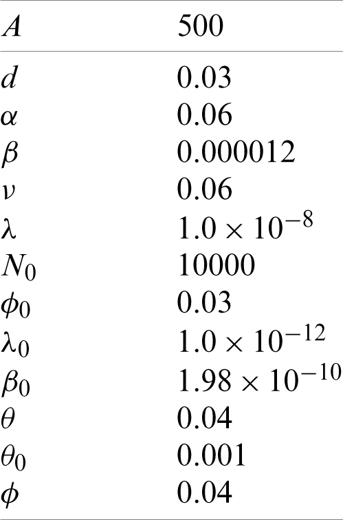
For these values of parameters, the value of the non-trivial equilibrium point E2(Y*,N*,B*) corresponding to Eqs. (4)–(6) is obtained as follows:

Y*=1155.45≈1155,N*=14355.75≈14356,B*=46228.23≈46228

The Jacobian matrix at E2(Y*,N*,B*) is

[-0.01611075840.0094996899460.00007450572410-0.06-0.0301849.1295890-46.22823972]

The eigenvalues of the above matrix at E2(Y*,N*,B*) are:

-0.02156484178+0.02233366797i,-0.02156484178-0.02233366797i,-46.23122079.

Since the sign of one eigenvalue is negative and two of them having negative real part, therefore the non-trivial equilibrium point E2(Y*,N*,B*) is stable asymptotically. It is noted here that for the assumed set of positive parameters, the conditions Eqs. (21)–(24) are satisfied. By using MAPLE software, the graph of Y vs. N for the model Eqs. (4)–(6) is shown in Fig. 2, which indicated the non-linear stability of the equilibrium point in the YN plane.

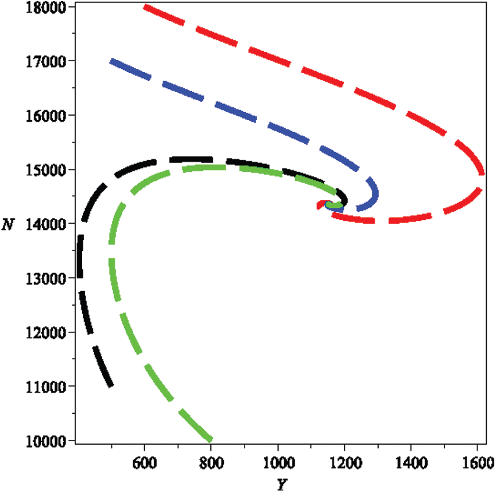
Figure 2: Phase plots between infected human population density Y(t) and human population density N(t)

It depicted in Fig. 3, as β increases, the number of infectives increases. From Fig. 4, we can see that as the emigration dependent contact rate β0 between susceptibles and infectives increases, the number of infectives decreases. From Fig. 5, as constant contact rate λ between susceptible and bacterial population increases, the number of infectives increases and from Fig. 6, as emigration dependent contact rate λ0 between susceptibles and Bacteria population density of habitat increases, then the number of infectives decreases. From Fig. 7, it is also observed that as the growth rate coefficient of bacteria due to infective population increases, the infectives increases. It observed from Fig. 8, that as the constant depletion rate coefficient ϕ0 increases, the spread of the disease decreases, and from Fig. 9, as the natural growth rate θ of bacteria increases, the spread of bacteria-infected disease increases. From Fig. 10, we observed that immigration increases, then the number of infectives increases, and from Fig. 11, as non-emigrating population increases, then the number of infective populations increases.

Figure 3: Effect of transmission coefficient β due to infectives on infective population density Y

Figure 4: Effect of emigration coefficient β0 due to infectives on infective population density Y

Figure 5: Effect of transmission coefficient λ due to bacteria population density on infective population density Y

Figure 6: Effect of emigration coefficient λ0 due to bacteria population density on infective population density Y

Figure 7: Effect of growth rate coefficient ϕ of bacteria due to infective population density on infective population density Y

Figure 8: Effect of the depletion rate coefficient ϕ0 of bacteria due to chemicals and pesticides etc. on infective population density Y

Figure 9: Effect of the natural growth rate coefficient of bacteria population θ on infective population density Y

Figure 10: Effect of constant immigration rate A on infective population density Y

Figure 11: Effect of non-emigrating population N0 on infective population density Y

6  Conclusions

In this study, an SIS non-linear model with emigration has been proposed and analyzed to study the effects of the following factors on the spread of bacteria-infected diseases.

•    Effect of non-emigrating population.

•    Effect of the emigration dependent contact rate between susceptibles and infectives, which is dependent on non-emigrating population and the total human population in the habitat.

•    Effect of the emigration dependent contact rate between susceptibles and bacteria population, which depends on non-emigrating population and the total population in the habitat.

•    Effect of the discharge rate of bacteria by the infectives in the habitat.

•    Effect of the growth rate of bacteria, which is assumed to follow the logistic model, the growth rate of which is a linear function of the infective population.

Using the stability theory, the analysis of the model has shown the following results.

•    As the discharge rate of bacteria by infectives increases, the spread of bacteria-infected disease increases.

•    As the non-emigrating population density increases, the spread of bacteria-infected diseases increases.

•    As the direct contact rate between susceptibles and infectives increases, the spread of a bacteria infected disease increases.

•    As the contact rate between susceptibles and bacteria population increases, the spread of bacteria infected disease increases.

•    As the emigration rate increases, the spread of bacteria-infected disease decreases.

•    As the natural growth rate of bacteria increases, the spread of an infectious disease increases.

•    As the immigration rate increases, the spread of bacteria-infected disease increases.

•    As the control rate of bacteria in the habitat increases, the spread of the disease decreases.

The simulation study of the non-linear model confirms the above outcomes. It has been concluded that if the bacteria population in the habitat controlled by using pesticides, the spread of bacteria-infected disease can be reduced considerably.

Acknowledgement: The authors would like to express their heartfelt thanks to the editors and anonymous referees for their most valuable comments and constructive suggestions which leads to the significant improvement of the earlier version of the manuscript. The authors are thankful to the Deanship of Scientific Research at Majmaah University.

Funding Statement: Dr. Sunil Kumar Sharma would like to thank Deanship of Scientific Research at Majmaah University for supporting this work under the Project No. R-2021-8.

Conflicts of Interest: The authors declare that they have no conflicts of interest to report regarding the present study.

Appendix A. Proof of Theorem 4.1

Proof. The model system Eqs. (4)–(6) as:

dYdt={β-β0(N-N0)}(NY-Y2)+{λ-λ0(N-N0)}(NB-YB)-(d+ν+α)Y (25)

dNdt=A-αY-dN (26)

dBdt=(θs+ϕY)B-θ0B2 (27)

For the above model system Eqs. (4)–(6), the Jacobian matrix is defined for the system as [A11A12(N-Y)λ(N)-α-d0ϕB0θs-θ0B+ϕY] where, A11=β(N)(N-2Y)-λ(N)B-(ν+α+d) and A12=β(N)Y-(β0+λ0)(YN-Y2)+λ(N)B.

The Jacobian matrix for the first equilibrium point E0(0,Ad,0) is

[β(Ad)Ad-(d+ν+α)0λ(Ad)Ad-α-d000θs]

From the above Jacobian matrix, it is clear that one of the eigenvalues is θs>0. Hence the disease and the bacteria-free equilibrium point E0(0,Ad,0) is unstable. Now the Jacobian matrix for the second equilibrium point E1(Y¯,N¯,0) is

[β(N¯)(N¯-2Y¯)-(ν+d+α)β(N¯)Y¯-β0(Y¯N¯-Y¯2)λ(N¯)(N¯-Y¯)-α-d000θs+ϕY¯]

It is clear from the above Jacobian matrix, one eigenvalue θs+ϕY¯ is positive. Hence the bacteria-free equilibrium point E1(Y¯,N¯,0) is unstable. We study the local stability behavior of E2(Y*,N*,B*) by direct Lyapunov’s method. Here we use the transformation of variables to linearize the model system as

Y-Y*=y,N-N*=n,B-B*=b and by considering a positive definite function V as:

V=12y2+k12n2+k22b2(28)

Differentiating Eq. (27) with respect to t, we get

V̇=yẏ+k1nṅ+k2bḃ(29)

The linearization of the functions gives,

ẏ={-(Y*β(N*)+λ(N*)B*)-λ(N*)(N*-Y*)B*Y*}y+{β(N*)Y*+λ(N*)B*-(N*-Y*)(β0Y*+λ0B*)}n+{(N*-Y*)λ(N*)}bṅ=-αy-dnḃ=ϕB*y-θ0B*b (32)

Then by Eq. (28), we have

V̇=-{β(N*)Y*+λ(N*)B*+(N*-Y*)λ(N*)B*Y*}y2+{β(N*)Y*+λ(N*)B*-(N*-Y*)×(β0Y*+λ0B*)}ny+{(N*-Y*)λ(N*)}by-k1dn2-k1αny+k2ϕB*by-k2θ0B*b2(33)

Here we choose the constant k1 such that k1=Y*β(N*)+B*λ(N*)α, we get

V̇={-(N*-Y*)B*λ(N*)Y*}y2+[-14{Y*β(N*)+λ(N*)B*}y2-{(β0Y*+λ0B*)(N*-Y*)}ny-k1dn2]+{-12{Y*β(N*)+λ(N*)B*}y2+λ(N*)(N*-Y*)by-12k2θ0B*b2}+{-14{Y*β(N*)+λ(N*)B*}y2+k2ϕB*by-12k2θ0B*b2}(34)

The derivative V̇<0 if the following inequalities hold.

{(β0Y*+λ0B*)(N*-Y*)}2<{Y*β(N*)+B*λ(N*)}k1d (35)

{(N*-Y*)λ(N*)}2<{Y*β(N*)+B*λ(N*)}k2θ0B* (36)

2{ (k2ϕB∗ }2<{ Y∗β(N∗)+B∗λ(N∗) }k2θ0B∗ (37)

By combining conditions Eqs. (35), (36) and on substituting the value of k1 in Eq. (34), we get the conditions as stated in Theorem 4.

α{(N*-Y*)(β0Y*+λ0B*)}2<d{β(N*)Y*+B*λ(N*)}2 (38)

2ϕ2{(N*-Y*)λ(N*)}2<θ02{β(N*)Y*+B*λ(N*)}2 (39)

Appendix B. Proof of Theorem 4.2

Proof. We consider the Lyapunov function,

U={(Y-Y*)-Y*(lnY-lnY*)}+K12(N-N*)2+K2{(B-B*)-B*(lnB-lnB*)}(40)

On differentiating Eq. (39) with respect to ‘t’, we get

U̇=ẎY(Y-Y*)+K1Ṅ(N-N*)+K2(B-B*)ḂBU̇={-(N-Y)Bλ(N)YY*(Y-Y*)2-(β(N*)+λ(N*)B*Y*)(N-N*)(Y-Y*) (41)

-(β0+λ0BY*)(N-Y)(N-N*)(Y-Y*)+λ(N*)(N-Y)Y*(Y-Y*)(B-B*)} (42)

By choosing K1=β(N*)Y*+λ(N*)B*αY*, we can write the equation Eq. (41) as:

U̇=-{(N-Y)Bλ(N)YY*}(Y-Y*)2+{-14(β(N*)+B*Y*λ(N*))(Y-Y*)2-(β0+λ0BY*)(Y-N)(Y-Y*)(N-N*)-K1d(N-N*)2}+{-12(β(N*)+B*Y*λ(N*))(Y-Y*)2+λ(N*)(N-Y)Y*(Y-Y*)(B-B*)-12K2θ0(B-B*)2}+{-14(β(N*)+B*Y*λ(N*))(Y-Y*)2+K2ϕ(B-B*)(Y-Y*)-12K2θ0(B-B*)2}(43)

For U̇<0, the following inequalities must satisfy for all values of parameters.

{(β0+λ0BY*)(N-Y)}2<{β(N*)+B*Y*λ(N*)}K1d (44)

α{(β0Y*+λ0Bm)Ad}2<d{β(N*)Y*+λ(N*)B*}2 (45)

and,

{(N-Y)λ(N*)Y*}2<{β(N*)+B*Y*λ(N*)}K2θ0 (46)

2{K2ϕ}2<{β(N*)+B*Y*λ(N*)}K2θ0 (47)

By combining the inequalities Eqs. (45)–(46)

2ϕ2{(N-Y)λ(N*)}2<θ02{β(N*)Y*+λ(N*)B*}2 (48)

2ϕ2{ Adλ(N∗)) }2<θ02{ β(N∗)Y∗+B∗λ(N∗) }2 (49)

Hence the non-trivial equilibrium point is non-linearly stable in Ω provided the following inequalities holds.

α{(β0Y*+λ0Bm)Ad}2<d{Y*β(N*)+B*λ(N*)}2 (50)

2ϕ2{ Adλ(N∗)) }2<θ02{ β(N∗)Y∗+B∗λ(N∗) }2 (51)

This work is licensed under a Creative Commons Attribution 4.0 International License, which permits unrestricted use, distribution, and reproduction in any medium, provided the original work is properly cited.