Computers, Materials & Continua DOI:10.32604/cmc.2021.016829
Article

Deep Reinforcement Learning for Multi-Phase Microstructure Design

Jiongzhi Yang, Srivatsa Harish, Candy Li, Hengduo Zhao, Brittney Antous and Pinar Acar*

Virginia Polytechnic Institute and State University, Blacksburg, 24061, VA, USA
*Corresponding Author: Pinar Acar. Email: pacar@vt.edu
Received: 12 January 2021; Accepted: 13 February 2021

Abstract: This paper presents a de-novo computational design method driven by deep reinforcement learning to achieve reliable predictions and optimum properties for periodic microstructures. With recent developments in 3-D printing, microstructures can have complex geometries and material phases fabricated to achieve targeted mechanical performance. These material property enhancements are promising in improving the mechanical, thermal, and dynamic performance in multiple engineering systems, ranging from energy harvesting applications to spacecraft components. The study investigates a novel and efficient computational framework that integrates deep reinforcement learning algorithms into finite element-based material simulations to quantitatively model and design 3-D printed periodic microstructures. These algorithms focus on improving the mechanical and thermal performance of engineering components by optimizing a microstructural architecture to meet different design requirements. Additionally, the machine learning solutions demonstrated equivalent results to the physics-based simulations while significantly improving the computational time efficiency. The outcomes of the project show promise to the automation of the design and manufacturing of microstructures to enable their fabrication in large quantities with the utilization of the 3-D printing technology.

Keywords: Deep learning; reinforcement learning; microstructure design

1  Introduction

Advancements in 3-D printing technology enabled the automation of the design and manufacturing of high-performance engineering materials. For example, computational models and machine learning (ML) techniques have an increasingly critical role in the design of 3-D printed microstructures as testing all possible microstructural combinations with a purely experimental approach remains infeasible. Accordingly, the present work focuses on the development and integration of ML methods into a physics-based simulation environment to enable and accelerate the design of 3-D printed multi-phase microstructures for different engineering applications. The current 3-D printing technology can produce structures that are made of multiple phases by utilizing different base materials. The multi-phase structures can provide complementary properties by balancing the desired features of the base materials. Our goal in this study is to find the optimum material properties of 3-D printed microstructures to improve the performance of engineering components under mechanical and thermo-mechanical loads and dynamic effects. The design optimization is first performed using a finite element model. Although finite element methods produce high-fidelity solutions, the computation times required for design studies may be excessive. Therefore, this study investigates the compatibility of ML and design optimization to produce computationally efficient results while maintaining a high level of accuracy.

The ML paradigm has attracted a lot of interest from materials modeling and design communities [1–7] as it enables the integration of mathematical techniques/data science tools into experiments and/or physical models. ML has been recognized as a complementary and powerful tool to accelerate the design and discovery of new-generation materials [8,9]. Prominent applications in this field include the design of 3-D printed composites involving multiple phases to improve the mechanical performance of materials [10–12] and ML-driven crystal plasticity modeling and design of polycrystalline microstructures [13–16]. Although these previous studies focused on more rigorous mechanical problems in terms of the number of design variables and complexity of the objectives, the goal of the present work is to implement different mathematical strategies for the ML-driven design of 3-D printed multi-phase microstructures. Accordingly, different ML-driven design strategies are presented in this study by utilizing Q-Value Reinforcement Learning (RL), Deep RL, and feed-forward artificial neural networks (ANN). The design optimization strategy with the integration of the ML solutions demonstrates a promising methodology that can be adapted in the future to more complicated design problems for multi-phase materials. The organization of the paper is described next. Section 2 discusses the finite element-based design of multi-phase microstructures. Section 3 presents the ML techniques and the results obtained with ML-driven solutions. A summary of the study with potential future extensions is provided in Section 4.

2  Finite Element Modeling

3-D printed multi-phase microstructures are assumed to demonstrate orthotropic material properties. Due to the directional independent nature of orthotropic properties, there are 9 independent variables that make up the compliance matrix in the global frame. For assembly and solution purposes, the inverse of the compliance matrix is used to construct the stiffness matrix which will be used in the local and global finite element system. The stress--strain equation for a three-dimensional orthotropic material is given as follows:

{σxxσyyσzzσzxσyzτxy}=⌈C11C12C13000C12C22C23000C13C23C33000000C44000000C55000000C66⌉{ϵxxϵyyϵzzγzxγyzγxy} (1)

where the stiffness coefficients (Cij values) are calculated from the orthotropic material properties (Young’s modulus values: Exx, Eyy; Poisson’s ratios: νxy, νyz and shear modulus: Gxy, Gyz). This relationship is then used to solve an orthotropic plate problem that describes a periodic multi-phase microstructure. Carbon Epoxy and Boron Epoxy are used as base materials of the microstructure; therefore, the design is expected to demonstrate properties that range within the property values of the base materials. Carbon Epoxy and Boron Epoxy material properties can be found in Reference [17] and shown in Tab. 1. The microstructure is assumed to demonstrate geometric periodicity, as visualized in Fig. 1. The plate problem is broken up into 2151 quadrilateral finite elements. The von Mises stress (VMS), which is traditionally used to predict yielding, is utilized as the stress measure. Three different design problems are considered to optimize the performance of the periodic microstructure: (i) Minimization of the maximum VMS value throughout the microstructure under mechanical forces; (ii) Minimization of the maximum VMS value throughout the microstructure under thermo-mechanical forces; (iii) Maximization of the first natural frequency of the multi-phase microstructure to achieve targeted frequency values defined for cubic satellites (CubeSats).

Table 1: Material properties of carbon epoxy and boron epoxy [17]

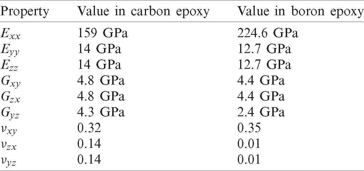
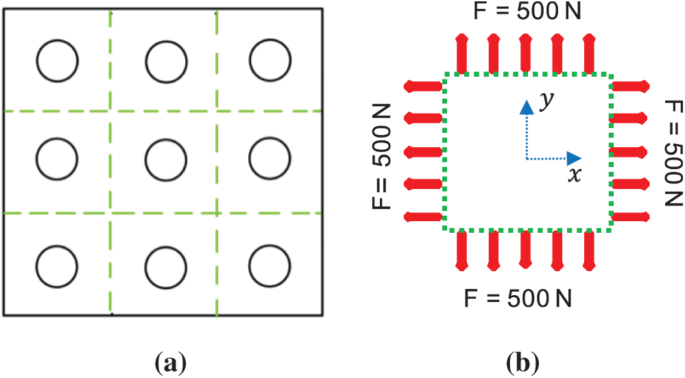
Figure 1: Geometric definition/loading condition for mechanical and thermomechanical problems. (a) Visualization of the periodic microstructure (b) mechanical problem definition using periodicity

2.1 Optimization for Mechanical Performance (Problem-1)

The first problem aims to minimize the maximum VMS value experienced by the microstructure under tensile loads (Fig. 1b). The design variables are the 9 material properties shown in Tab. 1. The optimization is performed using the Sequential Quadratic Programming (SQP) algorithm. The mathematical definition of the optimization problem is given next:

minσvonmax (2)

x=(Exx,Eyy,Ezz,Gxy,Gzx,Gyz,νxy,νzx,νyz)∈Rn(3)

The objective function is defined as the minimization of the maximum VMS value and x shows the design variables that have real values between the lower and upper bounds defined by the properties of the base materials, Carbon Epoxy and Boron Epoxy.

2.2 Optimization for Thermomechanical Performance (Problem-2)

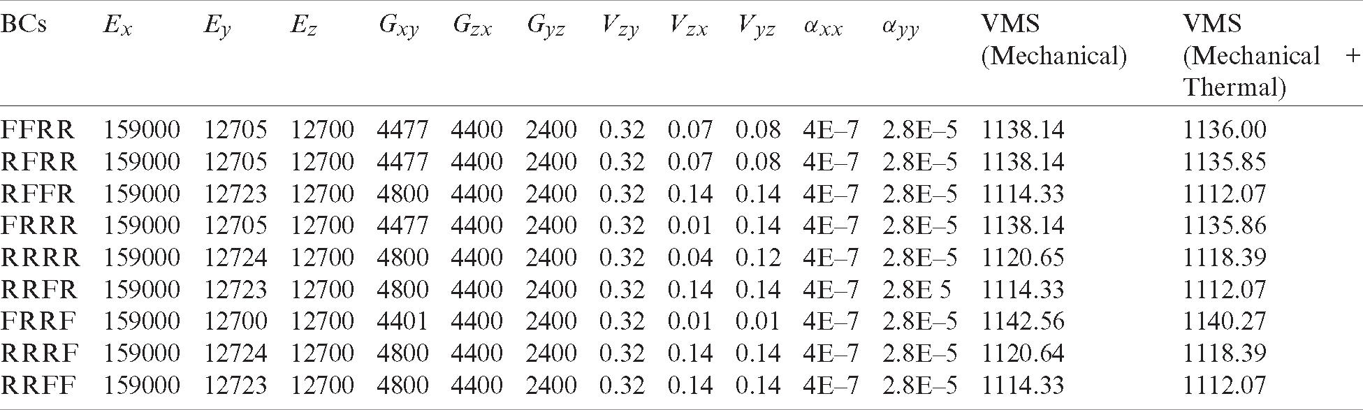
The second problem aims to minimize the maximum VMS value experienced by the microstructure under thermo-mechanical loads. The microstructure is modeled as a plate that represents a low-Earth orbit satellite component. The change of temperature is assumed to be 293 degrees according to the data presented in Reference [18]. In the optimization problem, the thermal expansion coefficients along x and y directions are defined as design variables in addition to the previous 9 material properties (Eq. (3)). The total strain is defined as the summation of the mechanical and thermal strains. The optimum results obtained with SQP for the minimization of the maximum VMS value for varying boundary conditions (BCs) can be seen in Tab. 2. The optimum VMS values are found to be around 1100 MPa for different BCs.

minσvonmax (4)

x=(Exx,Eyy,Ezz,Gxy,Gzx,Gyz,νxy,νzx,νyz,α)∈Rn(5)

Table 2: Optimum material properties of the microstructures in P1 and P2. The elastic modulus values are given in GPa, the VMS values are given in MPa, and the thermal expansion parameters are given in (1/K)

where α shows the thermal expansion tensor that includes two independent thermal expansion coefficient values, αxx and αyy. The feasible solution space for thermal expansion tensor components is constrained by the lower and upper bound values that are determined using the base materials, Carbon Epoxy and Boron Epoxy. The distributions of the VMS and thermal stress throughout the optimum microstructure designs having the roller BCs at each side of the plate in problem-1 and problem-2 are visualized in Fig. 2.

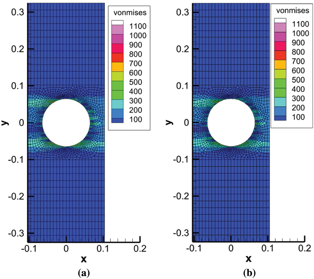
Figure 2: VMS and thermal stress distributions throughout the optimum microstructure designs that have roller BCs. (a) VMS distribution for problem-1 (b) thermal stress distribution for problem-2

2.3 Optimization for Natural Frequency (Problem-3)

The last application in this study is the optimization of the periodic microstructure to enhance the natural frequency of a plate that is assumed to be a nano-satellite component. Particularly, the natural frequency of a 2-Unit (with dimensions of 20 cm × 10 cm × 10 cm) CubeSat structure is considered. Natural frequency is an important performance metric as undesired resonance can lead to the failure of satellite components. The most important vibration implications may occur during the rocket launch. To account for the effects of the vibrations, the natural frequency of a 2-Unit CubeSat is optimized using the finite element scheme. The example CubeSat is chosen as a sample QB50 satellite of the European Union. Accordingly, the first natural frequency of a QB50 satellite should be more than 200 Hz for safety purposes [19]. The Carbon Epoxy and Boron Epoxy are used as the base materials for this 2-Unit QB50 satellite. To obtain the natural frequency value, the following dynamic system given is solved with finite element modeling.

ma+ku=md2udt2+ku=0 (4)

where m is the mass, k is the stiffness of the system, and a defines the acceleration. For the orthotropic material system, the solution of the natural frequency leads to the following expression:

ω2[m]{u}=[k]{u} (5)

Eq. (5) demonstrates an eigenvalue problem, where the eigenvalues of the system correspond to the natural frequencies of the satellite component. The frequency of the material is maximized to ensure that it is greater than 200 Hz. With the introduction of the mass matrix in the dynamic problem, one additional design variable (density of the material) is added to the optimization problem, as seen in Eq. (6) below.

minσvonmax (6)

x=(Exx,Eyy,Ezz,Gxy,Gzx,Gyz,νxy,νzx,νyz,α,ρ)∈Rn

In this equation, ρ is the material density. Similar to the other material properties, the density is allowed to acquire an optimum value that is in between the lower and upper bound values defined by the base materials. The optimum material properties that are obtained for problem-1 (P1, mechanical problem) and problem-2 (P2, mechanical + thermal problem) are the same for all different BCs and they are shown in Tab. 2. When defining BCs, F is a fixed condition and R is a roller condition. The BC determination is ordered in the clockwise direction starting from the left side of the plate. For instance, for a plate that is fixed on the left and top sides, and has rollers on the right and bottom surfaces, the BCs would be ‘FFRR’. Additionally, the optimum material properties that are obtained for problem-3 (P3, natural frequency problem) are shown in Tab. 3.

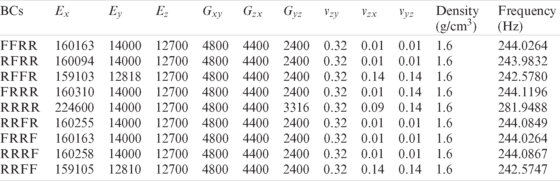
Table 3: Optimum material properties of the microstructure in P3. The elastic modulus values are given in GPa, the VMS values are given in MPa, the thermal expansion parameters are given in (1/K), and the material density is given in (g/cm3)

3  Machine Learning-Driven Design Optimization of Microstructures

To enhance the computational efficiency of the design solutions, concepts of ML (e.g., RL) are used to solve the problems involving the orthotropic material. RL is a subset of ML. It consists of an “agent” that learns how to behave in a given environment by performing actions and recording results based on those actions [20]. Multiple strategies have been utilized to solve the design problems using ML and they are discussed in this section. First, a Deep RL Neural Network is implemented to improve the computational efficiency of design optimization. Next, a Q-Value RL program is used to act as a verification code to the finite element-based design results, as well as the Deep RL network. Lastly, a feed-forward ANN is implemented to improve the computational time efficiency. The computational cost requirements for different ML techniques applied in this study are directly associated with the training data generation using finite element simulations. This is because the ML model achieve the predictions in the order of seconds with the generation of sufficient training data.

3.1 Deep Reinforcement Learning

3.1.1 Advantage Actor-Critic (A2C) Overview

The Deep RL algorithm in this work is based on the advantage actor critics RL, which is also known as Advantage Actor-Critic (A2C). Actor critics systems receive information from their external environment and select an action based on that information. After performing a specific action, the environment returns feedback, or reward in RL, to the actor. Furthermore, the critics use the state of the environment and output of the actor as its input, then evaluates how well the actor’s action is under the current environment. The critic output is similar to the reward that directly comes from the environment since both the reward and critics evaluate the actor output based on the current environment. After receiving the reward and evaluation from the critics, the actor adjusts itself and learns what action provides maximum reward under different kinds of environments. After many times of training (it took 200 iterations to train deep RL programs in this study), the actor has a very high probability of selecting the best action under a specific environment. The workflow of a Deep RL framework is shown in Fig. 3.

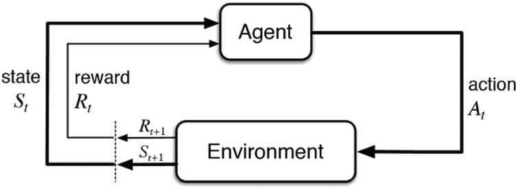
Figure 3: Workflow of a deep RL framework

3.1.2 Overall Structure of Deep RL

In this study, the material properties used in the finite element simulations define the environment for Deep RL. Deep RL starts at a random combination of material properties within the given range. The algorithm searches for the optimum combination of material properties by selecting different actions that either increase or decrease one of the material properties. After each action, the Deep RL program receives either a positive or a negative reward and then adjusts itself based on the reward so that it chooses a better action next time if it encounters a similar environment. The program selects an action, receives a reward, then adjusts itself based on the reward and selects an action again. The more iterations that the program runs, the more accurate the selected action. When the advantage is zero, RL stops adjusting itself and the combination of material properties, which is also the environment, and converges to the optimum properties.

3.1.3 Actor and Critics

The main structure of the A2C for two convolutional neural networks is defined as follows: one of the neural networks serves as an actor, and the other one serves as the critics. The actor convolution neural network has one input layer, two hidden layers, and one output layer. The inputs of the actor convolutional neural network are the material properties, which also define the environment, and the outputs of the actor are the probabilities of selecting different actions. Additionally, the critics system is designed using a convolutional neural network that consists of one input layer, one hidden layer, and one output layer. The critics network takes the actor output and current environment (material properties) as its input it outputs a Q-Value that evaluates the goodness of the actor output [20].

3.1.4 Monte Carlo Return and Neural Network Adjustment

For each action, the Deep RL receives a reward. The two convolutional neural networks can adjust themselves based on one reward from the environment, or they can adjust after selecting several actions and receiving several rewards from the environment. In this project, the one-step Monte Carlo return is chosen. In Eq. (7), the calculation of the Monte Carlo return also represents the accumulative reward after selecting one action. Here, γ is the discount factor, which is defined with a value of 0.8. This discount factor prevents the code from completely relying on future rewards. The first-order Monte Carlo Return does not have accumulative or the second reward. Consequently, the final result for Monte Carlo Return is simply the reward plus the discount factor times the next Q-Value from the critics. The advantage of the A2C scheme is that the next Q-Value is obtained with critics which makes the calculations easier.

Gt(1)=Rt+1+γvw(St+1) (7)

The goal for the adjustment of two convolution neural networks is to minimize the loss function (l). Eq. (8) shows the loss function of the critics (w) and Eq. (9) shows the loss function of the actor (θ). These two convolutional neural networks use backpropagation to adjust the weight parameters in the network.

l(w)=12(Gt(n)−vw(St))2 (8)

l(θ)=[Gt(n)−vw(St)]logπθ(At|St) (9)

3.1.5 Results for Problem-1, Problem-2, and Problem-3

In this study, the Deep RL is initialized with randomized values for properties within the ranges of base material properties. Next, the actor takes the current material properties as input and produces an output that determines whether to increase or decrease each of the material properties. Backpropagation of convolutional neural networks only takes place after receiving the reward. The design problems discussed in Section 2 are then solved using the Deep RL framework. The changes in the objective function values are shown in Figs. 4–6 for problem-1 (mechanical problem), problem-2 (thermo-mechanical problem), and problem-3 (natural frequency problem), respectively.

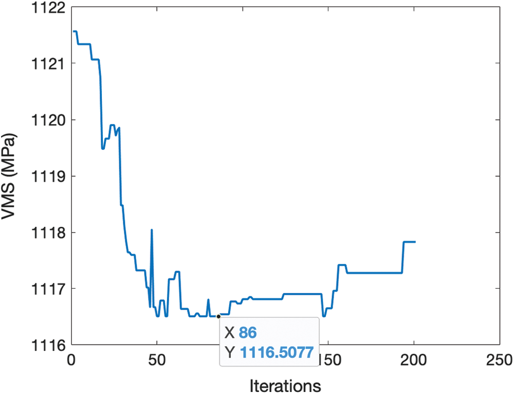
Figure 4: Changes in the objective function (VMS) obtained by deep RL in problem-1

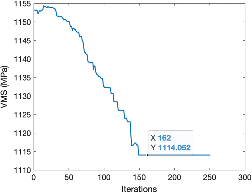
Figure 5: Changes in the objective function (VMS) obtained by deep RL in problem-2

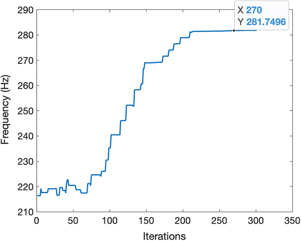
Figure 6: Changes in the objective function (natural frequency) obtained by deep RL in problem-3

In problem-1, the randomly generated initial data point provided a VMS value around 1121.5 MPa. The Deep RL successfully learned and determined the optimum choice for the material properties. Although the Deep RL aims to learn the data to make the best decision, the output of the actor is the probability of increasing or decreasing one material property, which means that there is still a small chance for the program to select a wrong action. After 200 iterations, the minimum VMS was found as 1116.507 MPa. This result is the same as the finite element-based optimization solution.

In problem-2, the final result produced by the Deep RL for VMS is 1114.1 MPa, while the finite element-based optimization solution was found as 1118.4 MPa. The Deep RL provided a better optimum solution in this problem due to the limitations arising from the gradient-based optimization algorithm (SQP) used with the finite element solution, such as the likelihood of producing local minimum solutions rather than the global solution. The gradient-based optimization is significantly dependent on the selection of the initial design point. For instance, with the change of the initial guess, the optimization result of the finite element solution also converged to 1114.1 MPa in this problem.

In problem-3, the input environment consisted of 10 variables and the output used 20 probabilities that involve increasing or decreasing material properties.

3.2 Q-Value Reinforcement Learning

3.2.1 Methodology

In this study, a value-based approach, called Q-Learning is chosen as the second RL strategy. The Q-Learning algorithm utilizes two inputs from the environment-the state and the action-and returns the expected future reward of that action and the state pair. The driving equation behind this algorithm is the Bellman Equation [21], which is shown below.

qπ(s,a)=E[Rt+1+γqπ(St+1,At+1)|St=s,At=a] (10)

The Bellman equation yields a “Q-Value,” which is a measure of the quality of performing an action at a given state. These values are stored in a Q table that is continually updated until the learning has stopped or the values have converged. The rows in the Q table are the states and the columns are the actions. The highest values in any row define the best action at that particular state.

An approach used to determine which action gets chosen at each episode in which a Q-Value is calculated is called Epsilon-Greedy. This equation is used to balance exploration-choosing actions at random- and exploitation-choosing actions based on their Q-Value. The rate of exploration is determined by the exploration rate of εthat can range from 0 to 1, with 1 meaning full exploration. After choosing an action, the action is evaluated, and the reward and next state are determined. These values are then used in the Bellman Equation (Eq. (10)).

The Q-Value RL model consists of a separate function that maps each action to the appropriate next state and objective function. The objective function given by the action is then used in a reward structure to assign the correct reward value for the action that was chosen. The next state was determined based on the action that was taken. Both the next state value and the reward value were then used to compute the Q-Value for the current state-action pair and added to the Q table. The process was repeated for 1000 iterations to allow the table to converge.

This code laid a foundational structure for the design problems involving an orthotropic material. For the first problem of finding the optimum material properties, vectors that equally distribute the range of the 9 material properties across their respective ranges were created. For computation purposes, the increments were made to only increase by a value of 20%. The Q table was set up so that each material property increment would be a state and a total of 18 actions resembled increasing or decreasing each of the 9 material properties. In this case, there were 6 total states and each odd action would increase the material property by one increment, and even actions would decrease the material property by one increment. To keep track of where each material property within their respective ranges, an index vector was created.

To map each action to the correct next state and to calculate the resulting VMS, a new function was created. This function takes in the state and action pair as well as the index vector to properly assess each state and change the index vector according to the action that was called. One important note is that this function starts the index vector according to the state that is selected. This means that if the third state is called, then all index vector entries will be the value of three. Then, based on the action value associated with a material property, the corresponding index vector will change. Since there are edge cases, the first and last states will not allow for decreasing (first state) or increasing (last state) the index vector. Each new state is the next successive state until the sixth and final state, wherein the next state is randomly chosen. Finally, the VMS is calculated based on the new set of index vector variables.

The VMS that is given by the function is used in the reward structure to aid in the calculation of the Bellman equation. It is also an integral part of the quality of the Q table that is produced. The goal of this particular problem was to find the minimized value of the maximum VMS and, thus, the reward structure had to reflect that. Two different types of reward structures were used to see the effect of reward structure on Q table quality and convergence. The first structure was a simple reward structure that would compare the new VMS value with the old VMS value. This is named the simple reward structure because the rewards are allocated using a simple principle-if the new VMS is greater than the old, a negative reward is given. Similarly, if the new VMS is less than the previous value, a positive reward is given. The other reward structure used both the previous and new, or currently calculated VMS, then used relative error to decide how rewards were given. If the relative error between the new and previous VMS values were less than or equal to 10 percent, then a positive reward was given. If the error was greater than 10 percent, then a negative reward was given. The relative error equation is given below for reference.

Relative Error=|VMSprevious−VMScurrent|VMSprevious (10)

Each of the two reward structures was compared against each other to see their effects on the Q table quality and convergence. In terms of quality, the simple reward structure gave smaller Q Values versus the relative error structure. This made distinguishing the best actions for each state a bit harder as compared to the relative error reward structure. The convergence of both structures was also very similar in that they took roughly the same amount of time to complete the desired number of iterations. Overall, they performed similarly, giving the same Q table trends when compared against each other.

The same Q-Value RL code was used to complete the second and third optimization problems for the orthotropic material. Minor adjustments were made to accommodate the new quantities, but each code is built on the same foundation of Epsilon-Greedy and a “model” function to map the states to actions of the different material properties.

The main purpose of the Q-Value RL framework is to serve as a verification tool and supplementary code that confirms results achieved through the finite element and Deep RL solutions. Rather than finding one minimized or maximized property, the Q-Value RL code serves to narrow down the range of each property value to find the optimum values to minimize VMS and maximize natural frequency. The next section discusses the results obtained by the RL Code for each of the three problems involving the orthotropic material microstructure.

3.2.2 Results for Problem-1, Problem-2, and Problem-3

The Q-Value RL framework was run for the three design problems (problem-1, problem-2, and problem-3). The optimum design parameters obtained by Q-Value RL using the RRRR boundary conditions are shown in Tabs. 4–6 for problem-1 (mechanical problem), problem-2 (thermo-mechanical problem), and problem-3 (natural frequency problem), respectively. 1000 iterations and a total of three trials were performed to find the optimum ranges for each material property.

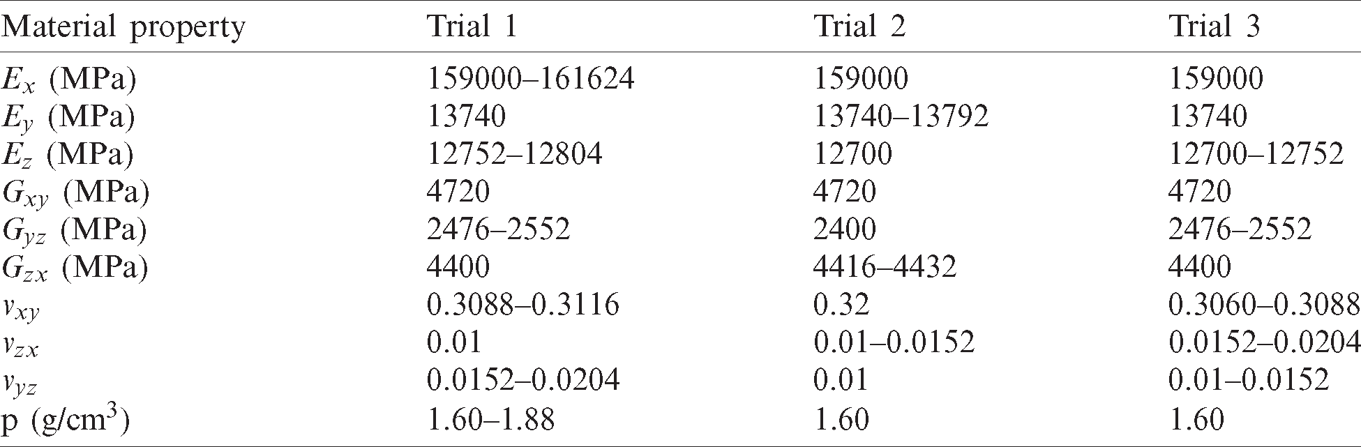
Table 4: Q-value RL results for problem-1

When comparing the results of the RL code and the optimization solution for problem-1, the results of the RL code are very similar to the finite element based optimization solution, except Gxy and νzx. This indicates that the RL code is sufficient to predict material property values for minimizing the VMS. It is suspected that the reason for the discrepancies for the Gxy and νzx values are due to their limited influence on the overall VMS value. An important note is that some trials experienced odd Q table tendencies in which there were inconclusive results. One such example is that sometimes the Q table will produce a zero value for both the increase and decrease column for some material properties. The relative error reward structure was implemented for this and all other problems were investigated. Additionally, only the RRRR boundary condition was explored in the Q-Value RL code.

For problem-2, the material properties are not quite like the results of the finite element-based optimization solution. Some material properties were close, but others varied slightly. It is believed that the reason for this discrepancy is due to the separation of the y- and z-direction values that may have caused the fluctuations in the VMS and thus caused Q Values to be manipulated.

Table 5: Q-value RL results for problem-2

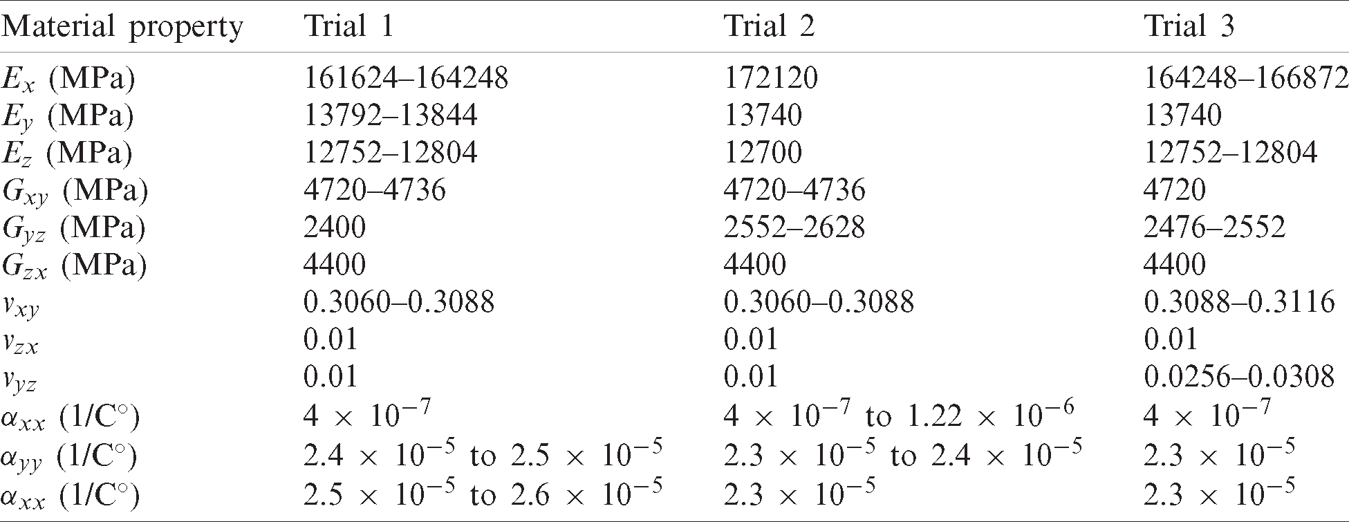
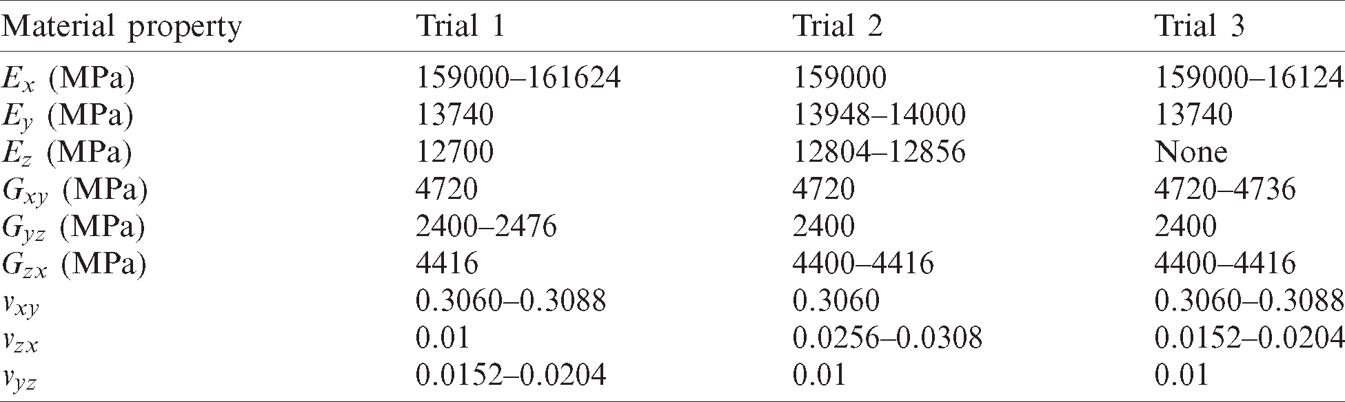
Table 6: Q-value RL results for problem-3

For problem-3, the results from the three trials show that the Q-Value RL code was able to successfully match with the optimization solution with minor discrepancies. This is mainly due to the large number of iterations showing a clear trend in the Q table for this problem.

Though the Q-Value RL code functions properly, there are still a few disadvantages of using this Q-Value RL approach to find the optimum material properties for minimizing VMS and maximizing natural frequency. The first is that the computation time using the finite element simulations is excessive. Therefore, an ANN surrogate model is utilized for this study to obtain the results with the Q-Value RL framework. Another issue is that the framework does not provide a specific value for the optimum material properties. It is only capable of showing tendencies for each material property within their respective ranges. It also does not show the minimum VMS, or maximum natural frequency, that is computed using optimum properties. Overall, it is a good validation technique for the development of more complex calculation methods and shows that rudimentary RL concepts can be applied to finite element-based design practices.

3.3 Artificial Neural Network (ANN)

3.3.1 Methodology

Due to the iterative nature of optimization solutions, design studies can require significant computational times, especially for cases that involve multi-variable, non-linear problems like the finite element modeling optimization problems in this study. Therefore, this paper investigates and compares the benefit of incorporating ANNs with different network structures to estimate optimum microstructure designs. Instead of solely using the functions generated from finite element modeling, a neural network is also implemented with the SQP algorithm to find the desired material property combinations. Then, the differences between the estimated neural network and actual optimum values are compared against each other to analyze the integrity of using artificial networks to reduce the computational times for designing multi-phase microstructures.

Before creating the neural network, 1000 sample data points are collected using the finite element model. These input data points are chosen randomly within the given material property ranges referenced in Tab. 1. Afterward, the points are used to create various training sets that contain different numbers of data points, which are chosen randomly from the original 1000 collected sample points. Within the sets, 70% of the points go to training the neural network, 15% of the points go to validation, and the other 15% go to testing. Each training set corresponds with its ANN generated by built-in MATLAB Neural Network Fitting functions. To further understand the effect of different neural networks, the study also compares different architectures containing various hidden layers and nodes to identify the most suitable structures for each problem statement.

Additionally, the actual finite element results are tested against single-layer neural networks containing 10 and 20 nodes. Similar trials are repeated with double layer networks containing 5 and 10 nodes. All neural network training is done using the Levenberg–Marquardt algorithm to fit the input and output data over 1000 epochs. Once the neural networks are trained, the function is put into an optimizer to determine the desired material property depending on the problem statement, which may utilize the maximum or minimum of the design function. For the three problems investigated in this study, the SQP algorithm was able to satisfy both conditions. Although the SQP optimizer was able to produce a result close to the actual values, it seemed to bounce between different answers depending on the initial guesses. This behavior suggested that the relationship between the material inputs and outputs contained several local minimum points, and the program would get stuck in one of them if given an uninformed initial point. Similar behavior was also referenced in the deep reinforcement algorithm discussed in Section 3.1. Thus, a GlobalSearch object was utilized to find a global minimum consistently for the optimization step of the problem.

Overall, the artificial networks were highly successful in predicting the correct output values for all three problems. In fact, after a certain number of data points in the training set, the neural networks consistently produced values within the target data. Furthermore, after running the network function into an optimizer, many of the cases had results within 1% of the expected value found from traditional methods. The best neural network architecture investigated in the study contained one layer with 20 nodes since it provided accurate results without overfitting the training data and was relatively quick to run compared to the two-layer network.

3.3.2 Results for Problem-1, Problem-2, and Problem-3

The ANN framework was run for the three optimization design problems discussed in the previous sections (Mechanical Performance, Thermo-mechanical Performance, and Natural Frequency). For problem-1, the results from optimization converged to the expected value for training sets containing around 400 data points. Problem-2 converged at around 300 data points. Finally, problem-3 converged at around 400 data points. These values suggest that to have a satisfactory artificial neural network, the training data set must be at least 400 data points. The average error and convergence of the objective functions as a function of the number of training data points is visualized in Figs. 7–9 for problem-1, problem-2, and problem-3, respectively for an ML framework consisting of one layer with 20 nodes.

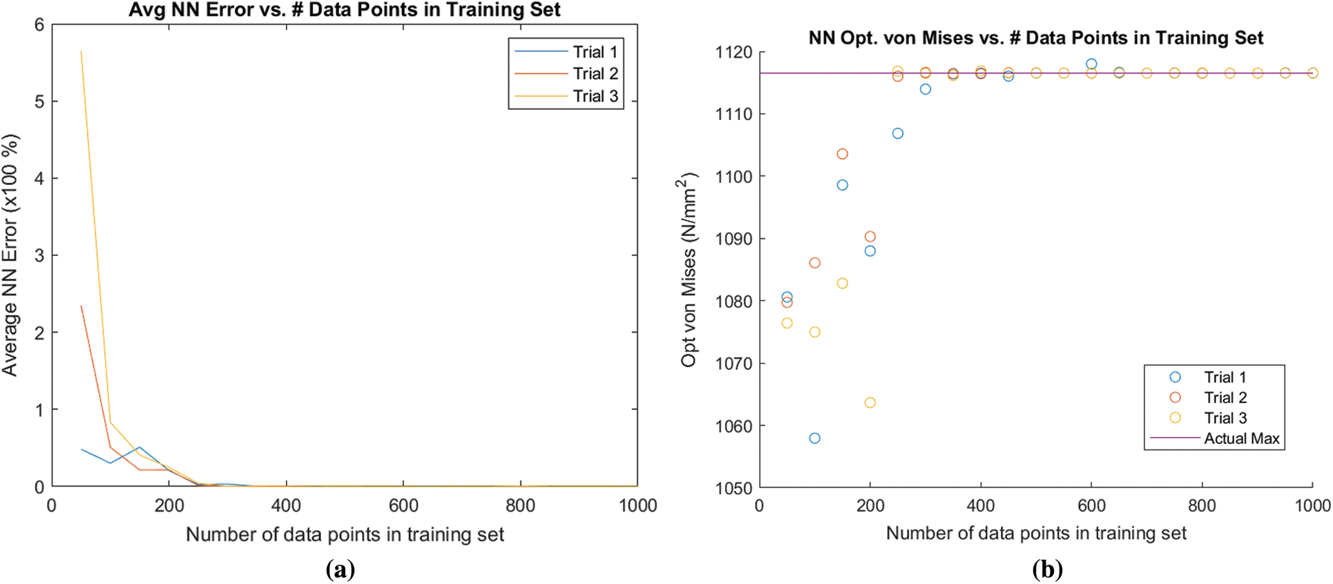
Figure 7: ANN results for problem-1 for optimization of mechanical properties. (a) Average ANN error for problem-1 (b) change in objective function for problem-1

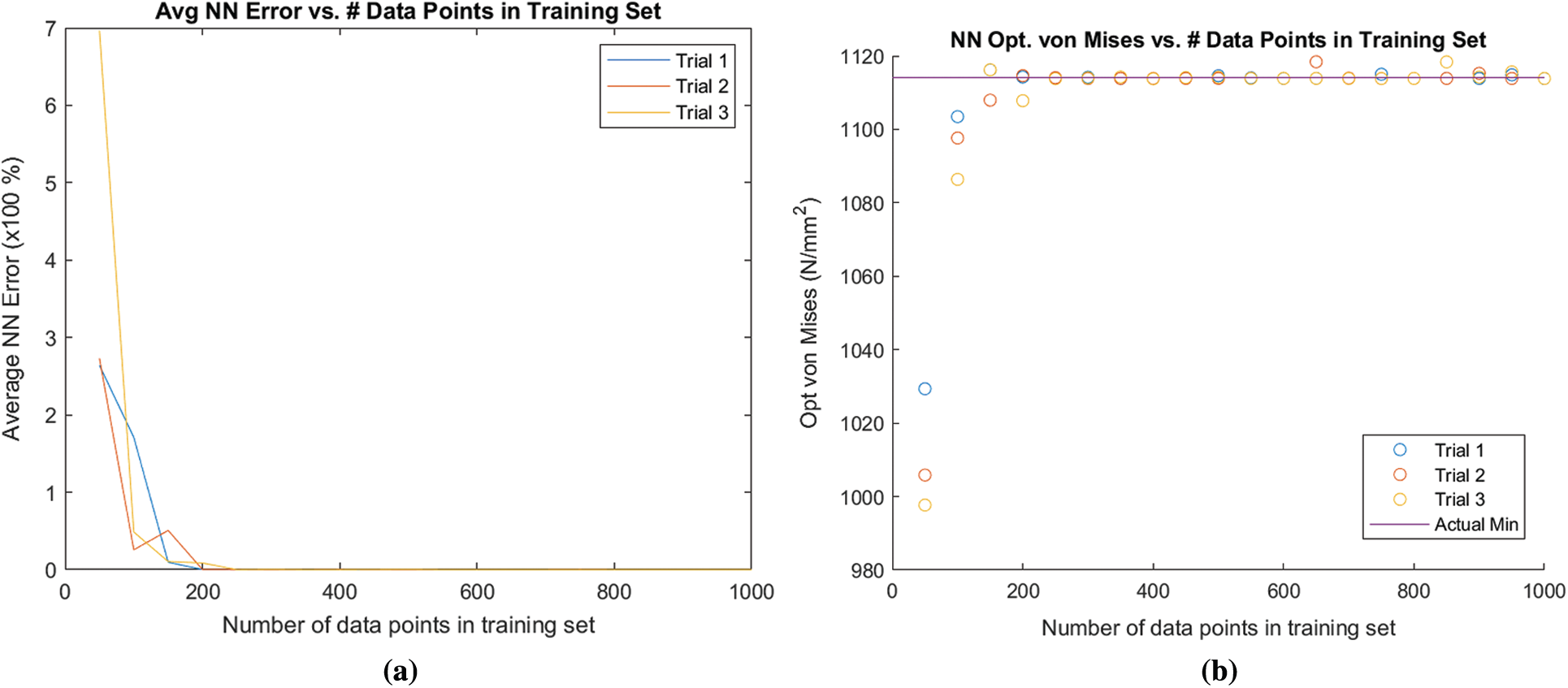
Figure 8: ANN results for problem-2 for optimization of thermo-mechanical properties. (a) Average ANN error for problem-2 (b) change in objective function for problem-2

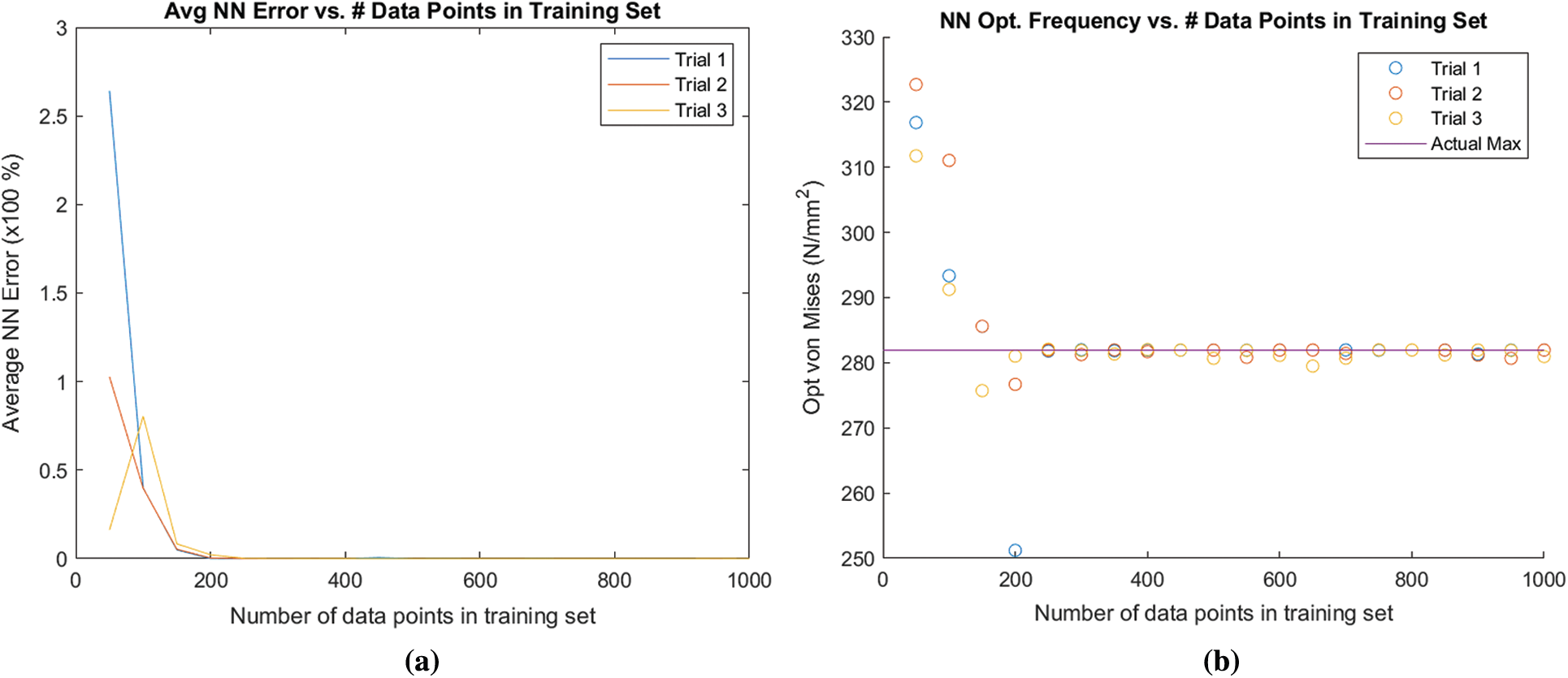
Figure 9: ANN results for problem-3 for optimization of the natural frequency. (a) Average ANN error for problem-3 (b) change in objective function for problem-3

After comparing the Q-Learning, Actor-Critic, and ANN solutions to the finite element analysis calculations, ML consistently demonstrated that artificial intelligence can accurately predict optimum results. In particular, the ANN saved much more calculation time compared to the finite element methods since it only required training one time before generating a vector function to estimate the relationship of the input and output variables. After collecting 1000 sample points for training, the framework can create and optimize 20 individual networks for 3 trials in under 10 min on a basic computational platform that utilizes a single processor. Compared to the computational times needed to run the finite element-based simulations, this new method is much faster while keeping high accuracy in the results.

4  Conclusions and Future Work

The summary of the research outcomes and potential extensions for future work are outlined below:

•       A finite element analysis library that can analyze the deformation behavior and natural frequencies of periodic microstructures under coupled mechanical and thermal loads is developed.

•       A Deep RL framework is developed and used to generate results that are compatible with the high-fidelity finite element solutions.

•       The Q-Value RL is investigated to significantly narrow down the potential solutions for optimum designs while eliminating a significantly large number of microstructural degrees of freedom.

•       An ANN framework is developed to improve the computation times of the proposed ML strategies, including the concept of Deep RL.

•       Many different settings of the proposed three ML frameworks are investigated to better understand their nature and applicability to different design problems.

The results are demonstrated for multi-phase microstructure design for various objectives, as specified in the Mechanical, Thermo-Mechanical, and Natural Frequency problems. Although the number of design variables was limited in the application problems, all different frameworks proposed and developed in this work are still applicable to the microstructure optimization problems with larger design spaces. Therefore, the future work for this topic will include an increased focus on the extension of the presented ML-driven design strategy to optimize multi-phase materials in larger length-scales by utilizing solution spaces that involve millions of variables.

Funding Statement: The presented work was funded by the NASA Virginia Space Grant Consortium Grant (Project Title: “Deep Reinforcement Learning for De-Novo Computational Design of Meta-Materials”).

Conflicts of Interest: The authors declare that they have no conflicts of interest to report regarding the present study.

This work is licensed under a Creative Commons Attribution 4.0 International License, which permits unrestricted use, distribution, and reproduction in any medium, provided the original work is properly cited.