Computers, Materials & Continua DOI:10.32604/cmc.2021.016600
Article

Computer Vision-Control-Based CNN-PID for Mobile Robot

Rihem Farkh1,5,*, Mohammad Tabrez Quasim2, Khaled Al jaloud1, Saad Alhuwaimel3 and Shams Tabrez Siddiqui4

1College of Engineering, Muzahimiyah Branch, King Saud University, P.O. Box 2454, Riyadh, 11451, Saudi Arabia
2College of Computing and Information Technology, University of Bisha, Bisha, 67714, Saudi Arabia
3King Abdulaziz City for Science and Technology, Saudi Arabia
4Department of Computer Science, College of Computer Science and Information Technology, Jazan University, Jazan, Saudi Arabia
5Department of Electrical Engineering, Laboratory for Analysis, Conception and Control of Systems, LR-11-ES20, National Engineering School of Tunis, Tunis El Manar University, Tunis, Tunisia
*Corresponding Author: Rihem Farkh. Email: rfarkh@ksu.edu.sa
Received: 06 January 2021; Accepted: 07 February 2021

Abstract: With the development of artificial intelligence technology, various sectors of industry have developed. Among them, the autonomous vehicle industry has developed considerably, and research on self-driving control systems using artificial intelligence has been extensively conducted. Studies on the use of image-based deep learning to monitor autonomous driving systems have recently been performed. In this paper, we propose an advanced control for a serving robot. A serving robot acts as an autonomous line-follower vehicle that can detect and follow the line drawn on the floor and move in specified directions. The robot should be able to follow the trajectory with speed control. Two controllers were used simultaneously to achieve this. Convolutional neural networks (CNNs) are used for target tracking and trajectory prediction, and a proportional-integral-derivative controller is designed for automatic steering and speed control. This study makes use of a Raspberry PI, which is responsible for controlling the robot car and performing inference using CNN, based on its current image input.

Keywords: Autonomous car; pid control; deep learning; convolutional neural network; differential drive system; raspberry pi

1  Introduction

From the automobile to pharmaceutical industries, traditional robotic manipulators have been a popular manufacturing method for various industries for at least two decades. Additionally, scientists have created many different forms of robots other than traditional manipulators to expand the use of robotics. The new types of robots have more freedom of movement, and they can be classified into two groups: redundant manipulators and mobile (ground, marine, and aerial) robots. Engineers have had to invent techniques to allow robots to deal automatically with a range of constraints. Robots that are equipped with these methods are called autonomous robots [1].

Mobile robots can move from one location to another to perform desired tasks that can be complex [2]. A mobile robot is a machine controlled by software and integrated sensors, including infrared, ultrasonic, webcam, GPS, and magnetic sensors. Wheels and DC motors are used to drive robots through space [3]. Mobile robots are often used for agricultural, industrial, military, firefighting, and search and rescue applications (Fig. 1), allowing humans to accomplish complicated tasks [4].

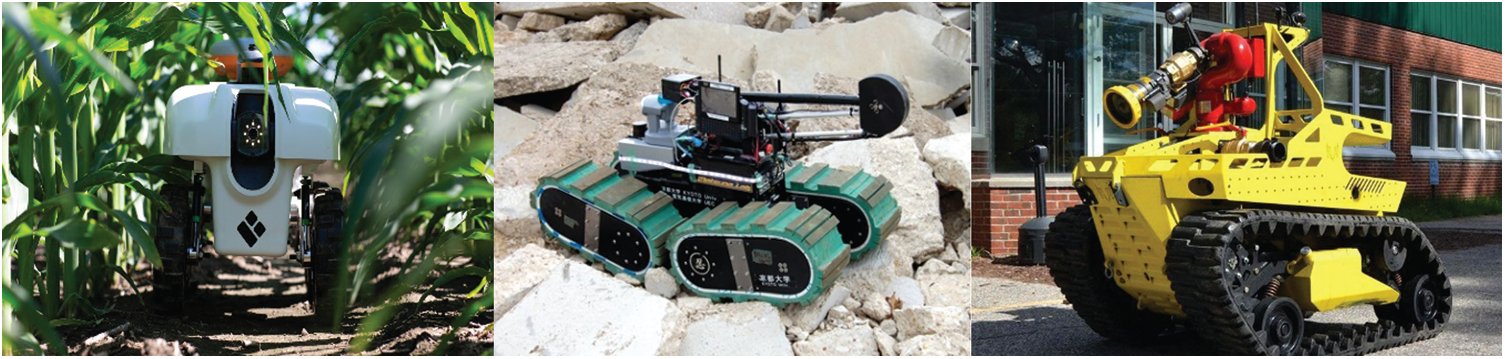
Figure 1: Autonomous robots

Line-follower robots can be used in many industrial logistics applications, such as transporting heavy and dangerous material, the agriculture sector, and library inventory management systems (Fig. 2). These robots are also capable of monitoring patients in hospitals and warning doctors of dangerous symptoms [5].

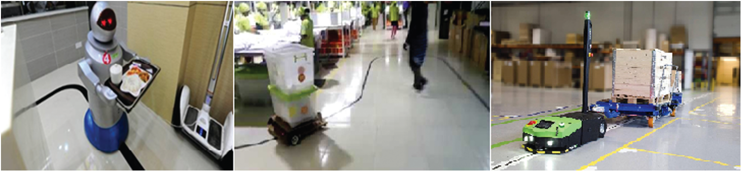
Figure 2: Line-follower serving robots

A substantial number of researchers have focused on smart-vehicle navigation because of the limitations of traditional tracking techniques due to the environmental instability under which vehicles move. Therefore, intelligent control mechanisms, such as neural networks, are needed, as they provide an effective solution to the problem of vehicle navigation due to their ability to learn the non-linear relationship between input and sensor variables. A combination of computer vision techniques and machine learning algorithms are necessary for autonomous robots to develop “true consciousness” [6]. Several attempts have been made to improve low-cost autonomous cars using different neural-network configurations, including the use of a convolutional neural network (CNN) for self-driving vehicles [7]. A collision prediction system was constructed using a CNN, and a method was proposed for stopping a robot in the vicinity of the target point while avoiding a moving obstacle [8]. A CNN has also been proposed for keeping an autonomous driving control system in the same lane [9], and a multilayer perceptron network has been used for mobile-robot motion planning [10]. It was implemented on a PC Intel Pentium 350 MHz processor. Additionally, the problem of navigating a mobile robot has been solved by using a local neural-network model [11].

A variety of motion control methods have been proposed for autonomous robots: proportional-integral-derivative (PID) control, fuzzy control, neural network control, and some combination of these control algorithms [12]. The PID control algorithm is used by most motion control applications, and PID control methods have been extended with deep learning techniques to achieve better performance and higher adaptability. Highly dynamic high-end robotics with reasonably high accuracy of movement almost always require these control algorithms for operation. For example, a fuzzy PID controller for electric drives for a differential drive autonomous mobile robot trajectory application has been developed [13]. Additionally, a PID controller for a laser sensor-based mobile robot has been designed to detect and avoid obstacles [14].

In this paper, the low-cost implementation of a combined PID controller with a CNN is realized using the raspberry pi platform for the smooth control of an autonomous line-follower robot.

2  Autonomous Line-Follower Robot Architecture

In this Section, the architecture and system block are described. First, a suitable configuration was selected to develop a line-follower robot using a Pi camera connected through a Raspberry Pi3 B+ to the motor driver IC. This configuration is illustrated in the block diagram shown in Fig. 3.

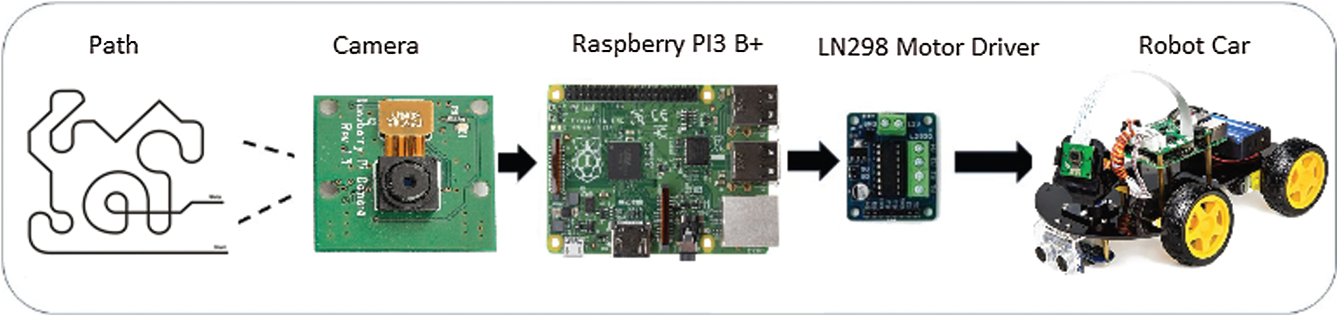
Figure 3: Block diagram of the line-follower robot

Implementing the system on the Arduino Uno ensured the following:

•      moving the robot in the desired direction;

•      collecting data from the Pi camera and feeding it into a CNN;

•      predicting the error between the path line and the robot position;

•      determining the speed of the left and right motors using a PID controller and the predicted error;

•      operating the line-follower robot by controlling the four DC motors; and

•      avoiding obstacles using an ultrasonic sensor.

2.1 Mobile-Robot Construction

The proposed mobile-robot design can easily be adapted to new and future research studies. The physical appearance of the robot was evaluated, and its design was based on several criteria, including functionality, material availability, and mobility. During the analysis of different guided robots of reduced size and simple structure (as shown in Fig. 4), the work experience of the authors with mechanical structures for robots was also considered.

Seven types of parts were used in the construction of the robot:

1.    Four wheels,

2.    Four DC motors,

3.    Two base structures,

4.    A control board formed using the Raspberry Pi3 B+ board,

5.    An LN298 IC circuit for DC-motor driving,

6.    An expansion board, and

7.    An ultrasonic sensor HC-SR04.

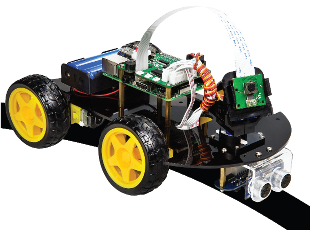
Figure 4: Line-follower robot prototype

2.2 Raspberry Pi Camera

The Raspberry Pi camera module is a light-weight, compact camera that supports the Raspberry Pi (Fig. 5). Using the MIPI camera serial interface protocol, it communicates with the Raspberry Pi. It is usually used in machine learning, processing images, or security projects. The Raspberry Pi camera module is connected to the CSI port of Raspberry Pi. When the Raspberry Pi camera starts and is logged into the desktop typing the raspistill–o image.jpg command in prompt and pressing enter stores the image as image.jpg, which can be viewed in GUI and confirms the running of the Raspberry Pi camera. Python script is used to control the Raspberry Pi camera and capture the image [15].

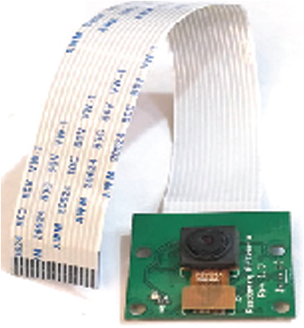
Figure 5: The raspberry Pi camera

2.3 Obstacle Detector

The HC-SR04 ultrasonic sensor uses sonar to determine the distance from it to an object (Fig. 6). It offers excellent non-contact range detection with high accuracy and stable readings in an easy-to-use package. It comes complete with ultrasonic transmitter and receiver modules [16]. Below is a list of some of its features and specs:

•      Power Supply: +5 V DC

•      Quiescent Current: < 2 mA

•      Working Current: 15 mA

•      Effectual Angle: < 15∘

•      Ranging Distance: 2 −400 cm/1′-13ft

•      Resolution: 0.3 cm

•      Measuring Angle: 30 degree

•      Trigger Input Pulse width: 10 uS

•      Dimension: 45mm×20mm×15mm

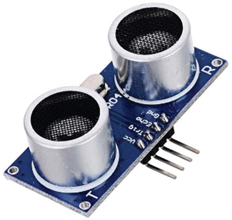
Figure 6: Ultrasonic sensor HC-SR04

2.4 Raspberry Pi 3B+

The Raspberry Pi is an inexpensive, credit-card-sized single board computer developed in the United Kingdom by the educational charity, the Raspberry Pi Foundation (Fig. 7). The Raspberry Pi 3 Model-B is the 3rd generation Raspberry Pi minicomputer with a 64-bit 1.2 GHz quad-core processor, 1GB RAM, WiFi, and Bluetooth 4.1 controllers. It also has 4× USB 2.0 ports, 10/100 Ethernet, 40 GPIO pins, a full-size HDMI 1.3a port, camera interface (CSI), combined 3.5 mm analog audio and composite video jack, a display interface (DSI), MicroSD slot, and VideoCore IV multimedia/3D graphics core@400 MHz/300 MHz [17].

The GPIO27 (Physical pin 13) and the GPIO22 (Physical pin 15) are connected to IN1 and IN2 of the L298N module, respectively, to drive the left motors. The GPIO20 (Physical pin 38) and the GPIO21 (Physical pin 40) are connected to IN3 and IN4 of the L298N module respectively, to drive the right motors.

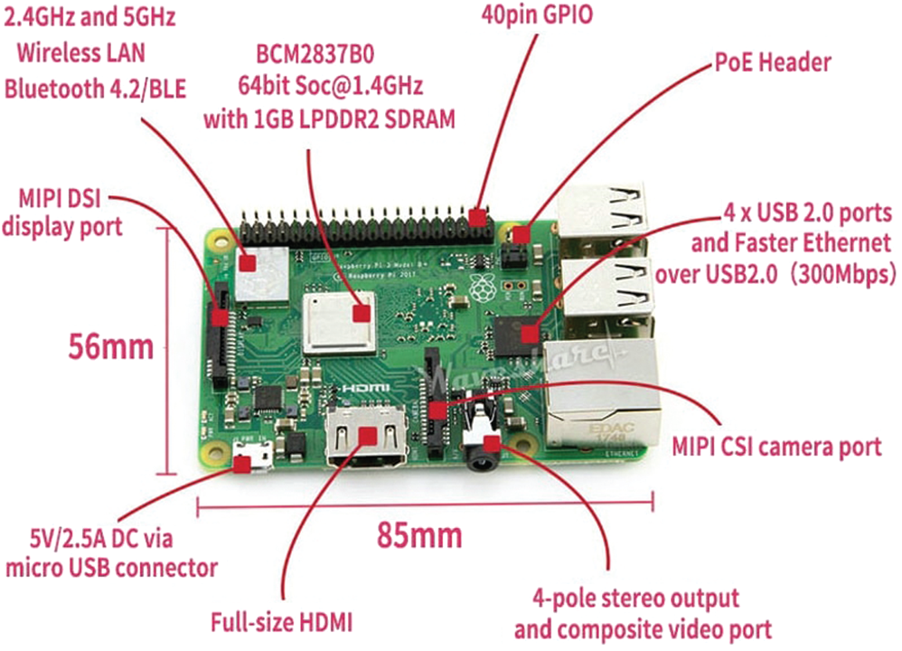
Figure 7: Raspberry Pi 3B+ board

2.5 L298N Motor Driver

The L298N motor driver (Fig. 8) consisted of two complete H-bridge circuits. Thus, it could drive a pair of DC motors. This feature makes it ideal for robotic applications because most robots have either two or four powered wheels operating at a voltage between 5 and 35 V DC with a peak current of up to 2A. This module incorporated two screw-terminal blocks for motors A and B and another screw-terminal block for the ground pin, the VCC for the motor, and a 5-V pin, which can either be an input or output. The pin assignments for the L298N dual H-bridge module are shown in Tab. 1. The digital pin, which is assigned from HIGH to LOW or LOW to HIGH, was used for the IN1 and IN2 on the L298N board to control the direction. The controller output PWM signal was sent to the ENA or ENB to control the position. The forward and reverse speed or position control of the motor was achieved using a PWM signal [18]. Then, using the analogWrite() function, the PWM signal was sent to the Enable pin of the L298N board, which drives the motor.

Figure 8: LN298 IC motor driver

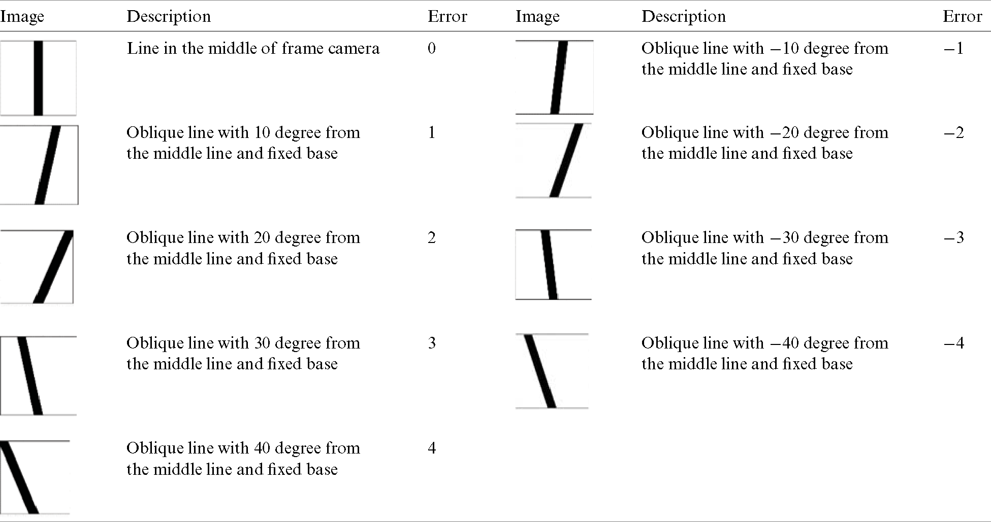
Table 1: Errors and line positions in the camera frame

3  Convolutional-Neural-Network-Based Proportional Integral Derivative Controller Design for Robot Motion Control

A PID-based CNN controller was designed to control the robot. An error value of zero referred to the robot being precisely in the middle of the image frame. Error is assigned for each line position in the camera frame image, as explained Tab. 1.

A positive error value meant that the robot had deviated to the left and a negative error value meant that the robot had deviated to the right. The error had a maximum value of ±4, which corresponds to the maximum deviation.

Tab. 2 presents the assignment of errors to real images tacked with the Raspberry Pi camera.

Table 2: Errors and real line positions in the Raspberry Pi camera frame

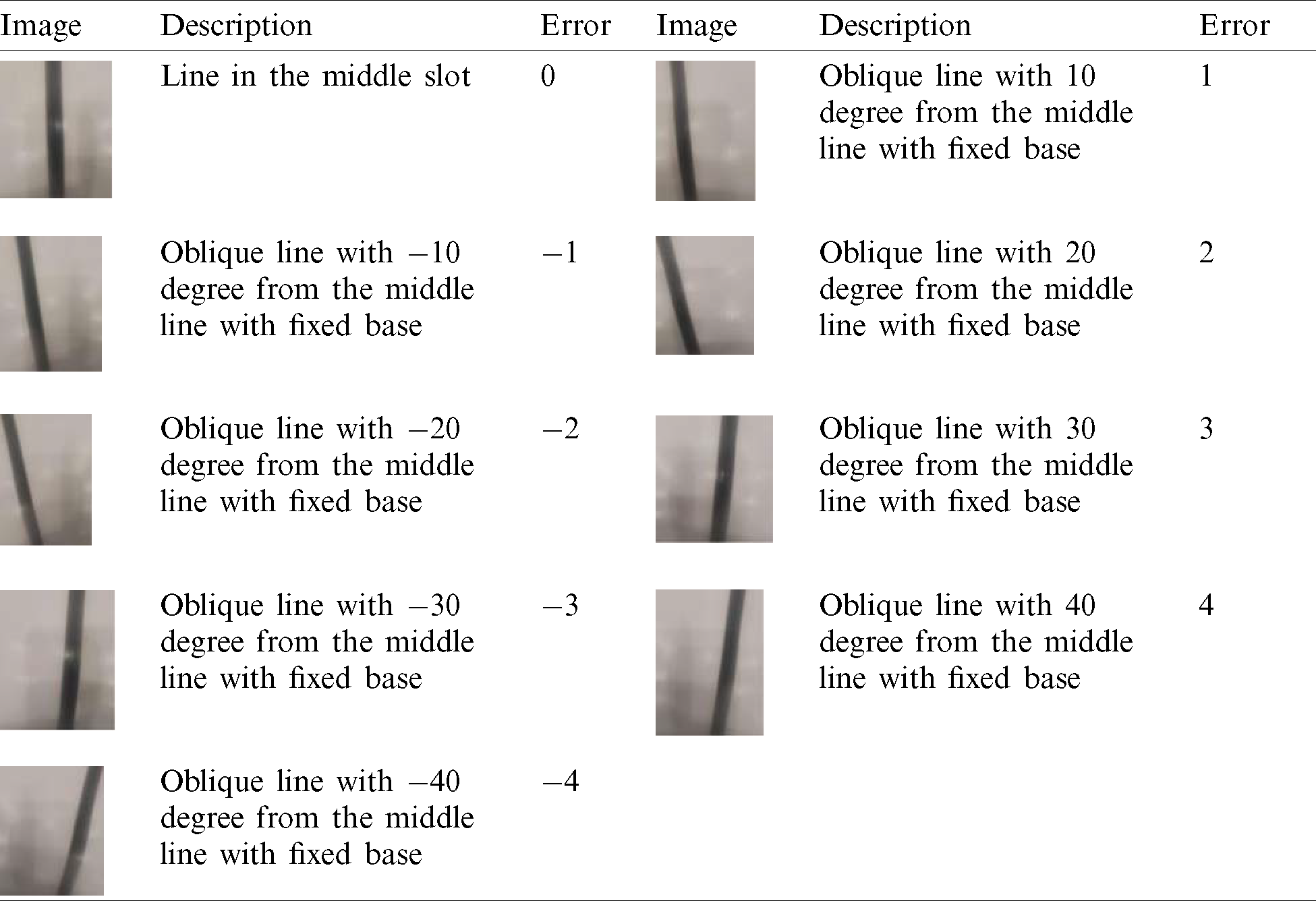
The primary advantage of this approach is extracting the error from the image given by the Raspberry Pi camera, which can be fed to the controller to compute the motor speeds such that the error term becomes zero.

The estimated error input was used by the PID controller to generate new output values (control signal). The output value was exploited to determine the Left Speed and Right Speed for the two motors on the line-follower robot.

Fig. 9 presents the control algorithm used for the line-follower robot.

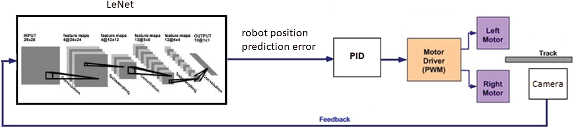
Figure 9: Proportional-integral-derivative and convolutional neural network deep-learning control

3.1 Proportional-Integral-Derivative Control

A PID controller aims to keep an input variable close to the desired set-point by adjusting an output. This process can be ‘tuned’ by adjusting three parameters: KP, KI, KD. The well-known PID controller equation is shown here in continuous form

Uc(t)=Kpe(t)+Ki∫e(t)dt+Kdde(t)dt where Kp, Ki, and Kd refer to proportional, integral, and derivative gain constants respectively.

For implementation in a discrete form, the controller equation is modified by using the backward Euler method for numerical integration. u(kT)=Kpe(kT)+KiT∑kne(kT)+Kde(kT)-e(kT-T)T where u(kT)and e(kT) are control signal and error signal in discrete-time at T sampling time.

The PID controls both the left and right motor speeds according to predicted error measurement of the sensor. The PID controller generates a control signal (PID-value), which is used to determine the left and the right speed of robot wheels.

It is a differential drive system: a left turn is achieved if the speed of the left motor is reduced, and a right turn is achieved if the speed of the right motor is reduced. RightSpeed=Base-speed-PID-valueLeftSpeed=Base-speed+PID-value

Right speed and left speed are used to control the duty cycle of the PWM applied at the input pins of the motor driver IC.

The PID constants (Kp, Ki, Kd) were obtained using the Ziegler–Nichols tuning method [19]. To start, the Ki and Kd of the system was set to 0. Then, the Kp was increased from 0 until it reached the ultimate gain Ku, and at this point, the robot continuously oscillated. The Ku and Tu (oscillation period) were then used to tune the PID (see Tab. 3).

Table 3: Proportional-integral-derivative control tuning parameters

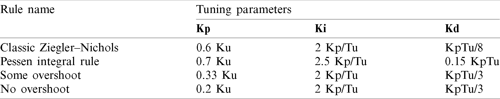
According to substantial testing, using a classical PID controller was unsuitable for the line-follower robot because of the changes in line curvature. Therefore, only the last three error values were summed up instead of adding all the previous values to solve this problem. The modified controller equation is given as

u(kT)=Kpe(kT)+KiT∑k3e(kT)+Kde(kT)-e(kT-T)T

This technique provides satisfactory performance for path tracking.

3.2 LeNet Convolutional Neural Networks

The use of CNNs is a powerful artificial neural network technique. CNNs are multilayer neural networks built especially for 2D data, such as video and images, and they have become ubiquitous in the area of computer vision. These networks maintain the spatial structure of the problem, make efficient use of patterns and structural information in an image, and have been developed for object recognition tasks [20].

CNNs are so named due to the presence of convolutional layers in their construction. The detection of certain local features in every location of the particular input image is the primary work of the convolutional layers. The convolution layer comprises a set of independent filters. The filter is slid over the complete image and the dot product is taken between the filter and chunks of the input image. Each filter is independently convolved with the image to end up with feature maps. There are several uses that we can gain from deriving a feature map and reducing the size of the image by preserving its semantic information is one of them.

In this paper, we propose using the LeNet CNN (Fig. 10) to take advantage of it ability to classify small single-channel (black and white) images. LeNet was proposed in 1989 by Yann et al. [21], and it was later widely used in the recognition of handwritten characters. He combined a CNN trained to read black lines using backpropagation algorithms. LeNet has the essential basic units of CNN, such as a convolutional layer, pooling layer, and full connection layer. The convolution kernels of the three convolutional layers are all 5×5, and the activation function uses the Sigmoid function.

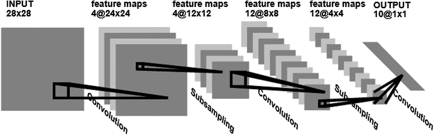
Figure 10: The LeNet convolutional neural network structure

The LeNet CNN included five layers and configured them to process single-channel scale images of size (28×28):

•      Layer C1: Convolution layer (numberofkernels=4, kernel_size=5×5, padding=0, stride=1)

•      Layer S2: Average pooling layer (kernel_size=2×2, padding=0, stride=2)

•      Layer C3: Convolution layer (numberofkernels=12, kernel_size=5×5, padding=0, stride=1)

•      Layer S4: Average pooling layer (kernel_size=2×2, padding=0, stride=2)

•      Layer F5: Fully connected layer (out_features=10)

The input for the LeNet CNN is a 28×28 grayscale image, which passes through the first convolutional layer with four feature maps or filters with a size of 5×5 and a stride of one. The image dimensions change from 28×28×1 to 24×24×4. Then, the LeNet applies an average pooling layer or sub-sampling layer with a filter size of 2×2 and a stride of two. The resulting image dimensions are reduced to 12×12×4. Next, there is a second convolutional layer with 12 feature maps with a size of 8×8 and a stride of 1. In this layer, only 8 out of 12 feature maps are connected to four feature maps of the previous layer. The fourth layer (S4) is again an average pooling layer with a filter size of 2×2 and a stride of two. This layer is the same as the second layer (S2) except it has 12 feature maps, so the output is reduced to 4×4×12. The fifth layer (F5) is a fully connected softmax layer with 10 feature maps each of a size of 1×1 with 10 possible values corresponding to the digits from 0 to 9.

4  Implementation on Raspberry Pi

A substantial amount of data are required to create a neural network model. These data are gathered during the training process. Initially, the robot has to be wirelessly operated using the VNC Viewer, which helps monitor the Raspberry Pi through Wi-fi. As the robot is run on the path line it collects image data through the Raspberry Pi camera. These data are used to train the LeNet neural network model.

The script for the CNN algorithm was developed in Python [22]. This code was transported to the RP via a virtual development environment provided by the Python language composed of the interpreter, libraries, and scripts. Each project implemented on either the computer or Raspberry depends on the Python virtual development environment without affecting dependence on other projects. The dependencies in the RP virtual environment for running the training and test applications include Python 3, OpenCV, NumPy, Keras, and TensorFlow.

To capture a set of images at an interval of 0.5 s, we used the pseudo code listed in the figure below:

from picamera.array import PiRGBArray

from picamera import PiCamera

import time

import cv2

camera=PiCamera( )camera.resolution = (640, 480)

camera.framerate = 32

rawCapture = PiRGBArray (camera, size = (640, 480))

time.sleep (0.1)

start = 1

for frame in camera.capture_continuous (rawCapture, format =“bgr, ”use_video_port = True) :

image= frame.array

cv2.imshow(“Frame, ”image)

key =cv2.waitKey(1)

cv2.imwrite (str (start)+“.jpg, ” image)

start = start +1

if key == ord (“q”) : breaktime.sleep (.5)

Once the images were captured for many positions of the robot on the track, they were placed in different folders. We trained our LeNet system on the images captured using the following code. However, first we imported the necessary libraries, such as Numpy, cv2, and Matplotlib.

class LeNet:

@staticmethod

def build (width, height, depth, classes) :

model = Sequential () inputShape =(height, width, depth)

model.add (Conv2D(20, (5, 5) , padding =“same, ”input_shape =inputShape))

model.add (Activation (“relu”))

model.add (MaxPooling2D(pool_size =(2, 2), strides=(2, 2)))

model.add (Conv2D(50, (5, 5) , padding =“same”))

model.add (Activation (“relu”))

model.add (MaxPooling2D(pool_size =(2, 2), strides=(2, 2)))

model.add (Flatten ())

model.add (Dense (500))

model.add (Activation (“relu”))

model.add (Dense (classes))

model.add (Activation (“softmax”))

return model

The path of each image present in subfolders is registered, stored in the imagePath list, and shuffled. Shuffling is expected to provide data randomly from each class when training the model. Additionally, each image is then read, resized, converted into Numpy array and stored in data, and each image is given a label.

The folder name is extracted from the image path of each image. A label of 0 is assigned if the folder name is “error=0.” Similarly, a label of −4, −3, −2, −1, 1, 2, 3, 4 is assigned to images present in folder “error=-4,” “error=-3,” folder “error=-2,” folder “error=-1,” folder “error=1,” folder “error=2,” folder “error=3,” and folder “error=4.”

dataset = ′/home/pi/Desktop/tutorials/raspberry/trainImages/′

data = [ ]

labels = [ ]

imagePaths = sorted (list (paths.list_images (dataset)))

random.seed (42) random.shuffle (imagePaths)

for imagePath in imagePaths :

image = cv2.imread(imagePath)

image = cv2.resize (image, (28, 28))

image = img_to_array (image)

data.append (image)

label = imagePath.split (os.path.sep) [−2] print (label)

if label ==′ error =−4′: label =−4

elif label ==′ error =−3′: label =−3

elif label ==′ error =−2′: label =−2

elif label ==′ error =−1′: label =−1

elif label ==′ error =0′: label =0

elif label ==′ error =+1′: label = +1

elif label ==′ error =+2′: label = +2

elif label ==′ error =+3′: label = +3

else : label =+4

labels.append (label)

The images are normalized and each of the pixel values is between 0 and 1. Then, the images are separated into a training set and test set to validate the performance of the model. Next, the LeNet class was used to construct the model using the training data.

data = np.array (data, dtype = “float”) /255.0

labels = np.array (labels)

(trainX, testX, trainY, testY) = train_test_split (data, labels, test_size = 0.25, random_state = 42)

trainY = to_categorical (trainY, num_classes = 3) testY = to_categorical (testY, num_classes = 3)

EPOCHS = 15

INIT_LR = 1e−3

BS = 32

print (“ [INFO] compiling model… ”)

model = LeNet.build (width = 28, height = 28, depth = 3, classes = 3)

opt = Adam(lr = INIT_LR, decay =INIT_LR / EPOCHS)

model.compile (loss = “binary_crossentropy, ”

optimizer = opt,metrics = [“accuracy”])

print (“ [INFO] training network… ”)

H = model.fit (trainX, trainY, batch_size = BS,

validation_data = (testX, testY) ,BS, epochs = EPOCHS, verbose =1)

print (“ [INFO] serializing network… ”)

model.save (“model”)

Once the model is trained, it can be deployed on the Raspberry Pi. The code below was used to control the robot, based on the prediction from the LeNet CNN and the PID controller. A PID controller continuously calculates an error and applies a corrective action to resolve it. In this case, the error is the position prediction delivered by the CNN and the corrective action is changing the power to the motors. We defined a function PID_control_robot that will control the direction of the robot based on prediction from the model.

def PID_control_robot (image) :

error_predection = np.argmax(model.predict (image))

Pid_adjustement = PID (Error_predection)

Right_speed = Base_speed + Pid_adjustement

Left_speed = Base_speed − Pid_adjustement

5  Conclusions

We presented a vision-based, self-driving robot, in which an image input is taken through the camera and a CNN model is used to take a decision accordingly. We developed and a combined a PID and CNN deep-learning controller to guaranty a smooth tracking line. The results indicated that the proposed method is well suited to mobile robots, as they are capable of operating with imprecise information. More advanced controller-based CNNs could be developed in the future.

Acknowledgement: The authors acknowledge the support of King Abdulaziz City of Science and Technology.

Funding Statement: The authors received no specific funding for this study.

Conflicts of Interest: The authors declare that they have no conflicts of interest to report regarding the present study.

This work is licensed under a Creative Commons Attribution 4.0 International License, which permits unrestricted use, distribution, and reproduction in any medium, provided the original work is properly cited.