DOI:10.32604/cmc.2021.016536
| Computers, Materials & Continua DOI:10.32604/cmc.2021.016536 | |
| Article |
Evolutionary GAN–Based Data Augmentation for Cardiac Magnetic Resonance Image
1School of Computer Science, Chengdu University of Information Technology, Chengdu, 610225, China
2Images and Spatial Information 2011 Collaborative Innovation Center of Sichuan Province, Chengdu, 610225, China
3Department of Computer Science, University of Reading, Earley, RG6 6AY, UK
*Corresponding Author: Ying Fu. Email: fuying@cuit.edu.cn
Received: 04 January 2021; Accepted: 09 February 2021
Abstract: Generative adversarial networks (GANs) have considerable potential to alleviate challenges linked to data scarcity. Recent research has demonstrated the good performance of this method for data augmentation because GANs synthesize semantically meaningful data from standard signal distribution. The goal of this study was to solve the overfitting problem that is caused by the training process of convolution networks with a small dataset. In this context, we propose a data augmentation method based on an evolutionary generative adversarial network for cardiac magnetic resonance images to extend the training data. In our structure of the evolutionary GAN, the most optimal generator is chosen that considers the quality and diversity of generated images simultaneously from many generator mutations. Also, to expand the distribution of the whole training set, we combine the linear interpolation of eigenvectors to synthesize new training samples and synthesize related linear interpolation labels. This approach makes the discrete sample space become continuous and improves the smoothness between domains. The visual quality of the augmented cardiac magnetic resonance images is improved by our proposed method as shown by the data-augmented experiments. In addition, the effectiveness of our proposed method is verified by the classification experiments. The influence of the proportion of synthesized samples on the classification results of cardiac magnetic resonance images is also explored.
Keywords: Evolutionary generative adversarial network; cardiac magnetic resonance; data augmentation; linear interpolation
Cardiac magnetic resonance imaging (MRI) is the gold standard for assessing cardiac function. Conventional cardiac MRI scanning technology has advanced over the years and plays a vital role in the diagnosis of disease. Currently, many cardiac magnetic resonance image-assisted diagnosis tasks that are based on deep learning [1] have achieved good results. A novel algorithm [2] was proposed by Renugambal et al. for multilevel thresholding brain image segmentation in magnetic resonance image slices. This approach requires expensive medical equipment to obtain cardiac magnetic resonance images and also needs experienced radiologists to label them manually. It is undoubtedly extremely time-consuming and labor-intensive. The privacy of patients in the field of medical imaging has always been very sensitive and it is expensive to obtain a large number of datasets that are balanced between positive and negative samples.
A significant challenge in the field of medical imaging based on deep learning is how to deal with small-scale datasets and a limited number of labeled data. Datasets are often not sufficient or the dataset sample is unbalanced, especially when using a complex deep learning model, which makes the deep convolution neural network with a huge number of parameters appear as overfitting [3]. In the field of computer vision, scholars have proposed many effective methods for overfitting, such as batch regularization [4], dropout [5], early stopping method [6], weight sharing [7], weight attenuation [8], and others. These methods are to adjust the network structure. Data augmentation [9] is an effective method to operate on the data itself, which alleviates to a certain extent the problem of overfitting in image analysis and classification. The classical data augmentation techniques mainly include affine transformation methods such as image translation, rotation, scaling, flipping, and shearing [10,11]. These approaches mix the original samples and new samples as training sets and input them into a convolutional neural network. The adjustment of the color space of samples is also a data augmentation method. Sang et al. [12] used the method of changing the brightness value to expand the sample size. These methods have improved solving the overfitting problem. However, the operation on the original samples does not produce new features. The diversity of the original samples has not been substantially increased [13], and the promotion effect is weak when processing small–scale data. Liu et al. [14] used a data augmentation method on the test set based on multiple cropping. Pan et al. [15] presented a novel image retrieval approach for small-and medium-scale food datasets, which both augments images utilizing image transformation techniques to enlarge the size of datasets and promotes the average accuracy of food recognition with deep learning technologies.
The generative adversarial network (GAN) [16] is a generative model proposed by Ian Goodfellow and others. It consists of a generator G and a discriminator D. The generator G uses noise z sampled from the uniform distribution or normal distribution as input to synthesize image
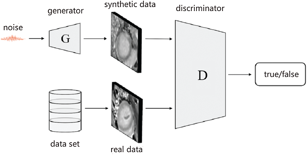
Figure 1: The structure of the GAN
The entire GAN training process is designed to find the balance between the generative network and the discriminative network. This makes the discriminator unable to judge whether the samples generated by the generator are real so that the generative network can achieve the optimal performance. This process can be expressed as formula (1):
The GAN generates new samples by fitting the original sample distribution. The new samples are generated from the distribution learned by the generative model, which makes it have new features that are different from the original samples. This characteristic makes it possible to use the samples generated by the generative network as new training samples to reach the goal of data expansion. The GAN has achieved good results in many computer vision fields. However, it has many problems in practical applications. It is very difficult to train a GAN. Once the data distribution and the distribution fitted by the generative network do not substantially overlap at the beginning of training, the gradient of the generative network can easily point to a random direction, which results in the problem of gradient disappearance [17]. The generator will try to generate a single sample that is relatively conservative but lacks diversity to make the discriminator give high scores which leads to the problem of mode collapse [18].
Many GAN variant models have been proposed to alleviate the situation of gradient disappearance and mode collapse. The more representative ones are deep convolutional GAN (DCGAN) [19], which combines a convolutional neural network with GAN, and conditional GAN [20] which adds a precondition control generator to the input data. The triple-GAN [21] adds a classifier based on the discriminator and generator, which can ensure that the classifier and generator achieve the optimal solution for classification from the perspective of game theory. In this approach, however, it is necessary to manually label samples. The improved Triple-GAN [22] method solves this problem and avoids the situation of gradient disappearance and training instability. In addition, the least squares GAN (LSGAN) [23] and wasserstein GAN (WGAN) [24] have made great improvements to the loss function. The WGAN uses wasserstein distance to measure the distribution distance, which makes the GAN training process more stable to a large extent. However, Gulrajan et al. [25] found that the WGAN uses a forced phase method to make the parameters of the network mostly focus on −0.01, 0.01, which wastes the fitting ability of the convolutional neural network. Therefore, they proposed the WGAN-GP model, which effectively alleviated this problem. Li et al. [26] introduced the gradient penalty term to the WGAN network to improve the convergence efficiency. The evolutionary GAN proposed by Wang et al. [27] is a variant model of a generative adversarial network that is based on evolutionary algorithms. It will perform mutation operations when the discriminator stops training to generate multiple generators as adversarial targets and uses a specific evaluation method to evaluate the quality and diversity of the generated images in different environments (the current discriminator). This series of operations can reserve one or more generators with better performance for the next round of training. This method that overcomes the limitations of a single adversarial target is able to keep the best offspring all the time. It effectively alleviates the problem of mode collapse and improves the quality of the generator.
Recently, many scholars have used GANs to augment training data samples. GANs have been used to augment the data of human faces and handwritten fonts [28]. Ali et al. [29] used the improved PGGAN to expand the skin injury dataset and increased the classification accuracy. Frid et al. [30] used a DCGAN and an ACGAN to expand the data of liver medical images and proved that the DCGAN has a greater improvement in the classification effect on this dataset. In contrast to affine transformation, a GAN can be used to generate images with new features by learning the real distribution.
The evolutionary GAN can improve the diversity and quality of generated samples. This study therefore uses an evolutionary GAN to perform data augmentation on cardiac magnetic resonance images. The main contributions of this study are as follows:
1. A cardiac magnetic resonance image data augmentation method based on an evolutionary GAN is proposed. This method generates high-quality and diverse samples to expand the training set and improves the value of various indicators of the classification results.
2. Linear interpolation of feature vectors is combined with the evolutionary GAN to synthesize new training samples and generate related linear interpolation labels. This not only expands the distribution of the entire training set, but also makes the discrete sample space continuous and improves the smoothness between domains, which better trains the model.
3. Various indicators of downstream classification tasks are used to optimize the model and the intensity of the experimental details.
The training process of the evolutionary GAN can be divided into three stages: mutation, evaluation, and selection. The first stage is mutation where the parent generator is mutated into multiple offspring generators; the second stage is evaluation where the adaptive score is worked out for each offspring generator of the current discriminator using an adaptive function; the third stage is selection where the offspring generator with the highest adaptive score is selected by sorting. The basic structure of the evolutionary GAN is shown in Fig. 2.
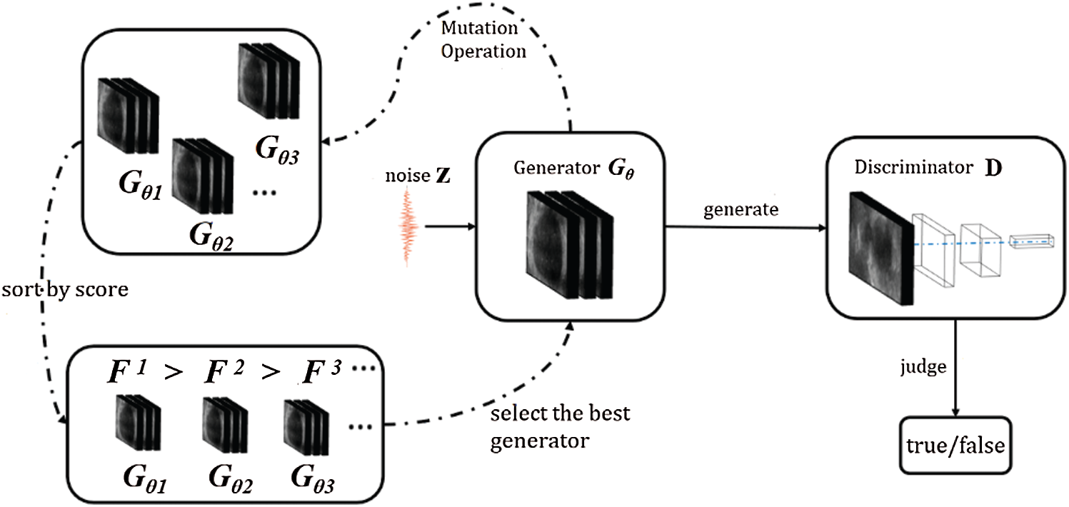
Figure 2: The structure of the evolutionary GAN
The evolutionary GAN uses different mutation methods to obtain offspring generators based on parent generators. These mutation operators are different training targets, the purpose of which is to reduce the distance between the generated distribution and the real data distribution from different angles. It should be noted that the best discriminator D* in formula (2) should be trained before each mutation operation.
Zhang et al. [31] proposed three mutation methods:
1) Maximum and minimum value mutation: Here the mutation has made little change to the original objective function, which provides an effective gradient and alleviates the situation of gradient disappearance. It can be written as formula (3):
2) Heuristic mutation: Heuristic mutation aims to maximize the log probability of the error of the discriminator. The heuristic mutation will not be saturated when the discriminator judges the generated sample as false and it still provides an effective gradient to get the generator continuously trained. It can be written as formula (4):
3) Least-squares mutation: Least-squares mutation can also avoid gradient disappearance. At the same time, compared with heuristic mutation, the least-square mutation does not generate false samples at a very high cost. It does not avoid punishment at a low cost, which can avoid mode collapse to a certain extent. It can be written as formula (5):
The evolutionary GAN uses the adaptive function to evaluate the performance of the generator and subsequently quantifies it as the corresponding adaptive score, which can be written as formula (6):
In this study, we describe the design of a data augmentation model for cardiac magnetic resonance medical images based on an evolutionary GAN. This approach can generate high-quality and diverse samples to expand the training set. The linear interpolation of related labels is generated by combining the linear interpolation of feature vector with the evolutionary GAN, which expands the distribution of the training set and makes the discrete sample space continuous to train the model better. The specific network structure is shown in Fig. 3:
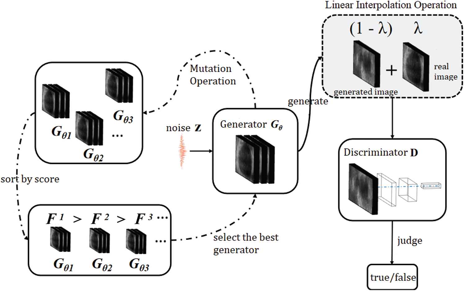
Figure 3: The proposed network
High quality and diversity of samples are needed when using a GAN for data augmentation. The evolutionary GAN is very suitable for data augmentation since it can be trained in a stable way and generates high-quality and diverse samples. The user can choose to focus on diversity or quality according to needs by adjusting the parameters in the adaptive function, which can make the process of data augmentation more operative. This study improves the evolutionary GAN and we name the improved model data augmentation evolutionary GAN (DAE GAN).
There is no difference in the input and output between the evolutionary GAN and vanilla GAN. The only exception is that after fixing the discriminator parameters multiple offspring generators are mutated based on the parent generator for training. The optimal one or more generators is selected as the parent generator in the next discriminator environment, after the evaluation by the adaptive function.
The evolutionary GAN greatly improves the diversity of generated samples. However, a certain number of training samples are required if we want to fully train the GAN model. In the case of too few training samples, the generator and discriminator are prone to reach the equilibrium point prematurely and also cause the problem of mode collapse in the generated data. This study uses the traditional affine transformation data augmentation methods before training the GAN to alleviate this problem, expanding the data by operations of horizontal flip, vertical inversion, translation, rotation, and others. The security of medical images was given careful consideration. We therefore did not add the original data with noise and avoided performing operations like cropping. In this way, we preserved the texture and edge features of the original data as far as possible. Traditional data augmentation only makes small changes to the original data and does not generate new features and the samples are also discrete. Thus, this study introduces linear interpolation.
Zhang et al. [31] proposed a data augmentation method that is irrelevant to the data described in their article. This method constructs virtual training samples from original samples, combines linear interpolation of feature vectors to synthesize new training samples, and generates related linear interpolation labels to expand the distribution of the entire training set. The specific formula is as follows (9):
The original input of the evolutionary GAN discriminator ought to be two samples after fixing the generator parameters: one is the generated sample (the discriminator tries to minimize the distance between the predicted label of this sample and “0”); the other is the real sample (the discriminator tries to minimize as much as possible the distance between the predicted label of this sample and “1”). The discriminator loss function of the original evolutionary GAN is described as follows in formula (10):
The expanded expression can be written as formula (11):
This study operates linear interpolation on the evolutionary GAN to modify the discriminator input from the original two pictures to one picture. The discriminator task is changed to minimize the distance between the predicted label of the fusion sample and ‘
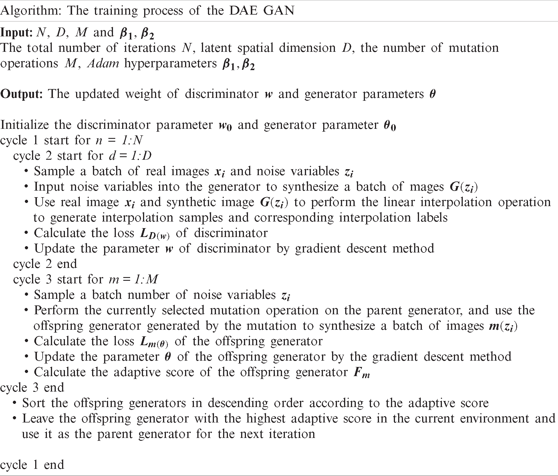
Typically, the GAN uses the noise
Table 1: The training process of the DAE GAN
4.1 Data Set and Preprocessing
The magnetic resonance data in this experiment were obtained from a partner hospital. All samples are two-dimensional short-axis primary T1 mapping images. The spatial distance of these cardiac magnetic resonance images ranges from 1.172 × 1.172 × 1.0 mm3 to 1.406 × 1.406 × 1.0 mm3 and the original pixel size is 256 × 218 × 1. The benign and malignant annotation and segmentation areas of these images are manually labeled and drawn by senior experts. The original image data is in the “.mha” for-mat. After a series of preprocessing operations, such as resampling, selection of regions of interest, normalization, and final selection of interest, we obtained a total of 298 images that consisted of 221 cardiomyopathy images and 77 non-diseased images. The size of the preprocessed image is 80 × 80 × 1. The preprocessed cardiac magnetic resonance image is shown in Fig. 4.
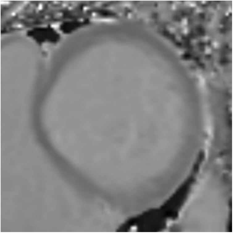
Figure 4: Cardiac magnetic resonance image region of interest
All samples were normalized in this experiment to ensure the consistency of training data. Weused affine transformations on the training set before training the GAN. This included horizontal flip, vertical flip, 90°, 180°, 270° rotation, 0°–20° random rotation and amplification, 0%–2% random rescaling of the vertical and horizontal axes, the small and specific amplitude of rotation and amplification, and translation and amplification. The goal of these steps was not to lose the original image information from the data. After augmenting the training set once, we performed two kinds of operations on the data: the first was to put it into the classifier for training directly, and to subsequently use the test set to get the classification results; the second was to put it into different GANs for training and generating new samples to train the classifier again.
The original evolutionary GAN uses the structure of a DCGAN. In this study, we use the residual structure shown in Fig. 5 in the generator and discriminator since the residual structure [33] can alleviate the gradient vanishing problem and accelerate the convergence rate. The goal is to train the high-performance generator more quickly in the same training time.
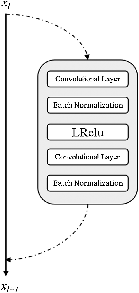
Figure 5: Residual block structure
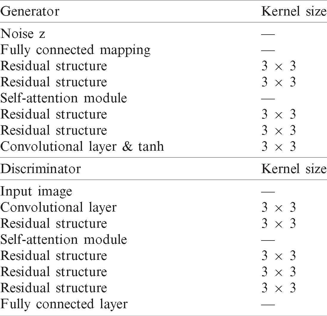
After adding the self-attention module [34], the detailed structure of the generator and discriminator and the output size of each layer is shown in Tab. 2.
Table 2: The structure of the DAE GAN
The DAE GAN experimental environment is as follows: Ubuntu 16.04.1 TLS, Tensorflow 1.14.0, two Nvidia Tesla M40 GPU with 12 GB video memory (used to train the generative models of diseased and non-diseased samples). The maximum storage capacity of the model is set to 4 to take into account the space occupation and accidental interruption.
4.3 The Generation Results of the DAE GAN
In this experiment, we use 5-fold cross-validation to dynamically divide the heart magnetic resonance image into a training set and a test set at a ratio of 0.8:0.2. We use only the training set in the DAE GAN training. Each model has been trained several times (≥ 5) in the experiment due to the uncertainty in the training process for the deep convolution model. The specific effect of the data augmentation method was verified by the average classification results.
The training set of the cardiac magnetic resonance image data is expanded after normalization and affine transformation. We train the DAE GAN model by following the steps of Algorithm 1. The effects of our approach on the samples generated in the training process of the generative model are shown in Fig. 6.
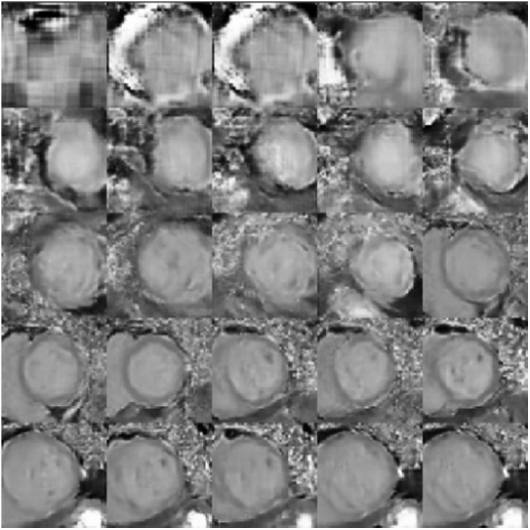
Figure 6: The changing process of the generated sample
A comparison of the samples generated by the trained generator versus the real samples is shown in Fig. 7.
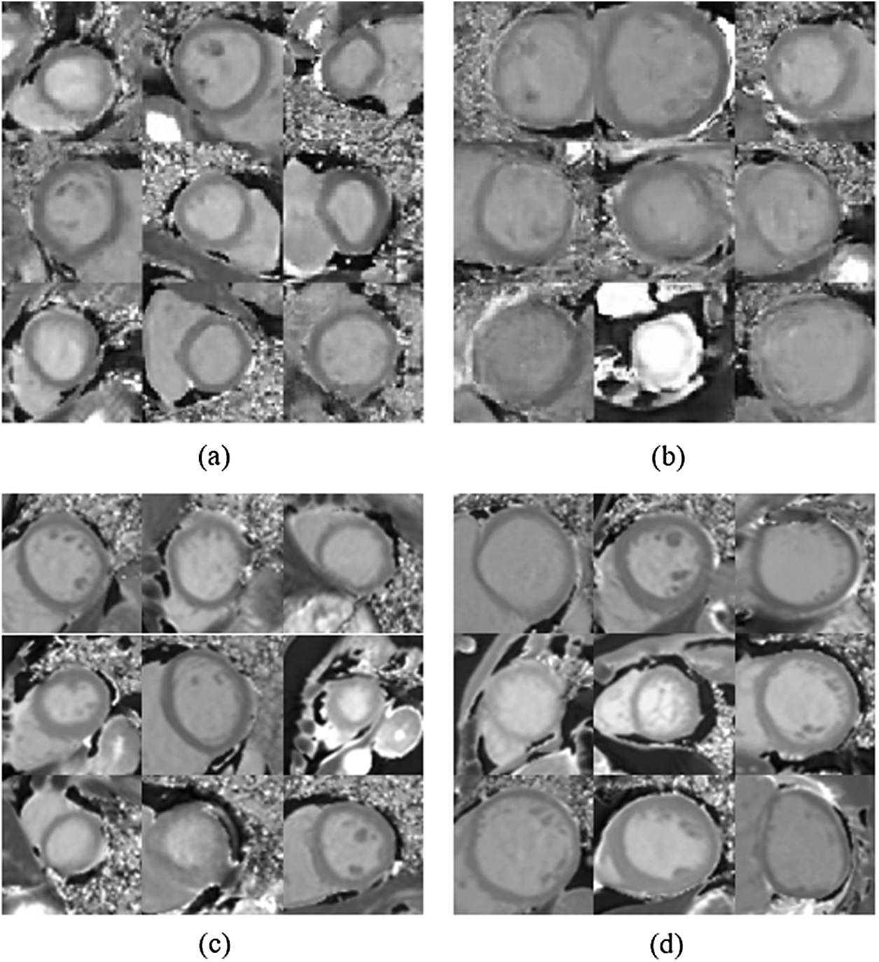
Figure 7: Comparison of generated samples with real samples. (a) Generated non-diseased samples (b) Generated non-diseased samples (c) Real non-diseased samples (d) Real diseased samples
4.4 Classification Experiment and Analysis of Experimental Results
The observation method has strong subjectivity. In this experiment, data augmentation is performed on small sample medical images. Consequently, the observation method can only be used as a reference evaluation standard. Our study uses the ResNet50 model and the Xception model [35] as a classifier to evaluate the effect of data augmentation. The classification results are used to uniformly evaluate the effects of various data augmentation methods.
In addition to the conventional accuracy index, we also calculate the two medical image classification indexes: sensitivity and specificity. These indicators are briefly explained here.
The accuracy rate is the probability that the diseased sample and the non-diseased sample are judged correctly. The calculation formula is described as follows in formula (13):
Sensitivity is the probability that a diseased sample is judged to be diseased. The calculation formula is described by formula (14):
Specificity is the probability of judging a non-diseased sample as non-diseased. The calculation formula is described as in formula (15):
TP stands for True Positive, which means that not only does the classifier judge it to be a diseased sample, but it is also a diseased sample. TN stands for True Negative. In this case, the classifier judges it to be a non-diseased sample, but it is in fact not a diseased sample. FP is short for False Positive, which means that the classifier judges it to be a diseased sample and it is a non-diseased sample. FN is short for False Negative. Here the classifier judges that the sample is not diseased but it is a diseased sample.
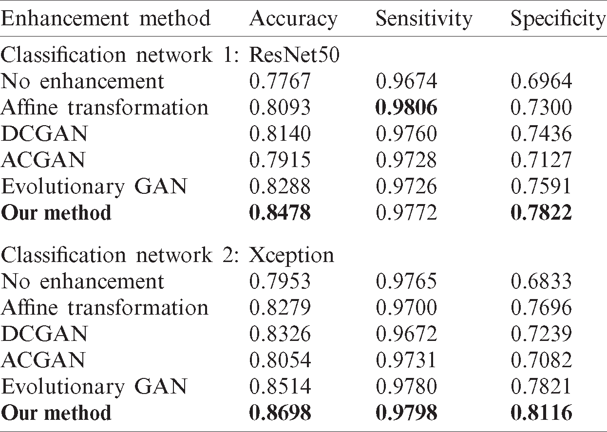
In this study, we use the Keras framework under the Ubuntu 16.04.1 TLS system environment for the classification experiment (version number 2.24). We use a Tesla M40 in the training process. The learning rate is set to 1e−4, and we use the RMSprop optimizer. We set the early stopping method to prevent overfitting and the fivefold cross-validation method is used to find the average classification result of the classifier. The average classification results of each augmentation method in the ResNet50 and Xception classification models are shown in Tab. 3.
Table 3: The classification results of enhancement methods
In the experiment, it is clear that the classification effect is not necessarily better as the number of generated samples increases. After adding a certain amount of data, the classification effect does not rise but decreases. At the same time, if only using generated samples without affine transformation data augmentation, the classification effect was not greatly improved compared with using affine transformation data augmentation alone. The specific experimental results are shown in Fig. 8.
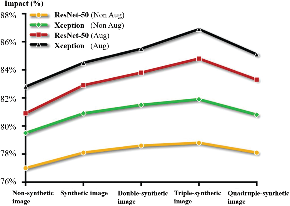
Figure 8: The impact of data volume on classification results
The experimental results show that we cannot completely obtain the original data distribution because the quality of the generated data remains poorer than the original data. The classification effect is slightly reduced by using only the generated data without the affine transformation data augmentation method. However, when the two methods are combined, the classification result of the classifier in-creases with the increase of the generated data and reaches the peak value when adding three times of the generated data. The addition of too much generated data leads to overfitting of the classification model and reduces the accuracy of classification.
Experiments were performed to compare the different models with the classification results without any data augmentation method. For the ResNet50 model, the classification accuracy increased from 0.7767 to 0.8478, the sensitivity increased from 0.9674 to 0.9772, and the specificity increased from 0.6964 to 0.7822. For the Xception model, the classification accuracy increased from 0.7953 to 0.8698, the sensitivity increased from 0.9765 to 0.9798, and the specificity increased from 0.6833 to 0.8116.
The DAE GAN model proposed in this paper can effectively expand the amount of cardiac magnetic resonance image data, alleviating the problem of the classification network not being fully trained due to the small amount of medical image data and uneven data. The classification accuracy of the DAE GAN in ResNet50 and Xception models was increased by 7.11% and 7.45%, respectively, compared with not using data augmentation methods. The method proposed in this paper increased the classification accuracy in ResNet50 and Xception by 3.85% and 4.19%, respectively, compared with affine trans-formation data augmentation, and the experimental results showed that the method is effective in different classification models.
Acknowledgement: We thank LetPub (www.letpub.com) for its linguistic assistance during the preparation of this manuscript.
Funding Statement: Y. F. received funding in part from the Sichuan Science and Technology Program (http://kjt.sc.gov.cn/) under Grant 2019ZDZX0005 and the Chinese Scholarship Council (https://www.csc.edu.cn/) under Grant 201908515022.
Conflicts of Interest: The authors declare that they have no conflicts of interest to report regarding the present study.
1. G. E. Hinton, N. Srivastava, A. Krizhevsky, I. Sutskever and R. R. Salakhutdinov. (2012). “Improving neural networks by preventing co-adaptation of feature detectors,” Computer Science, vol. 3, no. 4, pp. 212–223. [Google Scholar]
2. A. Renugambal and K. S. Bhuvaneswari. (2020). “Image segmentation of brain mr images using OTSU’s based hybrid WCMFO algorithm,” Computers, Materials & Continua, vol. 64, no. 2, pp. 681–700. [Google Scholar]
3. S. Geman, E. Bienenstock and R. Doursat. (1992). “Neural networks and the bias/variance dilemma,” Neural Computation, vol. 4, no. 1, pp. 1–58. [Google Scholar]
4. S. Ioffe and C. Szegedy. (2015). “Batch normalization: Accelerating deep network training by reducing internal covariate shift,” in Proc. ICML, Lille, France, pp. 448–456. [Google Scholar]
5. N. Srivastava, G. Hinton, A. Krizhevsky, I. Sutskever and R. R. Salakhutdinov. (2014). “Dropout: A simple way to prevent neural networks from overfitting,” Journal of Machine Learning Research, vol. 15, no. 1, pp. 1929–1958. [Google Scholar]
6. N. Morgan and H. Bourlard. (1990). “Generalization and parameter estimation in feedforward nets: Some experiments,” Advances in Neural Information Processing Systems, vol. 2, no. 1, pp. 630–637. [Google Scholar]
7. S. J. Nowlan and G. E. Hinton. (1992). “Simplifying neural networks by soft weight-sharing,” Neural Computation, vol. 4, no. 4, pp. 473–493. [Google Scholar]
8. A. Krogh and J. A. Hertz. (1991). “A simple weight decay can improve generalization,” in Proc. NIPS, Denver, Colorado, USA, pp. 950–957. [Google Scholar]
9. A. Krizhevsky, I. Sutskever and G. E. Hinton. (2012). “Imagenet classification with deep convolutional neural networks,” in Proc. NIPS, Red Hook, NY, USA, pp. 1097–1105. [Google Scholar]
10. H. R. Roth, L. Lu, J. Liu, J. Yao, A. Seff et al. (2016). , “Improving computer-aided detection using convolutional neural networks and random view aggregation,” IEEE Transactions on Medical Imaging, vol. 35, no. 5, pp. 1170–1181. [Google Scholar]
11. A. A. A. Setio, F. Ciompi, G. Litjens, P. Gerke, C. Jacobs et al. (2016). , “Pulmonary nodule detection in CT images: False positive reduction using multi-view convolutional networks,” IEEE Transactions on Medical Imaging, vol. 35, no. 5, pp. 1160–1169. [Google Scholar]
12. D. V. Sang, L. T. B. Cuong and D. P. Thuan. (2017). “Facial smile detection using convolutional neural networks,” in Proc. KSE, Hue, Vietnam, pp. 136–141. [Google Scholar]
13. H. C. Shin, N. A. Tenenholtz, J. K. Rogers, C. G. Schwarz, M. L. Senjem et al. (2018). , “Medical image synthesis for data augmentation and anonymization using generative adversarial networks,” in Simulation and Synthesis in Medical Imaging, 1\textrm{st} ed., vol. 11037. Cham, USA: Springer International Publishing, pp. 1–11. [Google Scholar]
14. J. Liu, W. Wang, J. Chen, G. Sun and A. Yang. (2019). “Classification and research of skin lesions based on machine learning,” Computers, Materials & Continua, vol. 61, no. 3, pp. 1187–1200. [Google Scholar]
15. L. Pan, J. Qin, H. Chen, X. Xiang, C. Li et al. (2019). , “Image augmentation-based food recognition with convolutional neural networks,” Computers, Materials & Continua, vol. 59, no. 1, pp. 297–313. [Google Scholar]
16. I. J. Goodfellow, J. Pouget-Abadie, M. Mirza, B. Xu, D. Warde-Farley et al. (2014). , “Generative adversarial networks,” Advances in Neural Information Processing Systems, vol. 27, pp. 2672–2680. [Google Scholar]
17. M. Arjovsky and L. Bottou. (2017). “Towards principled methods for training generative adversarial networks,” in Proc. ICRL, Toulon, France, pp. 1050–1066. [Google Scholar]
18. D. Bang and H. Shim. (2018). “MGGAN: Solving mode collapse using manifold guided training,” in Proc. CVPR, Salt Lake City, UT, USA, pp. 177–192. [Google Scholar]
19. A. Radford, L. Metz and S. Chintala. (2015). “Unsupervised representation learning with deep convolutional generative adversarial networks,” in Proc. ICLR, San Diego, CA, USA, pp. 232–247. [Google Scholar]
20. M. Mirza and S. Osindero. (2014). “Conditional generative adversarial nets,” in Proc. CVPR, Columbus, Ohio, USA, pp. 1710–1716. [Google Scholar]
21. C. Li, K. Xu, J. Zhu and B. Zhang. (2017). “Triple generative adversarial nets,” in Proc. NIPS, Long Beach, CA, USA, pp. 4088–4098. [Google Scholar]
22. K. Fang and J. Q. OuYang. (2020). “Classification algorithm optimization based on Triple-GAN,” Journal on Artificial Intelligence, vol. 2, no. 1, pp. 1–15. [Google Scholar]
23. X. Mao, Q. Li, H. Xie, R. Y. K. Lau, Z. Wang et al. (2017). , “Least squares generative adversarial networks,” in Proc. ICCV, D. C., USA, pp. 2813–2821. [Google Scholar]
24. M. Arjovsky, S. Chintala and L. Bottou. (2017). “Wasserstein gan,” in Proc. ICML, Sydney, NSW, Australia, pp. 654–685. [Google Scholar]
25. I. Gulrajani, F. Ahmed, M. Arjovsky, V. Dumoulin and A. Courville. (2017). “Improved training of wasserstein gans,” in Proc. NIPS, Long Beach, CA, USA, pp. 5767–5777. [Google Scholar]
26. X. Li, C. Ye, Y. Yan and Z. Du. (2019). “Low-dose ct image denoising based on improved WGAN-GP,” Journal of New Media, vol. 1, no. 2, pp. 75–85. [Google Scholar]
27. C. Wang, C. Xu, X. Yao and D. Tao. (2019). “Evolutionary generative adversarial networks,” IEEE Transactions on Evolutionary Computation, vol. 23, no. 6, pp. 921–934. [Google Scholar]
28. A. Antoniou, A. Storkey and H. Edwards. (2017). “Data augmentation generative adversarial networks,” in Proc. CVPR, Honolulu, HI, USA, pp. 2116–2129. [Google Scholar]
29. I. S. Ali, M. F. Mohamed and Y. B. Mahdya. (2020). “Data augmentation for skin lesion using self-attention based progressive generative adversarial network,” Expert Systems with Applications, vol. 165, pp. 113922. [Google Scholar]
30. M. Frid-Adar, I. Diamant, E. Klang, M. Amitai, J. Goldberger et al. (2018). , “GAN-based synthetic medical image augmentation for increased CNN performance in liver lesion classification,” Neurocomputing, vol. 321, no. 5, pp. 321–331. [Google Scholar]
31. H. Zhang, M. Cisse, Y. N. Dauphin and D. L. Paz. (2018). “Mixup: Beyond empirical risk minimization,” in Proc. ICLR, Vancouver, BC, Canada, pp. 1760–1772. [Google Scholar]
32. Y. M. Ben and D. Weinshall. (2018). “Gaussian mixture generative adversarial networks for diverse datasets, and the unsupervised clustering of images,” Computing Research Repository, vol. 1808, pp. 10356. [Google Scholar]
33. K. He, X. Zhang, S. Ren and J. Sun. (2016). “Deep residual learning for image recognition,” in Proc. CVPR, Las Vegas, NV, USA, pp. 770–778. [Google Scholar]
34. Z. Han, G. Ian, D. Metaxas and O. Augustus. (2018). “Self-attention generative adversarial networks,” in Proc. ICLR, Vancouver, BC, Canada, pp. 7354–7363. [Google Scholar]
35. F. Chollet. (2017). “Xception: Deep learning with depthwise separable convolutions,” in Proc. CVPR, Honolulu, HI, USA, pp. 1251–1258. [Google Scholar]
 | This work is licensed under a Creative Commons Attribution 4.0 International License, which permits unrestricted use, distribution, and reproduction in any medium, provided the original work is properly cited. |