Computers, Materials & Continua DOI:10.32604/cmc.2021.016108
Article

An Enhanced Jacobi Precoder for Downlink Massive MIMO Systems

Park Chan-Yeob, Hyun-Ro Jae, Jun-Yong Jang and Song Hyoung-Kyu*

Department of Information and Communication Engineering, and Convergence Engineering for Intelligent Drone, Sejong University, Seoul, 05006, Korea
*Corresponding Author: Song Hyoung-Kyu. Email: songhk@sejong.ac.kr
Received: 23 December 2020; Accepted: 26 January 2021

Abstract: Linear precoding methods such as zero-forcing (ZF) are near optimal for downlink massive multi-user multiple input multiple output (MIMO) systems due to their asymptotic channel property. However, as the number of users increases, the computational complexity of obtaining the inverse matrix of the gram matrix increases. For solving the computational complexity problem, this paper proposes an improved Jacobi (JC)-based precoder to improve error performance of the conventional JC in the downlink massive MIMO systems. The conventional JC was studied for solving the high computational complexity of the ZF algorithm and was able to achieve parallel implementation. However, the conventional JC has poor error performance when the number of users increases, which means that the diagonal dominance component of the gram matrix is reduced. In this paper, the preconditioning method is proposed to improve the error performance. Before executing the JC, the condition number of the linear equation and spectrum radius of the iteration matrix are reduced by multiplying the preconditioning matrix of the linear equation. To further reduce the condition number of the linear equation, this paper proposes a polynomial expansion precondition matrix that supplements diagonal components. The results show that the proposed method provides better performance than other iterative methods and has similar performance to the ZF.

Keywords: Jacobi (JC); massive MIMO; precondition; polynomial expansion; linear precoding

1  Introduction

MIMO technology has been widely used in wireless communication. The emerging technology among MIMO systems is massive MIMO, which uses hundreds of antennas in a base station (BS) and transmits data to many users. Because a large number of antennas is used in a BS, massive MIMO systems have greater spectral efficiency than conventional ones. For multi-user data transmission in downlink systems, a BS performs precoding in advance to eliminate inter-user interference. The ZF is the optimal method in the downlink massive MIMO systems since the channel property has asymptotic orthogonality [1–5]. However, the computational complexity of ZF is O(K3) when calculating the inversion of the gram matrix, where K is the total number of users [6–8]. Therefore, huge computational complexity is required to provide services to many users. To solve the problem, several low-complexity methods were proposed in [9–19]. Approximate inverse matrix methods with low complexity using Neumann series expansion (NSE) were proposed [9,10]. The NSE are used to approximate the inverse matrix, though when the numbers of BS antennas and users are small, they suffer from performance degradation. Moreover, their computational complexity increases to O(K3) to achieve reasonable error performance. Another type of low-complexity methods is based on iterative approximate linear equations; examples include the Gauss–Seidel (GS), the successive over relaxation (SOR), the symmetric SOR (SSOR), the Richardson (RI), and the JC method. It has been proved that the convergence rate of the GS, the SOR, and the SSOR is faster than that of the NSE’s [11–13]. However, parallel implementation for GS, SOR, and SSOR is very difficult because of the inner product in forward substitution that is used to take advantage of the lower matrix, whereas, the RI and the JC can be implemented in parallel [14,15]. The JC includes a simple approximate linear equation and achieves near optimal performance when the ratio α is large, where α is defined as NtK, and Nt is the number of BS antennas. Otherwise, when α is small, the JC provides poor error performance. The RI can achieve optimal performance irrespective of the size of the channel matrix, but its convergence rate becomes smaller as the number of users increases. For improved performance of the JC precoder, the author in [16] proposed a joint conjugate gradient and Jacobi (CJ) method-based precoding. The author in [17] proposed a detector based on joint steepest descent and Jacobi (SJ) method in the uplink massive MIMO systems. The CJ and the SJ have complex division operations that are not hardware-friendly [14]. The author in [18] proposed the Damped Jacobi (DJ) method, which achieves relatively good performance, even with an increase in the number of users. However, the performance of DJ converges toward an error floor quickly as the number of users is increased. Hence, the DJ has limitations in performance in the environments with many users.

To solve the above problem and improve performance, this paper proposes a precondition Jacobi (PJC)-based precoder. The convergence rate is increased due to the use of precondition matrix multiplication, which is performed in each iteration., and as such allowing fast convergence. To accelerate convergence and obtain accurate solutions, the precondition matrix should satisfy three conditions. First, it should be an accurate approximate inverse matrix of the gram matrix. Second, the equation requires reasonable computational complexity to create it. Third, the total iterative equation should be solved easily with it. This paper proposes a polynomial expansion using the RI to obtain the precondition matrix. Moreover, it proposes a modified iteration equation to reduce the computational complexity by avoiding matrix–matrix multiplication.

The remainder of this paper is organized as follows. Section 2 presents the model for downlink massive MIMO systems. Section 3 explains the conventional JC. In Section 4, the PJC is proposed and compared with other iterative methods in regard to computational complexity. Section 5 provides convergence rate and simulation results. Lastly, Section 6 presents a conclusion.

2  Massive MIMO System Model

This paper considers the downlink massive MIMO system. The number of BS antennas is Nt, and the total number of users with a single antenna is K. The downlink massive MIMO system model is shown in Fig. 1. The channel matrix between the number of BS antennas and the number of total users is as follows:

H=[h1h2,…,hK]T,(1)

where hij is the i -th element of hi(i=1,2,…,K) and has an independent and identically distributed (i.i.d) complex baseband Rayleigh flat fading channel coefficient. When Z=[z1,z2,…,zK] is the precoding matrix, the i -th received symbol yi is as follows:

yi=PhiTzi||Z||Fxi+∑t=1,t≠iKPhtTzt||Z||Fxt+ni,(2)

where P is the transmit power, zi is the i -th vector of Z, xi is the complex transmit symbol with zero mean and unit variance, ni is the i -th complex additive white Gaussian noise (AWGN) with zero mean and unit variance, and ||⋅||F is the Frobenius norm.

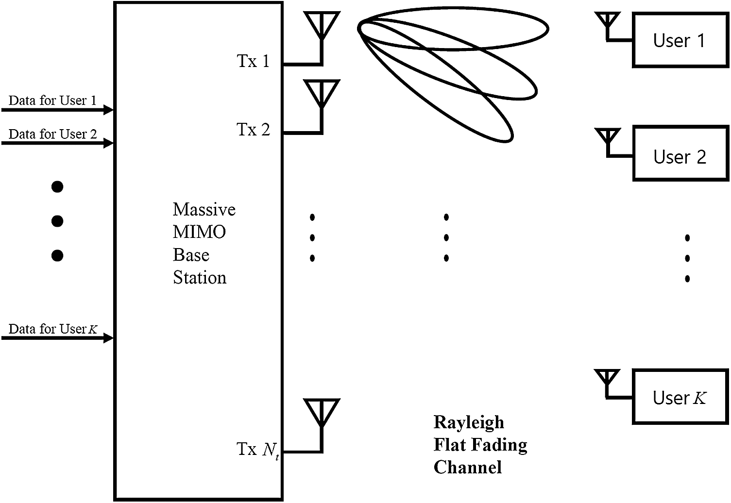
Figure 1: The downlink massive MIMO system model

3  Conventional JC Precoding

This paper uses the JC to avoid the direct inversion of gram matrix W=HHH. To solve the linear equation of Ws=x, the iterative method expresses the following:

Ms(n)=Ns(n-1)+x,s(n)=Bs(n-1)+c,(3)

where M and N are decomposed from W, W=M-N, B and c are expressed as B=M-1N and c=M-1x. n is the number of iterations. The iterative method depends on M and N. In the JC, M and N are chosen as follows:

M=DN=-(L+U),(4)

where D is the diagonal matrix of W, L is the strict lower matrix of W, and Uis the strict upper matrix of W. The n -th iterative solution of the JC is as follows:

s(n)=D-1(x-(L+U)s(n-1)),(5)

where x is a K×1 modulated vector. s(0) is an initial solution and is generally used as follows:

s(0)=D-1x.(6)

After the final iteration, the transmit symbol vector s is multiplied by a matched filter and normalization factor as follows:

s=1βHHs(n),(7)

where β is the normalization factor that prevents variations in transmit power.

4  Proposed JC Method

In this section, the proposed precondition matrix in the JC is explained. It aims to improve the bit error rate (BER) performance of the downlink massive MIMO systems. Research related to the JC such as the CJ, the SJ and the DJ has been studied. However, the CJ and the SJ have complex division processes, which are the most expensive operations. Additionally, the DJ provides low error performance in an environment with a large number of users since the convergence rate is low and the condition number of the linear equation is high.

In order to solve the above problem, this paper proposes the PJC. It has two steps. First, the precondition matrix is computed by the simplest polynomial expansion up to the first-order term. When it exceeds the second-order term, the computational complexity is O(K3) because of matrix–matrix multiplication. The diagonal component is introduced in the second-order term to improve performance. After the precondition matrix is calculated, both sides of the linear equation are multiplied with the precondition matrix to reduce the condition number of the linear equation. The condition number of the linear equation measures the sensitivity of the solution to small changes in the input. Thus, when the linear equation has a low condition number, the situation is well conditioned [20]. Second, the JC is performed with a precondition matrix to reduce the spectrum radius of the iterative method. However, if it is performed by simply applying the precondition matrix, matrix–matrix multiplication is performed and the computational complexity is O(K3). In order to reduce the computational complexity, only the necessary matrix components are calculated, and the iteration equation is transformed into a matrix–vector multiplication.

4.1 Proposed Precondition Matrix

The preconditioning process reduces the condition number of the linear equation. The convergence rate is increased as the condition number of the linear equation is decreased [20]. To reduce the condition number of the linear equation, the precondition matrix is computed by polynomial expansion. The equation of polynomial expansion is as follows:

W-1≈∑i=0∞(M-1N)iM-1.(8)

In order to converge into the inverse matrix, the matrix M and N should be properly selected. The decomposed matrix is selected by the RI. The convergence rate of the RI is faster than that of the JC and is more suitable for environments with many users whereas the performance of the JC is affected by the diagonal dominant components of W [21]. In the RI, M is 1ωI, and N is 1ωI-W. Therefore, the precondition matrix P formed by polynomial expansion when applying the RI is as follows:

P=(I+(I-ωW)+(I-ωD)2)ω,(9)

where ω is the relaxation parameter, which is originally expressed as an eigenvalue of the gram matrix. Due to the computational complexity, ω is estimated as 1Nt+K [14]. In order to approximate the inverse matrix of W accurately, the second-order term is used. The diagonal components of the gram matrix have a high proportion in the massive MIMO environment. Thus, the diagonal components are introduced. After the precondition matrix is computed, it is multiplied by both sides of the linear equation:

PWs¯=Px.(10)

The preconditioning process accelerates the convergence rate as the condition number of PW is decreased. The condition number of the precondition matrix with the second-order term is lower than that with the first-order term since it is slightly more similar to the inverse matrix of W thanks to the introduction of the diagonal components. Since the expression in (10) calculates the matrix–matrix multiplication, the computational complexity of PJC exceeds O(K3). To reduce the computational complexity, the proposed equation is transformed in the next section to calculate only the necessary components.

4.2 Proposed JC Method with Precondition Matrix

In order to accelerate the convergence of the iterative method, the precondition matrix is applied to the JC. The linear equation multiplied by the precondition matrix is as follows:

W¯s¯=x¯,(11)

where W¯=PW,and Px=x¯. The computational complexity here is O(K3). However, the computational complexity of the PJC is reduced to O(K2) by multiplying only the necessary elements. In the JC, W¯ is decomposed as follows:

W¯=D¯+L¯+U¯,(12)

where D¯ is the diagonal matrix of W¯, L¯ is the strict lower matrix of W¯, and U¯ is the strict upper matrix of W¯. The PJC with the precondition matrix is as follows:

s¯(n)=D¯-1[x¯-(L¯+U¯)s¯(n-1)],n=1,2,….(13)

However, (10) should calculate the upper and lower triangular components of W¯. The computational complexity for calculating L¯ and U¯ is O(K3). Therefore, this paper propose a modified equation that does not need to find the components of L¯ and U¯ to make the computational complexity O(K2). The modified equation is as follows:

s¯(n+1)=D¯−1(x¯−(W¯−D¯)s¯(n))=s¯(n)+D¯−1(Px−PWs¯(n))=s¯(n)+D¯−1P(x−Ws¯(n))n=1,2,…,(14)

where s¯(0) is an initial value. In the PJC, s¯(0) is expressed as follows:

s¯(0)=D¯-1x¯.(15)

Consequently, the proposed algorithm for designing PJC precoders is summarized as follows:

Step 1: Input parameter x, H, n, β=KNt-K [11], ω

Step 2: Initialization

P=(2ωI-ω2W)+(I-wD)2ω

Step 3: Calculate the diagonal component of

for u=1:1:KD¯u,u=∑v=1KPu,vWv,uendx¯=Pxs(0)=D¯-1x¯

Step 4: Calculate JC precoder

fork=1:1:ns(k)=s(k-1)+D¯-1P(x-Ws(k-1))end

Step 4: ZF precoding

s=1βHHs(n)

4.3 Computational Complexity Analysis

The computational complexity is an important indicator for evaluating the performance of an iterative method. This paper defines the computational complexity as the required number of multiplications. Tab. 1 shows the computational complexity of the PJC and several conventional methods. It is more than twice that of the RI, the JC, and the DJ since the computational complexity O(K2) is required to calculate the precondition matrix. However, the performance of the PJC is higher than that of the RI, the JC, and the DJ thanks to the use of the precondition matrix.

Table 1: The computational complexity of the PJC, the RI, the JC, the DJ, and the ZF

5  Performance Evaluation

5.1 Convergence Rate Analysis

The convergence rates of different iteration methods can be compared by calculating the spectral radius corresponding to each iteration matrix as well as the condition numbers of linear equations. The condition number of linear equation is obtained by calculating the largest singular value of a linear equation. To reduce the condition number of a linear equation, the precondition matrix similar to the inverse matrix of W should be multiplied in both sides of the linear equation. In Section 4, the precondition matrix that approximates the inverse matrix of W using polynomial expansion and introducing the diagonal components of W is proposed.

Fig. 2 shows the condition number of W¯ when the precondition matrix is multiplied. It consisted of the first-order term of polynomial expansion or the second-order term of diagonal components. The convergence rate of the iterative method is increased as the condition number of W¯ is decreased. The condition number of the linear equation is calculated as follows:

κ(W¯)=∥W¯∥∥W¯-1∥.(16)

It is shown that the condition number of the precondition matrix with the second-order term is lower than that with the first-order term because the precondition matrix is slightly more similar to the inverse matrix of W thanks to introducing the diagonal components.

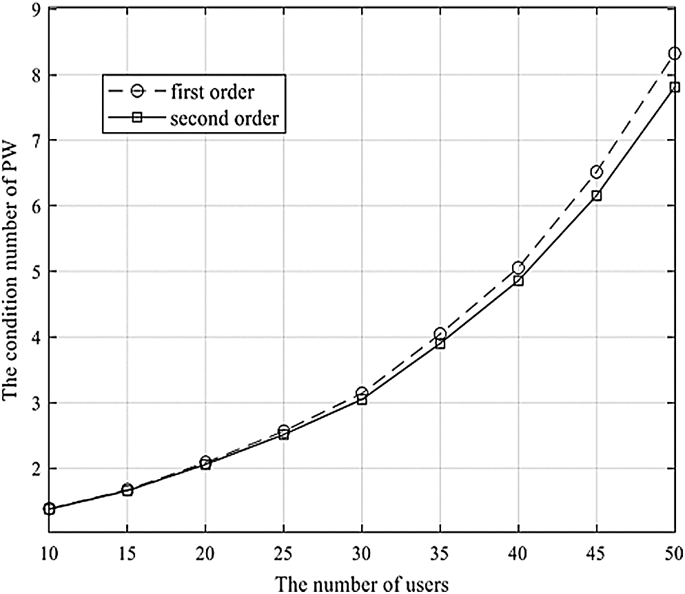
Figure 2: The condition numbers of linear equations, multiplied by the precondition matrix when Nt = 100

To evaluate the convergence rate, the iterative method equation is expressed as s(n)=Bs(n-1)+c, where B is iteration matrix. The spectral radius of the iterative method is measured as the largest eigenvalue of B. It should be smaller than 1 to converge into an accurate solution of the linear equation. The convergence rate is increased as the spectrum radius is decreased. Fig. 3 compares the spectrum radii of several iterative methods. Each compared iterative matrix is as follows:

BJC=(I-D-1W)2BRI=(I-ωW)2BDJ=(I-ω¯D-1W)2BPJC=(I-D¯-1W¯).(17)

In order to have similar computational complexity with the PJC, the iterative matrix of the RI, the DJ, and the PJC is squared. Generally, when α is large, the diagonal dominant components of W are increased due to the law of large numbers, and the effect of small-scale fading and thermal noise can be averaged out [22]. The performance of the iterative method is improved as the number of diagonally dominant components of W is increased. In [10], the authors proved that W is fully diagonal dominant when α is larger than 5.83. The JC cannot converge when the diagonal dominance of W is small. Furthermore, Fig. 3 shows that the JC cannot converge when the number of users is higher than 25. In contrast, the RI and DJ can converge when α is smaller than 5.83. However, the spectrum radius of the PJC is lower than 1 for any α and is also lower than spectrum radii of the RI and the DJ. The computational complexity of the PJC is higher than those of the JC, the RI, and the DJ due to multiplying the precondition matrix. However, it can be reduced to O(K2) from O(K2) despite the increase of computational complexity.

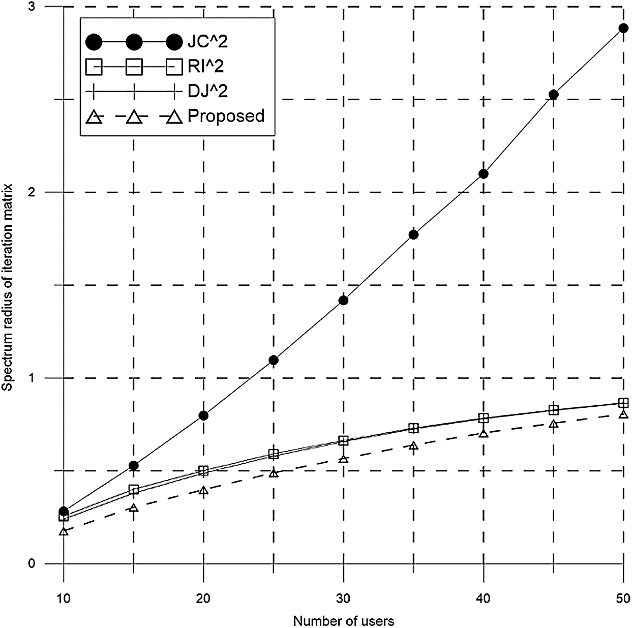
Figure 3: Spectrum radii of iteration matrices of several iterative methods when Nt = 100

5.2 Simulation Results

This paper uses ZF as an optimal precoder. In MU MIMO systems, the minimum mean square error (MMSE) precoder provides better error performance than the ZF precoder. However, in the massive MIMO systems, the ZF precoder shows the same error performance as the MMSE precoder. In order to evaluate performance, the BER performances are measured. In all simulations, the number of BS antennas is fixed at 100 for the downlink massive MIMO systems. The downlink channel is modeled by the Rayleigh flat fading channel. Moreover, it is assumed that the BS knows perfect channel state information (CSI) for all users.

Fig. 4 shows the BER performances for the RI, the PJC, and the ZF precoding methods in quadrature phase shift keying (QPSK). Since the number of diagonally dominant components of W are decreased by decreasing α, the JC provides poor error performance. Furthermore, the SJ and the CJ find the initial value with the conjugate gradient and steepest descent algorithms, which enable them to accelerate convergence. After the SJ and the CJ calculate the initial value, the JC is performed. Therefore, these perform similar to the JC in the environment with many users. As shown in Fig. 4a, the performances of the PJC and the RI are increased as the number of iterations is increased since α is large. Meanwhile, as illustrated in Fig. 4b, although the number of iterations is increased, the improvement in performance for the RI is lower than that for the PJC. Furthermore, the performance of the RI is not increased below 10−5 even though the number of iterations is increased. Lastly, in Fig. 4c we can observe that the PJC shows a significant improvement in performance, while the RI has little improvement in performance. The performance of the RI converges toward an error floor. Moreover, the performance of the PJC continues to increase as the number of iterations increases. In conclusion, Fig. 4 shows that the difference in performance between the PJC and the RI is increased as the number of users is increased. In other words, the PJC is more efficient than the RI in environments with a large number of users.

Figure 4: BER performance comparison of RI, PJC, and ZF precoding methods in QPSK(a) Nt = 100, K = 30 (b) Nt = 100, K = 40 (c) Nt = 100, K = 50

Fig. 5 shows the BER performances for the DJ, the PJC, and the ZF precoding methods in 16 quadrature amplitude modulation (QAM). Generally, the results presented in Fig. 5 are similar to those in Fig. 4. It can observed that the JC suffers from low reliability. In Fig. 5a, the performances of the PJC and the DJ are increased as the number of iterations is increased. Since α is large, there is influence from the diagonally dominant component, and the PJC and DJ shows almost the same BER performance. In Fig. 5b, the performance of the DJ is lower than that of the PJC in all iterations. Furthermore, in Fig. 5c, it gradually converges toward an error floor at 18 dB even though the number of iterations is increased. Therefore, it is not increased below 10−4 even though the number of iterations is increased. In contrast, the performance of the PJC continues to increase as the number of iterations is increased.

Figure 5: BER performance comparison of the DJ, the PJC, and the ZF precoding methods in 16QAM(a) Nt = 100, K = 30 (b) Nt = 100, K = 40 (c) Nt = 100, K = 50

The PJC obtains these promising results since the precondition matrix is multiplied with the linear equation to reduce the condition number of the linear equation and the spectral radius of the iterative matrix. Overall, it performs better than the RI and the DJ for the BER performance in environments with many users.

6  Conclusion

The iterative method is one solution to solve the computational complexity problem in the massive MIMO systems. This paper proposes an improved the JC-based precoder in the massive MIMO systems with a large number of users. The error performance is improved by using the precondition matrix. In order to accelerate convergence, the precondition matrix is multiplied with the linear equation. Then, the PJC is transformed to avoid matrix–matrix multiplication. None of the elements of the matrix that are multiplied with the precondition matrix and the gram matrix are required. Although the computational complexity of the PJC is increased compared to traditional methods, it overcomes the poor performance of the conventional JC when α is small. Furthermore, the PJC provides better BER performance improvements than the JC, the RI, and the DJ with similar computational complexity.

Funding Statement: This research was supported by the MSIT (Ministry of Science and ICT), Korea, under the ITRC (Information Technology Research Center) support program (IITP-2019-2018-0-01423) supervised by the IITP (Institute for Information & communications Technology Promotion), and supported by the Basic Science Research Program through the National Research Foundation of Korea (NRF) funded by the Ministry of Education (2020R1A6A1A03038540).

Conflicts of Interest: The authors declare that they have no conflicts of interest to report regarding the present study.

References

 1.  F. Rusek, D. Persson, B. K. Lau, E. G. Larsson, T. L. Marzetta et al. (2013). , “Scaling up MIMO: Opportunities and challenges with very large arrays,” IEEE Signal Processing Magazine, vol. 30, no. 1, pp. 40–60. [Google Scholar]

 2.  E. G. Larsson, O. Edfors, F. Tufvesson and T. L. Marzetta. (2014). “Massive MIMO for next generation wireless systems,” IEEE Communications Magazine, vol. 52, no. 2, pp. 186–195. [Google Scholar]

 3.  L. Lu, G. Y. Li, A. L. Swindlehurst, A. Ashikhmin and R. Zhang. (2014). “An overview of massive MIMO: Benefits and challenges,” IEEE Journal of Selected Topics in Signal Processing, vol. 8, no. 5, pp. 742–758. [Google Scholar]

 4.  T. L. Marzetta. (2015). “Massive MIMO: An introduction,” Bell Labs Technical Journal, vol. 20, pp. 11–22. [Google Scholar]

 5.  E. Björnson, E. G. Larsson and T. L. Marzetta. (2016). “Massive MIMO: Ten myths and one critical question,” IEEE Communications Magazine, vol. 54, no. 2, pp. 114–123. [Google Scholar]

 6.  M. A. Albreem, M. Juntti and S. Shahabuddin. (2019). “Massive MIMO detection techniques: A survey,” IEEE Communications Surveys & Tutorials, vol. 21, no. 4, pp. 3109–3132. [Google Scholar]

 7.  Z. Zhang, J. Wu, X. Mal, Y. Dong, Y. Wang et al. (2016). , “Reviews of recent progress on low-complexity linear detection via iterative algorithms for massive MIMO systems,” in 2016 IEEE/CIC Int. Conf. on Communications in China (ICCC WorkshopsChengdu, pp. 1–6. [Google Scholar]

 8.  N. Fatema, G. Hua, Y. Xiang, D. Peng and I. Natgunanathan. (2018). “Massive MIMO linear precoding: A survey,” IEEE Systems Journal, vol. 12, no. 4, pp. 3920–3931. [Google Scholar]

 9.  O. Gustafsson, E. Bertilsson, J. Klasson and C. Ingemarsson. (2017). “Approximate Neumann series or exact matrix inversion for massive MIMO?,” in 2017 IEEE 24th Symp. on Computer Arithmetic (ARITHLondon, pp. 62–63. [Google Scholar]

10. D. Zhu, B. Li and P. Liang. (2015). “On the matrix inversion approximation based on Neumann series in massive MIMO systems,” in 2015 IEEE Int. Conf. on Communications (ICCLondon, pp. 1763–1769. [Google Scholar]

11. X. Gao, L. Dai, J. Zhang, S. Han and I. Chih-Lin. (2015). “Capacity-approaching linear precoding with low-complexity for large-scale MIMO systems,” in 2015 IEEE Int. Conf. on Communications (ICCLondon, pp. 1577–1582. [Google Scholar]

12. X. Gao, L. Dai, Y. Hu, Z. Wang and Z. Wang. (2014). “Matrix inversion-less signal detection using SOR method for uplink large-scale MIMO systems,” in 2014 IEEE Global Communications Conf., Austin, TX, pp. 3291–3295. [Google Scholar]

13. T. Xie, L. Dai, X. Gao, X. Dai and Y. Zhao. (2016). “Low-complexity SSOR-based precoding for massive MIMO systems,” IEEE Communications Letters, vol. 20, no. 4, pp. 744–747. [Google Scholar]

14. B. Kang, J. Yoon and J. Park. (2017). “Low-complexity massive MIMO detectors based on Richardson method,” Etri Journal, vol. 39, no. 3, pp. 326–335. [Google Scholar]

15. Y. Lee. (2017). “Decision-aided Jacobi iteration for signal detection in massive MIMO systems,” Electronics Letters, vol. 53, no. 23, pp. 1552–1554. [Google Scholar]

16. W. Song, X. Chen, L. Wang and X. Lu. (2016). “Joint conjugate gradient and Jacobi iteration based low complexity precoding for massive MIMO systems,” in 2016 IEEE/CIC Int. Conf. on Communications in China (ICCCChengdu, pp. 1–5. [Google Scholar]

17. X. Qin, Z. Yan and G. He. (2016). “A near-optimal detection scheme based on joint steepest descent and Jacobi method for uplink massive MIMO systems,” IEEE Communications Letters, vol. 20, no. 2, pp. 276–279. [Google Scholar]

18. Y. Zhang, A. Yu, X. Tan, Z. Zhang, X. You et al. (2018). , “Adaptive damped Jacobi detector and architecture for massive MIMO uplink,” in 2018 IEEE Asia Pacific Conf. on Circuits and Systems (APCCASChengdu, pp. 203–206. [Google Scholar]

19. J. Ro, W. Lee, J. Ha and H. Song. (2019). “An efficient precoding method for improved downlink massive MIMO system,” IEEE Access, vol. 7, pp. 112318–112326. [Google Scholar]

20. A. Pyzara, B. Bylina and J. Bylina. (2011). “The influence of a matrix condition number on iterative methods’ convergence,” in 2011 Federated Conf. on Computer Science and Information Systems (FedCSISSzczecin, pp. 459–464. [Google Scholar]

21. F. Jin, Q. Liu, H. Liu and P. Wu. (2019). “A low complexity signal detection scheme based on improved newton iteration for massive MIMO systems,” IEEE Communications Letters, vol. 23, no. 4, pp. 748–751. [Google Scholar]

22. A. Ruperee and S. Nema. (2019). “Time shifted pilot signal transmission with pilot hopping to improve the uplink performance of massive MIMO systems for next generation network,” KSII Transactions on Internet and Information Systems, vol. 13, no. 9, pp. 4390–4407. [Google Scholar]

This work is licensed under a Creative Commons Attribution 4.0 International License, which permits unrestricted use, distribution, and reproduction in any medium, provided the original work is properly cited.