DOI:10.32604/cmc.2021.016102
| Computers, Materials & Continua DOI:10.32604/cmc.2021.016102 | |
| Article |
Diagnosis of Various Skin Cancer Lesions Based on Fine-Tuned ResNet50 Deep Network
1Department of Information Systems, College of Computers and Information Sciences, Jouf University, Sakaka, Saudi Arabia
2Department of Information Systems, Faculty of Computers and Information, Mansoura University, Egypt
3Department of Information Technology, Faculty of Computers and Information, Kafrelsheikh University, Egypt
4Department of Computer Engineering and Networks, College of Computers and Information Sciences, Jouf University, Saudi Arabia
5Department of Information Technology, Faculty of Computers and Information, Mansoura University, Mansoura, 35516, Egypt
*Corresponding Author: Mohammed Elmogy. Email: melmogy@mans.edu.eg
Received: 23 December 2020; Accepted: 24 January 2021
Abstract: With the massive success of deep networks, there have been significant efforts to analyze cancer diseases, especially skin cancer. For this purpose, this work investigates the capability of deep networks in diagnosing a variety of dermoscopic lesion images. This paper aims to develop and fine-tune a deep learning architecture to diagnose different skin cancer grades based on dermatoscopic images. Fine-tuning is a powerful method to obtain enhanced classification results by the customized pre-trained network. Regularization, batch normalization, and hyperparameter optimization are performed for fine-tuning the proposed deep network. The proposed fine-tuned ResNet50 model successfully classified 7-respective classes of dermoscopic lesions using the publicly available HAM10000 dataset. The developed deep model was compared against two powerful models, i.e., InceptionV3 and VGG16, using the Dice similarity coefficient (DSC) and the area under the curve (AUC). The evaluation results show that the proposed model achieved higher results than some recent and robust models.
Keywords: Deep learning model; multiclass diagnosis; dermatoscopic images analysis; ResNet50 network
The American cancer society estimates melanoma deaths as 75% of total skin cancer deaths and new melanoma cases as 100,000 in 2020 [1]. An image-based computer-aided diagnosis (CAD) system could be used to classify different skin lesions based on image features. A higher accuracy CAD system could be used in the early diagnosis of skin cancer [2]. Early and accurate detection aided by deep learning techniques can make treatment more effective [3]. Deep neural networks (DNNs) have shown great performance in many fields [2].
Deep learning has gained great importance in automatically extracting features through multiple or deep layers [4]. Different from the hand-crafted techniques, a multi-layer architecture can capture complex hierarchies describing the raw data [5]. Deep learning techniques allow a classifier to learn features automatically. Low-level features are abstracted into high-level features to learn complex and high-level representations [6]. Thus, many studies explored how deep neural networks give the generalization capability from a known training set to new data. Deep learning capabilities suffer from vanishing and exploding problems, overfitting and underfitting problems, generalization error of extensive network, and over-parameterized models [2]. In addition to these problems, various significant learning settings requires careful initialization of parameters. Typical CAD systems for classifying dermoscopic lesions usually involve lesion segmentation [6,7] and extract image features from the segmented lesion for classification [8]. Modern deep learning models rely on pretraining using a greedy unsupervised paradigm. Then, they apply fine-tuning methodologies using supervised strategies [4,7,9,10]. Thus, other deep architectures have emerged using adaptive learning rate schemes [11] and better activation functions [12–14] to simplify learning features’ computation with better results. The experiments confirmed that the greedy layer-wise training strategy ultimately guides the optimization [15–18].
This paper addresses exploring deep learning behavior in the dermoscopic diagnosis of cancerous lesions using new representation in a different space. It exploits the synergetic effects of pretraining using an unsupervised paradigm. Then, it ends with a fine-tuning stage using supervised learning. The proposed paradigm’s objectives are to overcome the problems of overfitting and underfitting, improve generalization error of large networks, and optimize the hyper-parameters. This research tests the feasibility of using deep structured algorithms in skin cancer image diagnosis.
Automatic skin lesion diagnosis using dermoscopic images is challenging to assist the human expert in making better decisions about patients and reduces unneeded biopsies [19]. Skin cancer starts with a change and upnormal growth in the healthy cells and forming a mass called a tumor [18]. A tumor can be cancerous or benign. Early diagnosis of skin cancer can access opportunities for healing [20]. There are four main skin cancer types: Melanoma, Merkel cell cancer, squamous cell carcinoma, and Basal cell carcinoma. The last type is called keratinocyte carcinomas (non-melanoma) skin cancer distinguished from melanoma [20]. Many studies have reported using various deep learning architectures in designing a classification scheme for dermoscopic skin lesion images [3,7,19,21,22]. In lesion classification, the deep architecture can extract multi-level of features from input images due to the ability of self-learning [9,11,12,23,24]. Unlike previous deep learning studies for skin lesion classification, which focused on using specific layers within network architectures to extract features, this approach extends the previous work by a new multi-level feature extraction technique to improve the classification results.
Moreover, the networks were pre-trained multiple times with different fine-tuning settings to achieve a more stable classification performance for skin lesion categorization. Compared to traditional methods where each network architecture is used once, the proposed fine-tuning framework guided the final results’ performance. To date, the reported classification schemes have not been reported a significant improvement. The study aimed to improve skin cancer diagnosis accuracy by using novel deep learning (DL) algorithms. This research proposes a new method for automated skin lesion diagnosis that overcomes generalization error, overfitting, vanishing, and explosion problems via a novel deep learning approach that recognizes the skin lesions’ significant visual features. The proposed deep architecture was trained using the HAM10000 dataset that contains 10015 dermoscopic images for seven different diagnostic categories. The remainder of the paper is organized as follows. Section 2 discusses some current related work. In Section 3, the proposed model and the used datasets are described in more detail. Section 4 elucidates the experimental results. Finally, the discussion and the conclusion are discussed in Section 5.
Several attempts have been made to overcome the aforementioned challenges with the aid of deep learning architecture. For example, Walker et al. [19] proposed a skin cancer diagnosis system with two-stages. They first used two deep network architectures: convolutional neural network (CNN) and inception network. They employed the Caffe library in the training of inception parameters using stochastic gradient descent. They also augmented the data to expand the available training images by applying translational and rotational invariance at random rotation angles. Second, the input images are mapped into feature representation to be used in sonification. In the sonification step, a raw audio classifier uses 1-dimensional CNN, convolutional, max pooling, and finally a fully connected and softmax layer with two neurons for binary classification of dermoscopic images, i.e., malignant from benign. They evaluated their method using the publicly-available ISIC 2017 dataset of 2361 labeled images as melanoma or benign lesion. They obtained an accuracy of 86.6% in the classification of cancerous dermoscopic images.
Mahbod et al. [9] proposed a hybrid deep network approach for skin lesion classification that combines two network architectures, i.e., intra and internetwork fusion architecture. They first pre-trained CNNs on ImageNet and then fine-tune them on the dermoscopic lesion images dataset. The last few fully-connected layers’ deep features output is fed to a support vector machine (SVM) classifier for classifying the lesion type. They fine-tuned the pre-trained networks with different settings for better classification performance in classifying skin lesions. They evaluated their approach to ISIC 2017 dataset as a binary classification task. They achieved an average area under the curve (AUC) equals to 87.3% for malignant melanoma classification vs. all and 95.5% for seborrheic keratosis vs. all. They utilized ResNet-18 with random weight initialization for obtaining optimal hyperparameter of the individual components on the classification results.
Hekler et al. [5] used a pre-trained ResNet CNN for the classification of histopathological melanoma images. They employed hyperparameter controlling by modifying the weights to reduce loss, given the difference between the predicted class labels and actual class labels. They evaluated their method on 595 histopathologic slides from a dataset of 595 individual patients (300 nevi and 295 melanoma). They evaluated their deep classification technique’s performance using a test set of 100 known class label images with a mean accuracy of 68% accuracy for binary classification of melanoma from nevi. They presented an invasive technique with a limited number of images with limited resolution. Another limitation is the binary nature of their technique for melanoma vs. nevi.
Kassem et al. [23] proposed a deep learning model classification of skin lesions. They used a deep convolutional GoogleNet architecture based inception module that utilizes a sparse CNN with conventional dense construction. They utilized transfer learning and domain adaptation to improve generalization conditions. They evaluated their model on ISIC 2019 dataset to test the ability to classify different kinds of skin lesions with 94.92% classification accuracy. They used the traditional multiclass SVM machine learning method, which may result in lower performance measurements.
Adegun et al. [4] proposed an in-depth learning-based approach for the automatic detection of melanoma. Their deep network comprises a connected encoder and decoder sub-networks, which brings the encoder closer to the decoder feature maps for obtaining efficient learned features. Their system employed multi-stage and uses softmax for melanoma lesions classification. They also used a multi-scale system to handle various sizes of skin lesions images. They evaluated their system on two skin lesion datasets, ISIC 2017 and Hospital Pedro Hispano (PH2). They used 2000 and 600 dermoscopy images for training and testing using ISIC 2017, and 200 images and 60 dermoscopic images were used for training and testing using the PH2 dataset. Their results showed an average accuracy of 95%. They adopted only the binary case of classification for melanoma vs. non-melanoma.
Brinker et al. [22] used CNN to classify skin cancer images. The convolutional architecture utilized the ResNet model to classify benign images from malign skin lesions. They also employed an ensemble for the residual nets to achieved less error rate than that of GoogLeNet. They utilized stochastic gradient descent with restarts (SGDR) to settle local minima problems in which sudden increments for the learning rate may arise. They performed CNN image-classifier training using the ISBI 2016 dataset, which includes 18170 nevi and 2132 melanomas. They evaluated the results using 379 test images of ISBI 2016 with a ROC curve of 0.85.
Several studies of literature focused only on the binary case of classification for melanoma vs. non-melanoma [4,9,19,22]. Moreover, Kassem et al. [23] investigated the problem of multi-lesion diagnosis. They used the traditional multiclass machine learning method, resulting in lower performance measurements. For these reasons, the main objective is to investigate the problem of multi skin cancer lesion diagnosis for more effective treatment. The ISIC 2019 dataset with nine different diagnostic categories, will train and test the multi diagnostic technique. For this aim, this paper investigates deep learning architecture and hyperparameter optimization to improve the diagnosis results. This work uses the ResNet50 deep network to overcome the generalization error, overfitting, vanishing, and explosion problems. ResNet50 can reformulate network layers in terms of residual learning functions with a mapping reference to the input layer by fitting the stacked layers to the residual mapping. ResNet50 uses the identity mapping to predict the required to reach the final prediction of the previous layer outputs, which decreases the vanishing gradient effect using an alternate shortcut path to bypass. The identity mapping allows the model to flow through the unnecessary layers. This helps the model to overcome the training set overfitting problems. This approach extends the previous work by using a multi-level feature extraction technique to improve the classification results. Moreover, the proposed network was pre-trained multiple times with different fine-tuning settings to achieve a more stable classification performance for skin lesion categorization. The proposed deep model utilizes various fine-tuning techniques, i.e., regularization, hyper-parameter tuning and batch normalization, transfer learning, cross-entropy optimization, and Adam optimizer. The proposed novel deep learning classification scheme has been reported a significant improvement in skin cancer diagnosis accuracy.
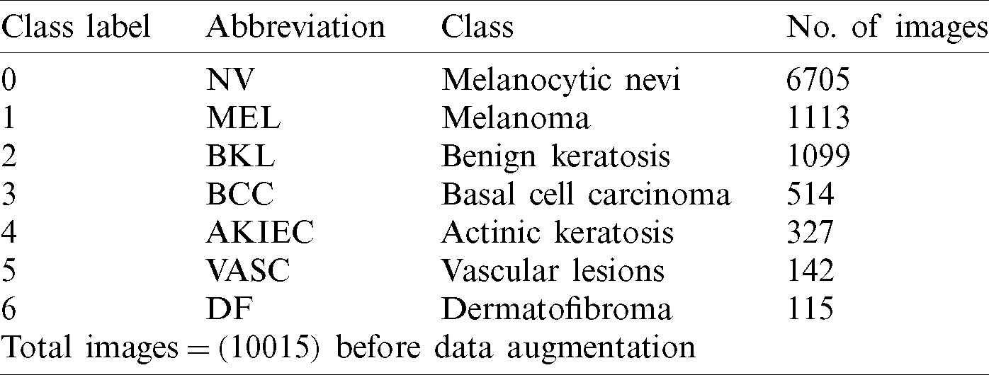
HAM10000 (Human Against Machine) (HAM) is a publicly available dataset [25]. HAM dataset is comprised of 10015 dermatoscopic images through the ISIC archive. The HAM dermatoscopic images are collected from different populations in different modalities. This dataset provides a diagnosis for seven pigmented lesion categories: Actinic keratosis (AKIEC), benign keratosis lesion (BKL), vascular lesions (VASC), basal cell carcinoma (BCC), dermatofibroma (DF), melanocytic nevi (NV), and melanoma (MEL). Most of these lesions are confirmed through histopathology. The lesion_id in the metadata file tracks the lesions within the dataset. The lesion images are diversely delivered. They were acquired different dermatoscopy types from various anatomic sites, i.e., nails and mucosa, from a sample of skin cancer patients, from several different institutions. Images were acquired under the Ethics Review Committee of the Medical University of Vienna and the University of Queensland. The HAM10000 dataset is also utilized as the training set for the ISIC 2018 challenge [25]. The distribution of seven pigmented lesions of HAM dermoscopic images is shown in Tab. 1.
Table 1: An overview of the HAM dataset and distribution of classes
Preprocessing steps are applied to cleanse and organize data before being fed into the model. Dataset images vary between high and low pixel range. Higher image values can result in different loss values from the lower range. Sharing the same model, weights, and learning rate require normalizing the dataset. Images pixels are scaled before the training phase in the deep learning architecture. Within experiments, images are rescaled to (224, 224, 3) using scaling techniques via the ImageDataGenerator class. Image pixel values are normalized to unify image samples. The pixel values in the range [0, 255] are normalized to the range [0, 1]. Without scaling, the high pixel range images will have many votes to update weights [22].
3.2.2 Training the Deep Network
Deep CNNs can learn hierarchically from low to high-level features automatically. Stacking the number of layers (depth) can enrich the levels of features. A deeper network can solve complex tasks and improve classification/recognition accuracy [26]. But, training the deeper network could face some difficulties, such as saturation/degrading of accuracy and vanishing/exploding gradients [27]. Utilizing deep residual pretrained architecture can solve both of these problems. Pre-trained model architecture facilitates training the deeper networks than the deeper framework used in [26]. ResNet50 is previously trained on ImageNet, composed of a large number of around 1.5 million natural scene images [27]. ResNet can reformulate network layers in terms of residual learning functions with a mapping reference to the input layer. Within ResNet, the stacked layers directly fit the desired mapping (residual mapping) [28].
The key idea of ResNet50 is to use identity mapping to predict the required to reach the final prediction of the previous layer outputs [27]. ResNet50 decreases the vanishing gradient effect using an alternate shortcut path to bypass. The identity mapping allows the model to flow through the unnecessary layers. This helps the model to overcome the overfitting problem to the training set [29].
Let the desired mapping be represented as
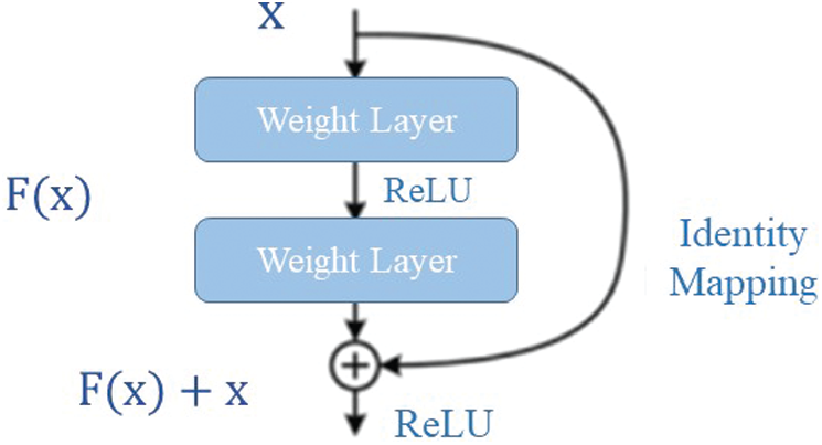
Figure 1: The residual identity mapping
The pre-trained deep learning model ResNet50 was used in training along with their weights. Because of the extensive training, it can facilitate training the deeper networks and gives better accuracies. The ResNet50 network consists of 50 layers deep with a small receptive field of
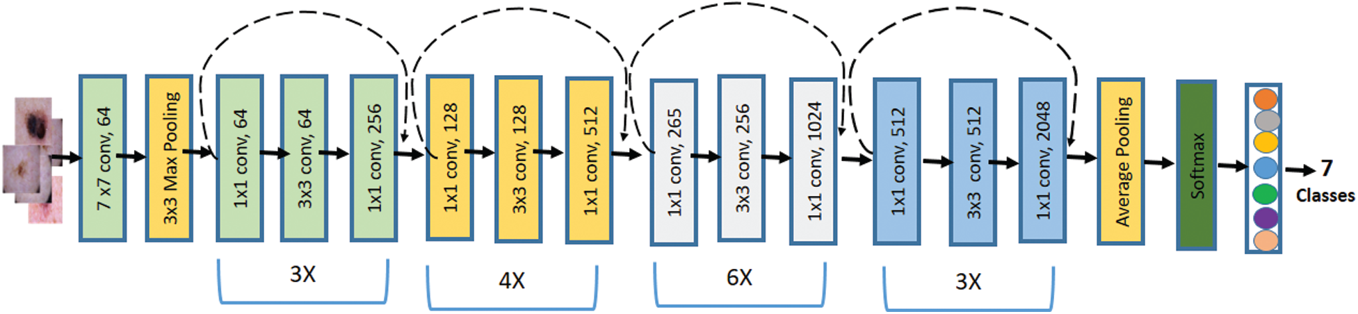
Figure 2: Block diagram of the Resnet50 network
Optimization has gained great importance, especially in deep learning, with the exponential growth of data. The large number of parameters within the deep layer network became a challenge to handle the complexities in adjusting the network’s parameters [30]. These optimization algorithms aim to fine-tune the results by utilizing various optimization techniques [31]. Setting the hyper-parameter affects the performance of the deep model. The development of optimization brings many efficient ways to adjust the hyper-parameters automatically [32]. Optimization methods by Adam optimizer have a significant influence on the learning performance rate [33]. Fine-tuning the deep architecture can have a considerable effect on the performance of a model [34]. Fine-tuning the deep architecture means the choice of deep training network, the layers involved within architecture and hyper-parameters for each layer, as well as the optimizers involved to enhance performance [27]. The proposed deep model utilizes various fine-tuning techniques, i.e., regularization, hyper-parameter tuning and batch normalization, transfer learning, cross-entropy optimization, and Adam optimizer.
Regularization Regularization techniques are applied to enhance the learnability of the network. Image data augmentation is used to synthesize new data to expand the used dataset. Creating new training data from existing training data can improve the performance and the model generalization ability [35]. Image augmentation increases the amount of available data by applying domain-specific techniques for creating transformed versions of images. These transformations can be flips, zooms, shifts, and much more. Augmentation can also transform invariant learning approaches and learn the model features that are also invariant to transforms, such as top-to-bottom to left-to-right and light levels in photographs [36].
Data preparation operations, i.e., image resizing and pixel scaling, are differentiated from image augmentation. Image augmentation is applied only to the training dataset, not to the validation or test dataset. But, data preparation must be consistently performed among all the model datasets [30]. A combination of affine image transformations was then performed, i.e., rotation, shifting, scaling (zoom in/out), and flipping to synthesize new data. The number of image samples was increased to a total of 12519 image datasets.
Hyperparameter Tuning and Batch Normalization Batch normalization achieves better optimization performance for convolutional networks [37]. Realizing the fixed distributions of inputs could remove the internal covariate shift’s effects, reduce the number of epochs required, and decrease generalization error [36]. Batch normalization can handle the internal covariate shift problem by standardizing the inputs to deep layers after each mini-batch. This can affect the learning process’s stability and eventually can reduce the number of training epochs required in training deep networks [38].
During training, batch normalization can be performed by computing the mean and standard deviation per mini-batch for each layer’s input variable to perform standardization. After training, the mean and standard deviation can be observed as mean values over the small mini-batches training dataset [38]. The mean and standard deviation of activation are calculated to normalize features by Eqs. (1) and (2), respectively [37].
where m represents the size of a mini-batch and xif is the fth feature of the ith sample. Using mini-batch mean and standard deviation, features can be normalized using Eq. (3) [37].
where
The backpropagation algorithm updates training based on the transformed inputs and adjusts the new scale and shifting parameters to reduce the model’s error [36]. Using batch normalization makes the network more stable with the adequate distribution of activation values throughout the training. Initialization of weights prior to training deep networks is a challenging problem. Achieving stability to training by batch normalization can handle the choice of weight initialization in training deep networks [38]. Batch normalization can be used as data preparation to standardize raw input data that have different scales [36]. Batch normalization has been widely used for training CNN to improve the distribution of the original inputs by scaling and shifting steps [37].
Transfer Learning The linear activation cannot learn complex mapping functions that can only be used in the output layer to predict a quantity, i.e., regression problems. Nonlinear activation functions, i.e., sigmoid and hyperbolic tangent, allow the nodes to learn more complex structures in the data [39]. A common problem with sigmoid and hyperbolic tangent functions is that they saturate. They saturate very high for a positive value, saturate to very low when for a negative value, and are sensitive to input value when z is near 0 [40].
For deep layers in large networks, using sigmoid and tanh function fail to receive suitable gradient information. The error is used to update the weights through the backpropagation, decreasing with additional layers [41]. It results in the vanishing gradient problem that prevents deep networks from learning effectively or knowing the suitable parameters to improve the cost function [39].
To train deep networks with deep layers, a specified activation function is needed. This activation function must act as a linear function to be sensitive to the activation input sum. It acts as a nonlinear function to allow the complex relationships within the data to be learned to avoid easy saturation [39]. To permit deep network development, major algorithms have significantly improved their performance by replacing hidden sigmoid units with piecewise linear hidden units, known as rectified linear units (ReLU) [41]. Because the ReLU is linear for half of the inputs and nonlinear for the others, it is recognized as a piecewise linear function [40].
a. ReLU
A ReLu activation is applied to all hidden layers. Three fully connected layers followed Max pooling layers. To achieve high training accuracy, the dropout layer and SoftMax classifier are connected at the last layers. After the dropout, the results are smoothed and fully connected via SoftMax. The feature mapping includes convolutions, ReLU activation function, and batch normalization. To retain a bounded feature map, the model is divided into separate blocks with stacked layers to reduce the feature map’s dimension. Hence, the model eventually prepared for 100 epochs for the dataset. ReLU activation function is the most common activation function used in networks with many layers. ReLU overcomes a lot of pf problems, i.e., vanishing gradient problem [41]. ReLU is presented by Eq. (5). The weights are updated by using the update rule in Eq. (6).
where w* is new weight computed based on current value w,
b. SoftMax
SoftMax enables the model to map certain classes to certain logits by maximizing the target classes’ logit values. It can also generate a discrete probability distribution for class outcomes [36]. This can lead to an effective training process and generating a useful machine-learning model. Besides normalization properties, SoftMax can be very useful for optimizing the network model [42]. SoftMax is a squashing function that results in vectors in the range (0, 1) and all sum up to one. These vectors are regarded as scores that represent class probability in multiclass classification [36]. Let the output scores denoted as s. The SoftMax function depends on all elements of the class, not for each class Si. The SoftMax function for an individual class Si can be given by Eq. (7) [4].
where Sj are scores inferred by the net for all classes. SoftMax ensures that the last layer of the network probabilities’ outputs have nonnegative real-valued probabilities with overall summation equals to one when no activation function is applied [36]. During iterative processes, the predictions are compared with the targets and summarized in a loss value. The improvement for the backpropagation is computed according to the loss value [4]. Performance improvement is subsequently performed using the optimizer and its idiosyncrasies. The iterative processes stop when the model achieves significant improvement in performance [36].
Optimization During iterative processes, the predictions are compared with the targets and summarized in a loss value. The improvement for the backpropagation is computed according to the loss value [36]. Performance improvement is subsequently performed using the optimizer and its idiosyncrasies. The iterative processes stop when the model achieves significant improvement in performance [4]. For this purpose, optimization techniques like Cross-Entropy Loss and Adam optimizer are used within the network architecture. For each trainable parameter, the optimizer subsequently adapts the parameter concerning the loss and intermediate layers [32]. The goal of optimization problems is to find the optimal mapping function f(x) that minimize the loss function L of the training samples of number N (Eq. (8)) [30].
where
where
where
where
a. Adaptive Moment Estimation (Adam)
Adam introduces an additional progressive to the SGD technique. Adam is an adaptive learning rate for each parameter, which integrates the adaptive learning method with the momentum methods [32]. Instead of storing the average of exponential decay of past squared gradients Vt, Adam keeps the average of exponential decay of past gradients mt (Eq. (14)), similar to the momentum method [33].
where
b. Cross-Entropy Loss
The choice of the loss function is also regarded as a significant part of the optimization. The model’s loss function can be used to estimate the current model state repeatedly. The loss function’s choice can affect weights in a suitable direction to reduce the next evaluation’s loss. The cross-entropy loss function is typically used for multiclass classification problems, where the target values are assigned integer values. The assigned target integer values are regarded as categorical within experiments [43]. Cross-entropy calculates a summarization score of the average difference between the actual and predicted values for all classes. The cross-entropy score is minimized towards the optimal value 0. Categorical cross-entropy L is defined by Eq. (17) [44].
where yc is the output based input x and weight wc, c is the index running over the classes number and tc is the number of occurrences of c. The cross-entropy loss function is evaluated mathematically under the inference framework of maximum likelihood. Maximizing the training set’s likelihood minimizes the cross-entropy loss as Eq. (18) [44].
where yc is the corresponding target value,
Experiments are performed using google Colaboratory (Colab) for accelerating deep learning GPU-centric applications. The hardware configuration for Colab accelerated runtime used to execute the coded program is GPU Nvidia K80, 12 GB RAM, 2496 CUDA cores.
The dermoscopic images of the HAM10000 dataset were first resized to
The evaluation results of the trained model are calculated using different performance metrics that are defined by Eqs. (19)–(24).
where TP denotes the number of positive instances that are labeled correctly. FP denotes the number of positive instances that are mislabeled. TN denotes the number of negative instances that are labeled correctly. FN denotes the number of negative instances that are mislabeled [45]. Precision and recall provide a true positive rate and positive predictive value, respectively. DSC provides the harmonic mean between precision and recall in a graphical representation between sensitivity and specificity measures. ROC curves, along with the associated AUC values, are also used in evaluation [9].
The first run was done by splitting the HAM dataset, which contains 12519 dermoscopic images of seven respective classes, into 80% for training and 20% for testing. The first run of training is done using 9514 dermoscopic images and 3005 for testing the HAM dataset concerning the seven classes: AKIEC, BKL, BCC, VASC, DF, MEL, and NV. The number of epochs for which the model was trained was 100. To evaluate the performance of the proposed framework, four performance metrics are computed for each class separately. Therefore, the average for these values is computed. The confusion matrix of this experiment is shown in Fig. 3.
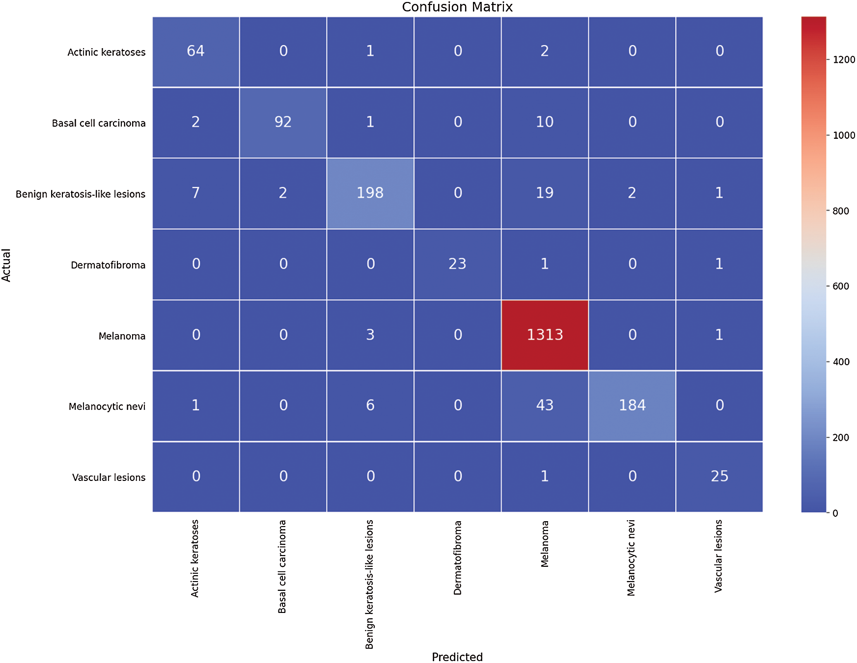
Figure 3: The confusion matrix for the first run
The four outcomes of the confusion matrix for the first run experiment are used to evaluate the performance metrics results. The fined-tuned model’s performance in terms of the three performance metrics, i.e., precision, recall, and DSC, are outlined in Tab. 2.
Table 2: The first run performance evaluation
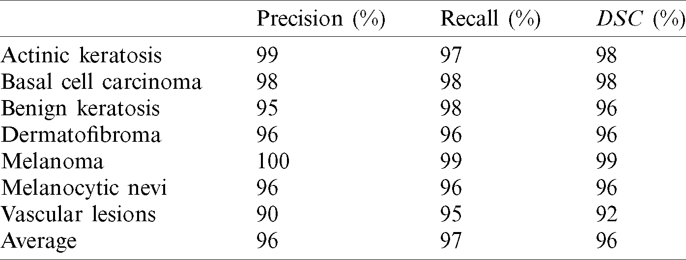
The performance metrics average is 98%, 96%, 97%, and 96.5% for accuracy, precision, recall, and DSC, respectively. Hence, the average for sensitivity and specificity is 98% and 100%, respectively. The second run is performed using the same conditions and architecture with another splitting ratio of 70% for training and 30% for testing using the hold-out method. The average values of performance metrics are computed. These values are 96.00% for the average accuracy of the seven classes, 90% for average accuracy of precision, 95.25% for recall, and 92.85% for average DSC. The confusion matrix of this experiment is shown in Fig. 4.
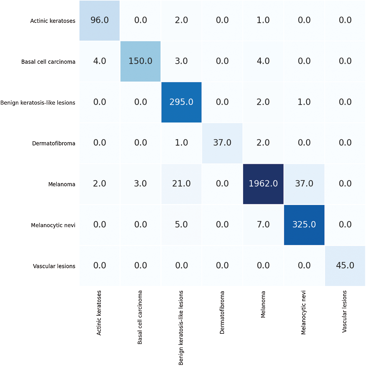
Figure 4: The confusion matrix for the second run
The confusion matrix outcomes for the second run experiment are used to evaluate the results in terms of performance metrics. The performance of the fined-tuned model in terms of the three performance metrics, i.e., precision, recall, and DSC are outlined in Tab. 3.
Table 3: The second run performance evaluation
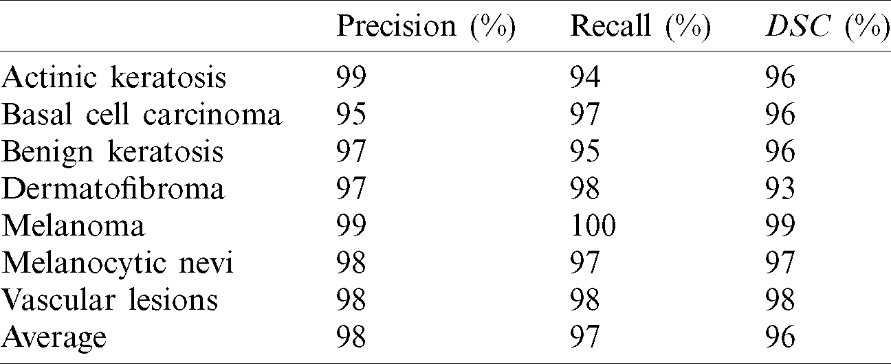
The performance metrics averages are 98%, 98%, 97%, and 96% for accuracy, precision, recall, and DSC, respectively. Hence, the averages for sensitivity and specificity are 98% and 100%, respectively. ROC curve is constructed to visualize the performance for the fine-tuned deep network in the classification of seven classes of skin cancer images. ROC curve for the fine-tuned deep and the seven respective classes is created by plotting the true positive rate (TPR) against false positive rate (FPR). Fig. 5a shows the relationship between sensitivity and specificity for the multiclass model. Moreover, for balanced results, macro and micro averaged ROC AUC scores are also calculated.
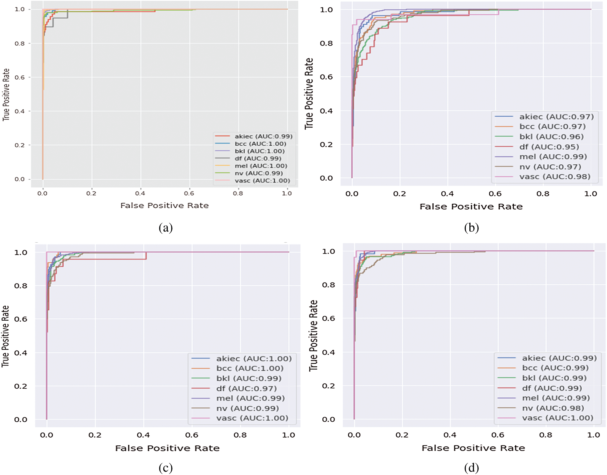
Figure 5: The area under the ROC curve for multiclass skin cancer (a) The proposed system, (b) InceptionV3, (c) VGG16, and (d) DenseNet
Other deep models of pre-trained networks on ImageNet are utilized for comparison, i.e., Inception v3 and VGG-16. Inception v3 and VGG-16 networks were re-trained using HAM dataset along with its seven respective classes. The Inception v3 layers’ architecture replaces top layers with one average-pooling layer that averages out the channel values across the 2D feature map. The inception module includes two fully connected and the SoftMax layer at the last layer to categorize the results within the seven respective classes. The inception module contains filters of
The VGG-16 network consists of 16 convolution layers with a small receptive field of
Table 4: The deep network models performance comparison
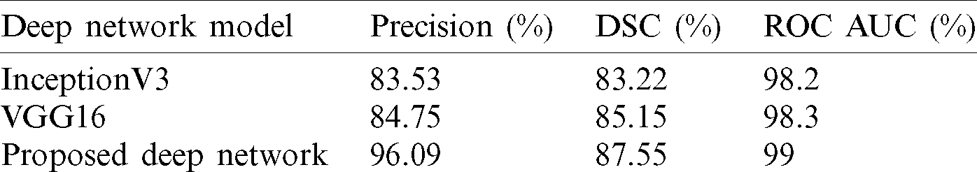
Tabs. 3 and 4 show the proposed deep network model’s performance among two different runs for testing the proposed model using two hold-out methods. The proposed model’s performance is presented for seven respective classes, which shows promising results in recognizing different skin cancer lesions. The two runs’ average results are listed in Tab. 5, which presents superior results against Inception v3 and VGG-16 deep models. The proposed deep model achieved a weighted average value of precision of 88.77%, DSC average of 87.55%, and ROC AUC average of 99%. In comparison, Inception v3 and VGG-16 deep models achieved 83.53% and 84.75% for precision, respectively. For DSC, they achieved 83.22% and 85.15%, respectively. For ROC AUC, they achieved 98.2% and 98.32, respectively.
Table 5: ROC AUC evaluation for deep comparative networks on each diagnostic class
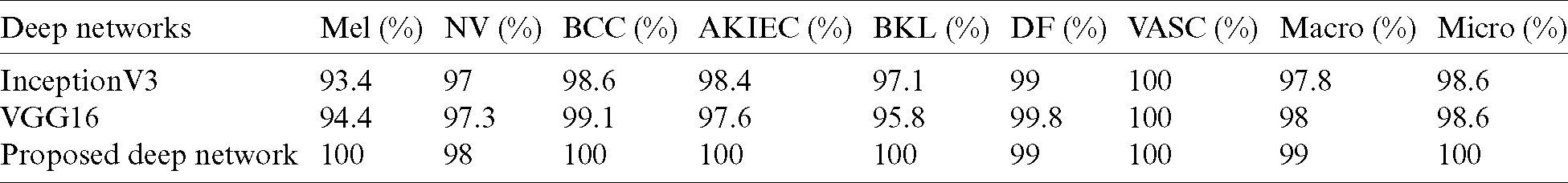
The ROC AUC values for each class shown in Tab. 5 are as follows: For melanoma and AKIEC classes, the proposed deep network scored the best with 99% and 100%, respectively. Also, for typical nevi and benign keratosis categories, they achieved higher AUC with 98% and 100% values, respectively. For basal cell carcinoma, VGG16 achieved higher AUC with the values of 99.1% than the proposed deep network and InceptionV3 values of 99% and 98.6%, respectively. For dermatofibroma cases, VGG16 achieved higher AUC with the values of 99.8% than the proposed deep network and InceptionV3 values of 99% and 99%, respectively. For vascular lesions categories, the proposed deep network, VGG16, and InceptionV3 entirely achieved 100%. ROC curve for the fine-tuned deep network in the classification of seven classes of skin cancer images in Fig. 5a shows superior performance compared to the ROC AUC for the comparative deep network models in other subfigures.
This study investigated the capability of deep learning in the multi-classification of 7 primary skin lesions. Performance evaluation using the pre-trained ResNet50 network on HAM dermoscopic images (12519 in total) outperforms other robust networks. A variety of fine-tuning techniques have been investigated for enhancing diagnosis performance, such as regularization, batch normalization, and hyperparameter optimization. Adam optimizer and cross-entropy loss function are also utilized with optimal parameters. The developed deep model has compared two powerful models, i.e., InceptionV3 and VGG16, for evaluation. The proposed fine-tuned deep learning model shows that fine-tuning networks can achieve better diagnostic accuracy than other powerful techniques. Although the utilized dataset is highly unbalanced, the model obtained promising results. These models can be easily implemented to assist dermatologists. A more diverse skin lesion categories dataset can be further investigated for future work. Also, the use of metadata for the images can be useful to enhance the diagnosis accuracy.
Funding Statement: The authors received no specific funding for this study.
Conflicts of Interest: The authors declare that they have no conflicts of interest to report regarding the present study.
1. T. J. Brinker, A. Hekler, A. Hauschild, C. Berking and J. S. Utikal. (2019). “Comparing artificial intelligence algorithms to 157 German dermatologists: The melanoma classification benchmark,” European Journal of Cancer, vol. 111, no. 10151, pp. 30–37. [Google Scholar]
2. M. N. Bajwa, K. Muta, M. I. Malik, S. A. Siddiqui and S. Ahmed. (2020). “Computer-aided diagnosis of skin diseases using deep neural networks,” Applied Sciences, vol. 10, no. 7, pp. 2488. [Google Scholar]
3. T. J. Brinker, A. Hekler, A. H. Enk, J. Klode and P. Schrüfer. (2019). “A convolutional neural network trained with dermoscopic images performed on par with 145 dermatologists in a clinical melanoma image classification task,” European Journal of Cancer, vol. 111, no. 10151, pp. 148–154. [Google Scholar]
4. A. A. Adegun and S. Viriri. (2020). “Deep learning-based system for automatic melanoma detection,” IEEE Access, vol. 8, pp. 7160–7172. [Google Scholar]
5. A. Hekler, J. S. Utikal, A. H. Enk, W. Solass and T. J. Brinker. (2019). “Deep learning outperformed 11 pathologists in the classification of histopathological melanoma images,” European Journal of Cancer, vol. 118, no. 10151, pp. 91–96. [Google Scholar]
6. L. Bi, J. Kim, E. Ahn, A. Kumar, D. Feng et al. (2019). , “Step-wise integration of deep class-specific learning for dermoscopic image segmentation,” Pattern Recognition, vol. 85, pp. 78–89. [Google Scholar]
7. P. Tschandl, C. Sinz and H. Kittler. (2019). “Domain-specific classification-pretrained fully convolutional network encoders for skin lesion segmentation,” Computers in Biology and Medicine, vol. 104, no. 3, pp. 111–116. [Google Scholar]
8. A. G. Pacheco, A.-R. Ali and T. Trappenberg. (2019). “Skin cancer detection based on deep learning and entropy to detect outlier samples,” ArXiv, vol. abs/1909.04525, pp. 1–6. [Google Scholar]
9. A. Mahbod, G. Schaefer, I. Ellinger, R. Ecker, A. Pitiot et al. (2019). , “Fusing fine-tuned deep features for skin lesion classification,” Computerized Medical Imaging and Graphics, vol. 71, no. 4, pp. 19–29. [Google Scholar]
10. A. Mahbod, G. Schaefer, C. Wang, R. Ecker and I. Ellinge. (2019). “Skin lesion classification using hybrid deep neural networks,” in 2019 IEEE Int. Conf. on Acoustics, Speech and Signal Processing, Brighton, United Kingdom. [Google Scholar]
11. T. Y. Tan, L. Zhang and C. P. Lim. (2020). “Adaptive melanoma diagnosis using evolving clustering, ensemble and deep neural networks,” Knowledge-Based Systems, vol. 187, no. 15, pp. 104807. [Google Scholar]
12. T. N. Sainath, B. Kingsbury, A. Mohamed, G. E. Dahl and B. Ramabhadran. (2013). “Improvements to deep convolutional neural networks for LVCSR,” CoRR, vol. abs/1309.1501, pp. 315–320. [Google Scholar]
13. K. He, X. Zhang, S. Ren and J. Sun. (2015). “Delving deep into rectifiers: Surpassing human-level performance on imagenet classification,” CoRR, vol. abs/1502.01852, pp. 1026–1034. [Google Scholar]
14. H. Zheng, Z. Yang, W. Liu, J. Liang and Y. Li. (2015). “Improving deep neural networks using softplus units,” in 2015 Int. Joint Conf. on Neural Networks, Killarney, Ireland, pp. 1–4. [Google Scholar]
15. Y. Chen, M. W. Hoffman, S. G. Colmenarejo, M. Denil, T. P. Lillicrap, M. Botvinick and N. Freitas. (2017). “Learning to learn without gradient descent by gradient descent,” Proc. of the 34th Int. Conf. on Machine Learning, PMLR, vol. 70, pp. 748–756. [Google Scholar]
16. Y. Bengio. (2012). “Practical recommendations for gradient-based training of deep architectures,” in Neural Networks: Tricks of the Trade, 2nd ed. Berlin, Heidelberg: Springer Berlin Heidelberg, pp. 437–478. [Google Scholar]
17. D. Jakubovitz, R. Giryes and M. R. Rodrigues. (2018). “Generalization error in deep learning,” CoRR, vol. abs/1808.01174, pp. 1–33. [Google Scholar]
18. Y. Bengio, P. Lamblin, D. Popovici and H. Larochelle. (2007). “Greedy layer-wise training of deep networks,” in Proc. of the 19th Int. Conf. on Neural Information Processing Systems, Cambridge, MA, Unites States: MIT Press. [Google Scholar]
19. B. N. Walker, J. M. Rehg, A. Kalra, R. M. Winters and A. Dascalu. (2019). “Dermoscopy diagnosis of cancerous lesions utilizing dual deep learning algorithms via visual and audio (sonification) outputs: Laboratory and prospective observational studies,” EBioMedicine, vol. 40, no. 10151, pp. 176–183. [Google Scholar]
20. G. Paolino, M. Donati, D. Didona, S. Mercuri and C. Cantisani. (2017). “Histology of non-melanoma skin cancers: An update,” Biomedicines, vol. 5, no. 4, pp. 71. [Google Scholar]
21. T. J. Brinker, A. Hekler, A. H. Enk, C. Berking and J. S. Utikal. (2019). “Deep neural networks are superior to dermatologists in melanoma image classification,” European Journal of Cancer, vol. 119, no. 10151, pp. 11–17. [Google Scholar]
22. T. J. Brinker, A. Hekler, A. H. Enk and C. von Kalle. (2019). “Enhanced classifier training to improve precision of a convolutional neural network to identify images of skin lesions,” PLoS ONE, vol. 14, no. 6, pp. e0218713. [Google Scholar]
23. M. A. Kassem, K. M. Hosny and M. M. Fouad. (2020). “Skin lesions classification into eight classes for ISIC, 2019 using deep convolutional neural network and transfer learning,” IEEE Access, vol. 8, pp. 114822–114832. [Google Scholar]
24. A. Naeem, M. S. Farooq, A. Khelifi and A. Abid. (2020). “Malignant melanoma classification using deep learning: Datasets, performance measurements, challenges and opportunities,” IEEE Access, vol. 8, pp. 110575–110597. [Google Scholar]
25. P. Tschandl. (2018). “The HAM10000 dataset, a large collection of multi-source dermatoscopic images of common pigmented skin lesions,” . https://github.com/ptschandl/HAM10000_dataset (Accessed 3 February 2021). [Google Scholar]
26. M. S. Hanif and M. Bilal. (2020). “Competitive residual neural network for image classification,” ICT Express, vol. 6, no. 1, pp. 28–37. [Google Scholar]
27. K. He, X. Zhang, S. Ren and J. Sun. (2016). “Deep residual learning for image recognition,” in 2016 IEEE Conf. on Computer Vision and Pattern Recognition, Las Vegas, NV, USA, pp. 1. [Google Scholar]
28. S. R. Xiangyu Zhang Kaiming He and J. Sun. (2015). “Deep residual learning for image recognition,” . https://arxiv.org/abs/1512.03385. [Google Scholar]
29. D. Theckedath and R. R. Sedamkar. (2020). “Detecting affect states using VGG16, ResNet50 and SE-ResNet50 networks,” SN Computer Science, vol. 1, no. 2, pp. 18. [Google Scholar]
30. S. T. Zouggar and A. Adla. (2020). “Optimization techniques for machine learning,” In: A. J. Kulkarni and S. C. Satapathy (Eds.) Optimization in Machine Learning and Applications. pp. 31–50. Singapore: Springer Singapore. [Google Scholar]
31. L. Bottou, F. E. Curtis and J. Nocedal. (2018). “Optimization methods for large-scale machine learning,” SIAM Review, vol. 60, no. 2, pp. 223–311. [Google Scholar]
32. E. M. Dogo, O. J. Afolabi, N. I. Nwulu, B. Twala and C. O. Aigbavboa. (2018). “A comparative analysis of gradient descent-based optimization algorithms on convolutional neural networks,” in 2018 Int. Conf. on Computational Techniques, Electronics and Mechanical Systems, Belgaum, India. [Google Scholar]
33. S. Sun, Z. Cao, H. Zhu and J. Zhao. (2020). “A survey of optimization methods from a machine learning perspective,” IEEE Transactions on Cybernetics, vol. 50, no. 8, pp. 3668–3681. [Google Scholar]
34. M. U. Yaseen, A. Anjum, O. Rana and N. Antonopoulos. (2019). “Deep learning hyper-parameter optimization for video analytics in clouds,” IEEE Transactions on Systems, Man and Cybernetics: Systems, vol. 49, no. 1, pp. 253–264. [Google Scholar]
35. A. Mahbod, G. Schaefer, C. Wang, R. Ecker and I. Ellinge. (2019). “Skin lesion classification using hybrid deep neural networks,” in ICASSP, 2019-2019 IEEE Int. Conf. on Acoustics, Speech and Signal Processing. [Google Scholar]
36. T. C. Pham, A. Doucet, C. M. Luong, C.-T. Tran and V. D. Hoang. (2020). “Improving skin-disease classification based on customized loss function combined with balanced mini-batch logic and real-time image augmentation,” IEEE Access, vol. 8, pp. 150725–150737. [Google Scholar]
37. Z. Yin, B. Wan, F. Yuan, X. Xia and J. Shi. (2017). “A deep normalization and convolutional neural network for image smoke detection,” IEEE Access, vol. 5, pp. 18429–18438. [Google Scholar]
38. Z. Fu, S. Li, X. Li, B. Dan and X. Wang. (2019). “Influence of batch normalization on convolutional neural networks in HRRP target recognition,” in 2019 Int. Applied Computational Electromagnetics Society Symp., China (ACES). [Google Scholar]
39. E. Goceri. (2019). “Analysis of deep networks with residual blocks and different activation functions: Classification of skin diseases,” in 2019 Ninth Int. Conf. on Image Processing Theory, Tools and Applications, Istanbul, Turkey. [Google Scholar]
40. F. Altaf, S. M. Islam, N. Akhtar and N. K. Janjua. (2019). “Going deep in medical image analysis: Concepts, methods, challenges and future directions,” IEEE Access, vol. 7, pp. 99540–99572. [Google Scholar]
41. K. C. Kirana, S. Wibawanto, N. Hidayah, G. P. Cahyono and K. Asfani. (2019). “Improved neural network using Integral-Relu based prevention activation for face detection,” in 2019 Int. Conf. on Electrical, Electronics and Information Engineering, Denpasar, Bali, Indonesia. [Google Scholar]
42. R. Yamashita, M. Nishio, R. K. Do and K. Togashi. (2018). “Convolutional neural networks: An overview and application in radiology,” Insights into Imaging, vol. 9, no. 4, pp. 611–629. [Google Scholar]
43. B. N. V., P. J. Shah, V. Shekar, H. R. Vanamala and A. V. K. (2020). “Detection of melanoma using deep learning techniques,” in 2020 Int. Conf. on Computation, Automation and Knowledge Management, Dubai, United Arab Emirates. [Google Scholar]
44. R. Koshy and A. Mahmood. (2019). “Optimizing deep CNN architectures for face liveness detection,” Entropy, vol. 21, no. 4, pp. 423. [Google Scholar]
45. M. R. Ibraheem and M. Elmogy. (2016). “Automated segmentation and classification of hepatocellular carcinoma using fuzzy C-Means and SVM,” Medical Imaging in Clinical Applications, vol. 651, pp. 193–210. [Google Scholar]
 | This work is licensed under a Creative Commons Attribution 4.0 International License, which permits unrestricted use, distribution, and reproduction in any medium, provided the original work is properly cited. |