DOI:10.32604/cmc.2021.016042
| Computers, Materials & Continua DOI:10.32604/cmc.2021.016042 | |
| Article |
Hybrid Deep Learning Architecture to Forecast Maximum Load Duration Using Time-of-Use Pricing Plans
1Department of KDN Electric power IT Research Institute, KEPCO KDN, Naju, 58217, Korea
2College of Technological Innovation, Zayed University, Abu Dhabi, UAE
3Department of Computer Science & Engineering, Chungnam National University, Daejeon, 34134, Korea
*Corresponding Author: Ki-Il Kim. Email: kikim@cnu.ac.kr
Received: 20 December 2020; Accepted: 28 January 2021
Abstract: Load forecasting has received crucial research attention to reduce peak load and contribute to the stability of power grid using machine learning or deep learning models. Especially, we need the adequate model to forecast the maximum load duration based on time-of-use, which is the electricity usage fare policy in order to achieve the goals such as peak load reduction in a power grid. However, the existing single machine learning or deep learning forecasting cannot easily avoid overfitting. Moreover, a majority of the ensemble or hybrid models do not achieve optimal results for forecasting the maximum load duration based on time-of-use. To overcome these limitations, we propose a hybrid deep learning architecture to forecast maximum load duration based on time-of-use. Experimental results indicate that this architecture could achieve the highest average of recall and accuracy (83.43%) compared to benchmark models. To verify the effectiveness of the architecture, another experimental result shows that energy storage system (ESS) scheme in accordance with the forecast results of the proposed model (LSTM-MATO) in the architecture could provide peak load cost savings of 17,535,700 KRW each year comparing with original peak load costs without the method. Therefore, the proposed architecture could be utilized for practical applications such as peak load reduction in the grid.
Keywords: Load forecasting; deep learning; hybrid architecture; maximum load duration; time-of-use
As cutting-edge technologies have been developed, there are significantly growing demands for electricity power. The increase in energy demands has been raising important issues, such as grid failure and peak load problem [1]. To overcome these issues, several techniques have been investigated. Demand response (DR) [2–4] is an incentive or price-based program provided by electric utility companies to reduce or shift energy demands from the peak period to the off-peak period. Virtual power plant (VPP) [5–7] is the method to combine several renewable resources, energy storage system (ESS) and power plants that can be activated as a single power plant for peak load shaving.
First of all, load forecasting [8] has been a crucial research field as its elementary technology of DR and VPP. In addition, the load forecasting has become an essential method for peak load shaving technologies and has contributed to grid stabilization, thereby enabling additional distributed energy resources to participate in the grid and improve the efficiency of electricity usage [9]. Especially, in order to achieve the ultimate goals such as peak load reduction in the grid, it necessary to employ the adequate model to forecast the maximum load duration (MLD) using time-of-use (TOU) pricing plans. The MLD is the peak load zone when electricity usage is fairly high at the maximum load zone of KEPCO TOU, the electricity usage fare policy of Korean utility company.
Recently, machine learning and deep learning models based on data-driven technologies have been regarded as an efficient load forecasting model. However, single machine learning or deep learning forecasting cannot easily avoid overfitting to the specific dataset and may fail to fit previously unseen data. Moreover, most commonly employed ensemble or hybrid models are not the most adequate models to forecast MLD based on KEPCO TOU.
Therefore, we propose a hybrid forecasting architecture incorporating three models: long short-term memory (LSTM) deep learning model, moving average, and K-fold-Correlation. The architecture can help to reduce overfitting using the highest performance model extracted from the hybrid combination process compared to single models. The main contributions of this study are summarized below.
• The proposed hybrid deep learning architecture can forecast the MLD based on TOU using binary combination technique for practical applications such as peak load reduction in a power grid.
• The experimental results of forecasting daily MLD indicate that the architecture could achieve the improved forecasting performance based on recall and accuracy compared to other benchmark models.
• The experimental results to verify the quantitative effectiveness for the proposed architecture show that the architecture employing energy storage system (ESS) operation scheme in accordance with the highest performance model provides peak load cost savings.
In Section 2, we present a general review of various methods of forecasting techniques. In Section 3, we describe the detailed technical results of the proposed architecture. Section 4 introduces benchmark models to identify the performance of proposed architecture. In Section 5, we address performance metrics. In Section 6, we discuss the experimental results of forecasting performance and peak load cost savings based on TOU. Finally, we discuss the effectiveness of the proposed architecture.
In the past 20 years, forecasting techniques have been utilized in various fields. The representative applied model types discussed in this section are summarized in Tab. 1.
Table 1: Summary of representative forecasting models applied to various fields
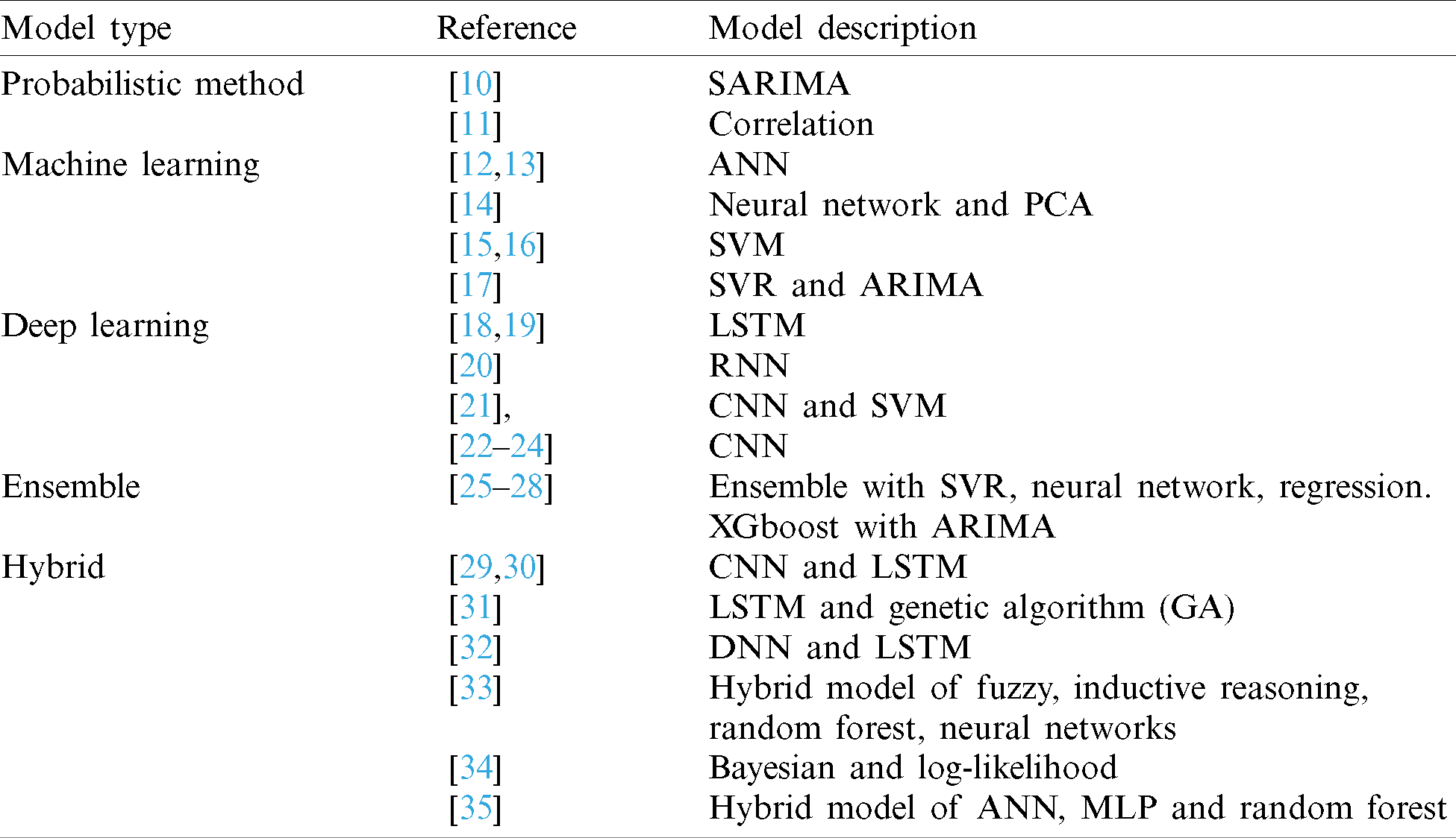
Typically, probabilistic models include moving average (MA), exponential smoothing (ES), autoregressive integrated moving average (ARIMA), and correlation. As an example of these models, there is a seasonal autoregressive integrated moving average (SARIMA) hybrid model with neural net- work suitable for processing nonlinear datasets with a variety of complex structures for forecasting short-term solar PV power generation [10]. Correlation analysis [11] is another stochastic method that analyzes statistical and mathematical correlations between two data sets for deriving meaningful insights. To measure the correlation between two probability variables, covariance is usually employed as follows:
The correlation coefficient is defined utilizing covariance as follows:
2.2 Machine Learning and Deep Learning Model
Basically, machine learning and deep learning models are the learning-based techniques that employ the supervised learning to forecast previously unseen data using features and labels that they learned from training data.
In case of applying optimized technique such as deterministic method, the optimized one is usually considered based on related multi variable parameters, constraints and mathematical model for forecasting, whereas machine learning and deep learning do not need the complicated mathematical model or several constraints when the amount of data and appropriate algorithm are utilized [8]. In addition, the learning process to find best parameters can be easily automated using useful machine learning and deep learning libraries.
There are several studies in renewable energy prediction regarding artificial neural network (ANN). In [12], a model based on ANN performs a-day-ahead forecast of the electricity profile usage for a commercial building. In [13], an ANN hybrid model is employed in wind speed forecasting for energy monitoring and effective management. Khan et al. [14] proposed a wind power forecasting method from significant features with a tensorflow-based neural network and principal component analysis (PCA) approach to decompose the raw historical wind speed data into reduced useful features.
Support vector machine (SVM) is a supervised learning method that performs classification and regression by distinguishing among two or more datasets with the concept of hyperplane. In [15], theoretical and experimental investigations are performed on the effects of integrity attacks that disrupt the training data with SVM and game theory. The article [16] reports a study utilizing machine learning with SVM related to carbon emissions prediction. The support vector regression (SVR) model employs the concepts of regression utilizing hyperplane and margin. In [17], SVR incorporates time series models, such as ARIMA, to predict energy demand.
Deep learning prediction techniques are recently employed to forecast periodic time-series electrical usage or patterns. Kong et al. [18] utilized LSTM to predict energy consumption to reflect the lifestyle of residents. Li et al. [20] proposed the RNN-based short-term method for forecasting PV power only by considering previous PV power data as input without weather information. In addition to prediction, in [19], LSTM is employed as a deep-learning-based method for generating syllable-level outputs. In [21], convolutional neural network (CNN) and SVM were employed as the base classifiers to forecast failure in energy sector utilizing textual data. Furthermore, in [22], CNN was employed to obtain wind power characteristics by convolution, kernel and pooling operations for 24 h-ahead wind power forecasting. Sun et al. [23] proposed a CNN-based solar prediction model for 15-min ahead PV output forecasting. Sanakoyeu et al. [24] proposed a technique for unsupervised learning of visual similarities between a large number of examples to analyze the shortcomings of exemplar learning on CNN.
Ensemble models are Bagging and Boosting with a combination of single machine learning models. Bagging and Boosting can obtain a higher performance than a single model through the learning process that combines a set of weak learners to produce a strong learner. Ensemble methods can be employed as a prediction model of energy usage of buildings [25]. In [26], it is proposed the ensemble model combining SVR, neural network, and linear regression learners for energy consumption forecast. Divina et al. [27] presented short-term forecasting results based on ensemble learning incorporating different learning mechanisms to achieve accurate prediction results. The XGboost model with ARIMA evaluated and forecasted the energy supply level and energy supply security index in [28].
A hybrid model is a method that combines various models with optimized techniques. In [29], a hybrid model combining CNN and LSTM model is employed on power de-mand value (key) forecasting with a context value (context). An integrated CNN with LSTM model was employed to fore- cast oncoming responses of wind turbine [30]. Bouktif et al. [31] developed a LSTM hybrid model employing the Genetic Algorithm (GA) to find optimal time lags and the number of layers to predict electricity consumption. In [32], electricity prices forecasting was proposed employing a hybrid deep neural network (DNN)-LSTM to simultaneously forecast day-ahead prices in several countries. In [33], a hybrid methodology was proposed to combine feature selection based on entropies and machine learning approaches such as fuzzy, inductive reasoning, random forest, and neural networks. In [34], a hybrid learning method for bayesian networks incorporating two-component mixture-based log-likelihood was performed for binary classification tasks. In [35], a financial time series volatility is forecasted through hybrid learning employing various models such as ANN, multilayer perceptron (MLP), and random forest (RF).
Basically, in [10–17], these studies addressed probabilistic- based or machine learning forecasting model not to consider forecasting MLD based on TOU that the proposed architecture wants to address. In [18–20], only single LSTM model was addressed for forecasting. In [21–24], these CNN models have commonly been applied as a feature extraction and a part of prediction module for forecasting. Ensemble [25–28] or hybrid models [29–35] among these studies do not consider achieving optimal results for forecasting the MLD based on KEPCO TOU for peak load reduction in the grid.
In this paper, to overcome these limitations, the proposed architecture can forecast MLD based on KEPCO TOU and the proposed architecture shows the improved forecasting performance compared to benchmark models and even a hybrid benchmark model.
3 Proposed Hybrid Architecture
In this section, the proposed hybrid architecture is introduced. We developed it as a hybrid framework as shown in Fig. 1. We utilized original electricity data (06.01.2015–08.02.2018) obtained from the Korea Electric Power Corporation Knowledge Data & Network (KEPCO KDN) headquarter located in Naju City, South Korea. The original dataset consists of electricity usages at each time zone (from 1 to 24 h) each date for all days. The data pattern analysis block for treating the entire dataset efficiently chooses which data type is more suitable as an input dataset between the electrical pattern of the same day for previous week and the electrical pattern for the previous day. In the data preprocessing block, the original data is preprocessed to predict MLD which the proposed architecture attempts to forecast. The entire dataset is divided into training data for building a prediction model and test data for testing. The ratio of training data and test data is 70% and 30% respectively.
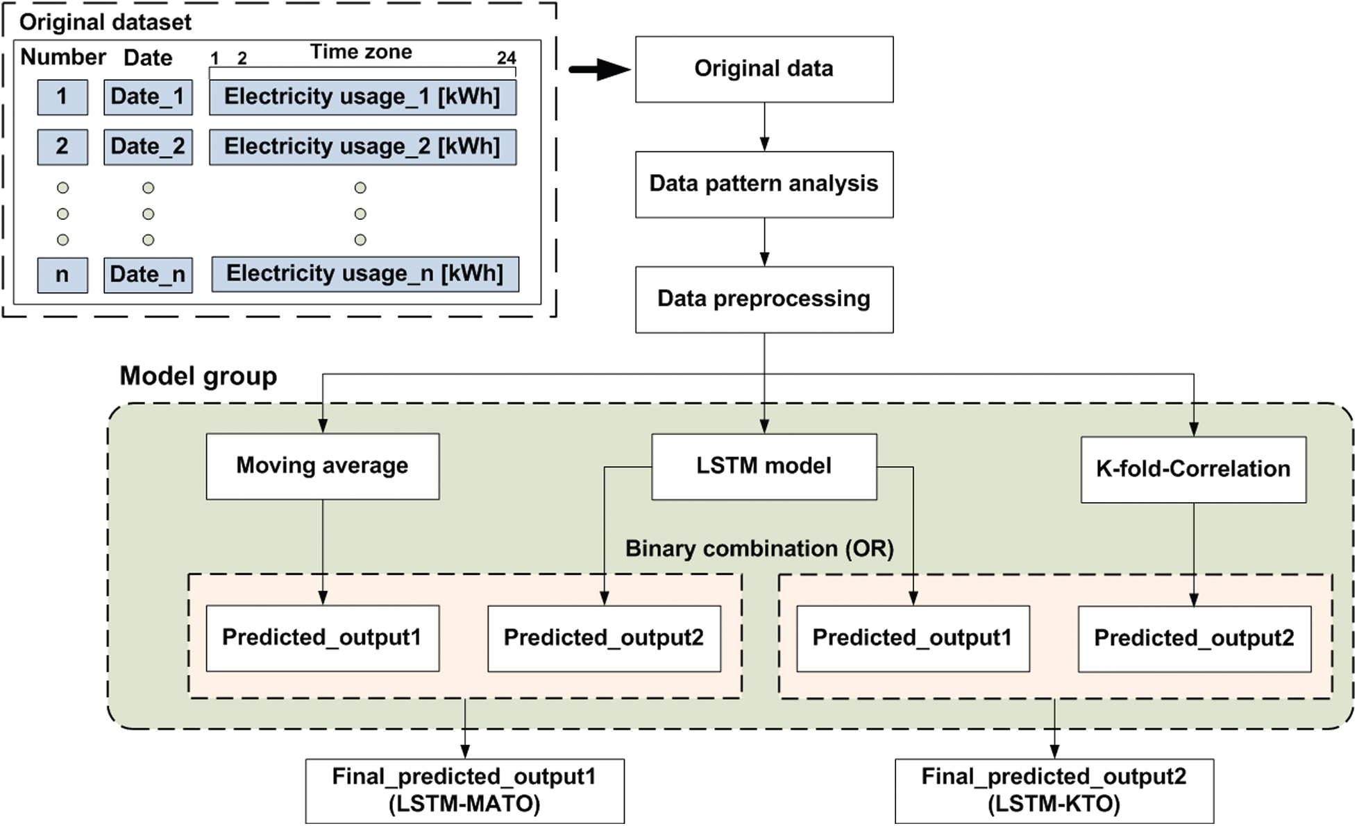
Figure 1: The proposed hybrid architecture incorporating three kinds of models
The model group block is composed of three models: MA, LSTM model, and K-fold-Correlation. The binary combination combines the results of the two models with an OR logical combination. Through the binary combination in the model group, the proposed architecture can provide two kinds of predicted outputs to fit newly measured electricity data continuously to reduce overfitting.
We generate two types of input datasets with the assumption the real electricity pattern is similar to the predicted pattern utilizing the same day for the previous week or the predicted one utilizing the previous day.
As shown in Fig. 2, it requires twice as long to train and test each model of the architecture if we utilize two types of datasets. To reduce training and testing time of each model, and to understand dataset characteristics efficiently, we analyze electricity usage patterns applied as a training dataset extracted from the original data employing the data pattern analysis block. Therefore, we can identify a more suitable data pattern as an input dataset in advance. From the analysis block result, we decide a type of dataset as an input for each model between two types of datasets, train and test models using extracted a dataset type. By applying this approach, we can reduce the time by up to 50%.
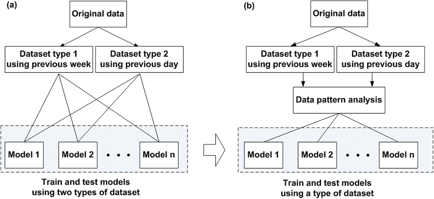
Figure 2: Two types of dataset: (a) without data pattern analysis, (b) using data pattern analysis
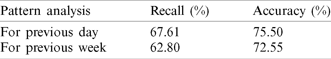
Tab. 2 explains the comparison results between actual electricity pattern in two cases: The predicted one using the same day for the previous week and the other using the previous day. As described in Tab. 2, we can see the higher performance in case of employing the electrical pattern for the previous day. Therefore, we apply the previous five days to input data format of the architecture instead of using data format for the same days (total of five days) during the previous five weeks from the analyzed results.
Table 2: The comparison results between actual pattern and two cases
In this section, we define the MLD based on TOU. As introduced in prior research, we utilize key parameters [36]: slope index (SI), cumulative slope (CS), and cumulative slope index (CSI).
The SI is defined as the variation of electricity usage divided by time zone. The SI is calculated as follows:
where n is the time interval; Pn is the electricity usage; Tnis the time zone [1.24] each day.
The CS is defined as the sum of the current SI and the previous CS. The CS is calculated as follows:
The CSI is defined as the ratio of CS divided by the maximum CS. The CSI is calculated as follows:
where CSmax is the highest CSn within the time zone [1.24] each day.
In this paper, we define the CSI value (= 1) when CSI
• The CSI value in the maximum load zone of KEPCO TOU
• One (= 1) when
Therefore, the MLD is the peak load zone when electricity usage is fairly high (
Table 3: The input dataset list for three models in the architecture and benchmark models
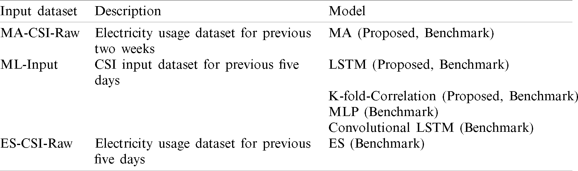
There are three models (MA, LSTM, and K-fold-Correlation) in the model group. As time-series data may exhibit uncertainty that is unpredictable, the model group makes two kinds of final predicted outputs (LSTM-MATO, LSTM-KTO) to overcome the limitation in this paper. LSTM-MATO employs MA and LSTM. The MA is used to smooth out the data fluctuation problem and get long term trends. The LSTM is used to make predictions based on time series data using deep learning method. LSTM-KTO employs LSTM and K-fold-Correlation. Especially, K-fold-Correlation is used to combine advantages of Perceptron and Correlation. Perceptron is a simple and efficient neural network model and Correlation method is a statistical interrelations analysis.
The MA is the simple probabilistic method to calculate average electrical usage at each time for all days during a specific period. The first step of the model operation is to calculate average electrical usage at each time for previous two weeks. Then, the CSI parameter can be extracted from the calculated average electricity usage. In the third step, we can find MLD (=1) when CSI value exceeds 80% at the maximum load zone of KEPCO TOU using extracted MA-CSI-Raw input dataset shown in Tab. 3. The MA is defined as follows:
where n is the number of samples for the last two weeks; Dt is the electricity usages.
The LSTM is the time series forecasting model of deep learning neural network. Fig. 3 explains the input data structure of LSTM model. The entire dataset consists of two sets: a training set that accounts for 70% and a test set that accounts for 30%. The “ymd” set denotes year, month and day attributes. The x_train set explains CSI input features and the number of x_train features is 30. Furthermore, xt_train set is the temperature features and the number of features is 30. The y_train set and y_test set consist of CSI labels and the size of each set is six. The input test set (x_test, xt_test) has the same structure as the training set structure with the difference of size (
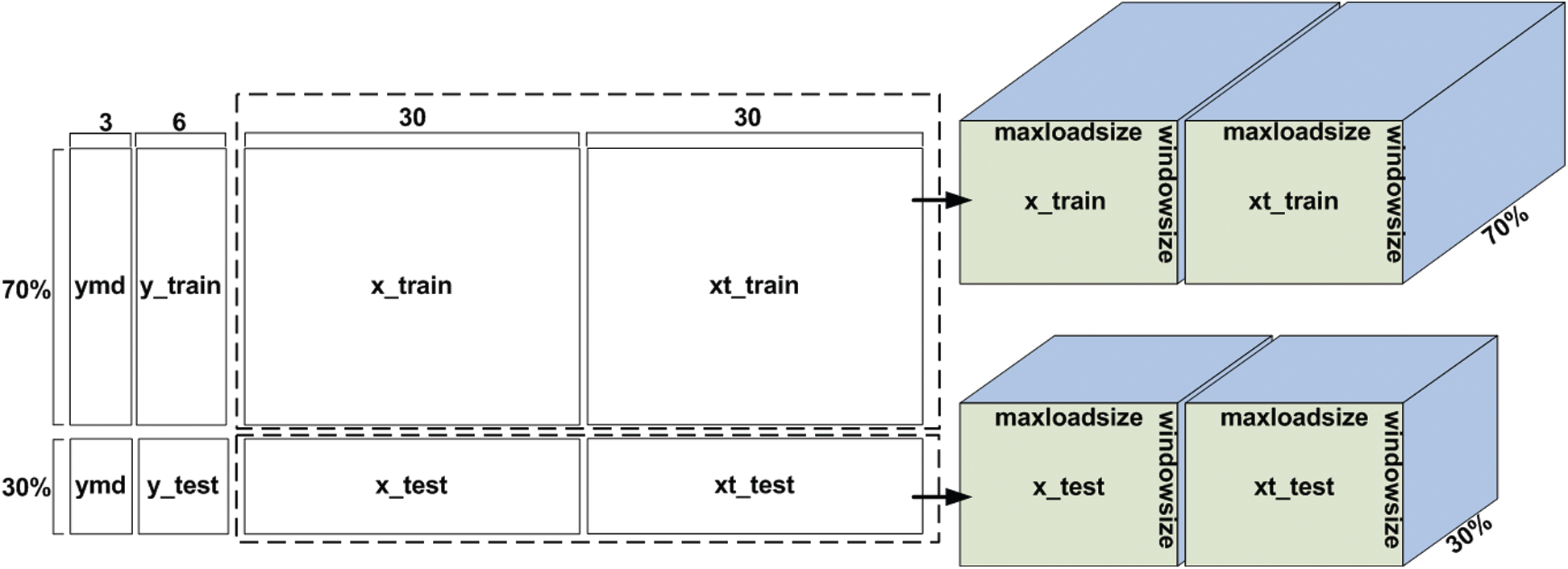
Figure 3: The input data structure of LSTM model
As an input of LSTM with three dimensions (3D) on the right side of two dimensions (2D) data structure, the total dimension of the training set is (
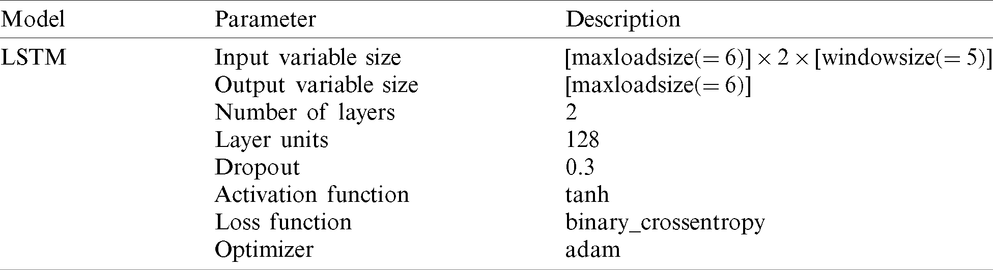
Tab. 4 shows the main parameters for designing LSTM model. The input variable size is 60 and output variable size is six. The hyperparameters optimized for the model are two layers, 128 layers units, 0.3 dropout, tanh activation function, binary_crossentropy loss function and adam optimizer.
Table 4: Main parameters for designing LSTM model
K-fold-Correlation is a proposed hybrid model to combine neural network and correlation analysis. To develop a simple and efficient model, we incorporate the neural network model of Perceptron and Correlation method that can perform statistical interrelations analysis. Algorithm 1 explains the operation principal of K-fold-Correlation model as follows:
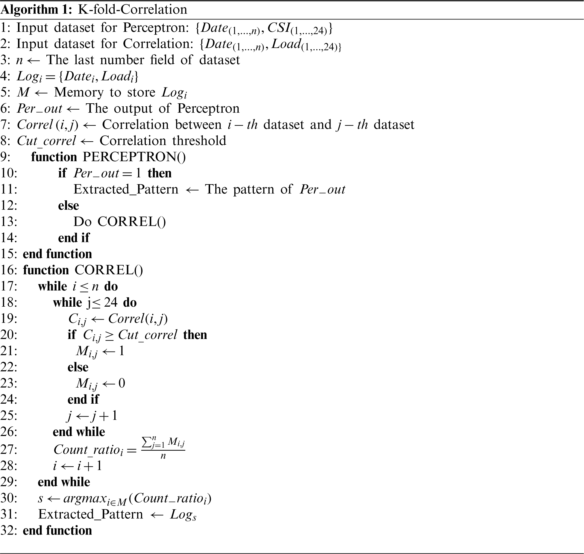
The first process of K-fold-Correlation is to perform the k-fold validation test (Leave-One-Out,
The binary combination combines the predicted outputs of the two single models by using a binary combination (OR). The first combination model (LSTM-MATO) employs MA and LSTM. The second combination model (LSTM-KTO) employs LSTM and K-fold-Correlation. The combination can be utilized to improve the forecasting ability of MLD as well as reduce overfitting through binary combination technique without biasing a single model.
We developed benchmark models to identify the performance of the proposed architecture. There are six benchmark models: MA, K-fold-Correlation, LSTM, ES, MLP, and Convolutional LSTM.
At first, three models (MA, K-fold-Correlation, and LSTM) are the benchmark models incorporating the proposed architecture to identify the synergistic effect of the hybrid model.
The ES is the prediction model to calculate electricity usage with different weights each date for previous five days. The ES is defined as follows:
where
Eq. (7) shows that the most recent data earns the largest weight and the old data receive the weight that decreases exponentially over time. CSI can be calculated using predicted electricity usage extracted from the ES model. If CSI value is over 80% in maximum load zone of KEPCO TOU, the time zone is set as MLD and if it is less than that, the zone is set as not MLD.
The MLP is an artificial neural network that generates outputs from a series of inputs. It features hidden layers connected by graphs plotted between the input and output layers. To optimize the model, the MLP employs backpropagation training the model. As shown in Tab. 5, the hyperparameters optimized for MLP are 0.001 learning rate, 3 hidden layers, gradient descent optimizer, sigmoid activation function and 2000 epochs. Regarding the input variable, maxloadsize (= 6) denotes there are six maximum load zones of KEPCO TOU each day and windowsize (= 5) denotes the input dataset for the previous five days.
Table 5: Main parameters for designing benchmark models (MLP, Convolutional LSTM)
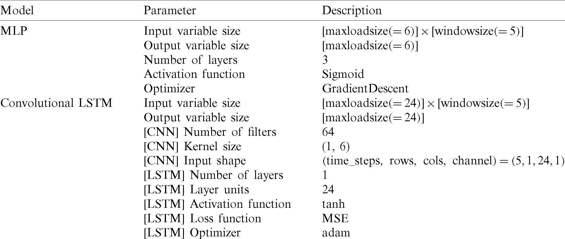
Convolutional LSTM is the deep learning model incorporating CNN and LSTM. The output from CNN that can extract input features is employed as an input of LSTM. Tab. 5 shows the model description for convolutional LSTM using keras deep learning library. The input variable size is 120 incorporating maxloadsize (= 24) and windowsize (5). Specifically, the maxloadsize is 24 which denotes 24 hour each day as an input dataset. Output variable size is maxloadsize (= 24). The hyperparameters optimized for the model are 64 filters, (1,6) kernel size, (5, 1, 24, 1) input shapes for CNN. The hyperparameters for LSTM are one layer, 24 layers unit, tanh activation function, mean squared error (MSE) loss function and adam optimizer.
Basically, we need the adequate model to forecast the MLD based on TOU for peak load reduction in the grid. The proposed architecture is to predict MLD, the peak load zone when electricity usage is fairly high (CSI
Table 6: KEPCO TOU: (1) Electricity usage fare for load zone and season
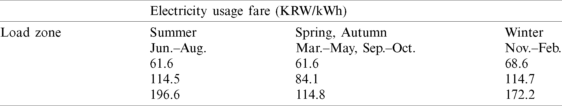
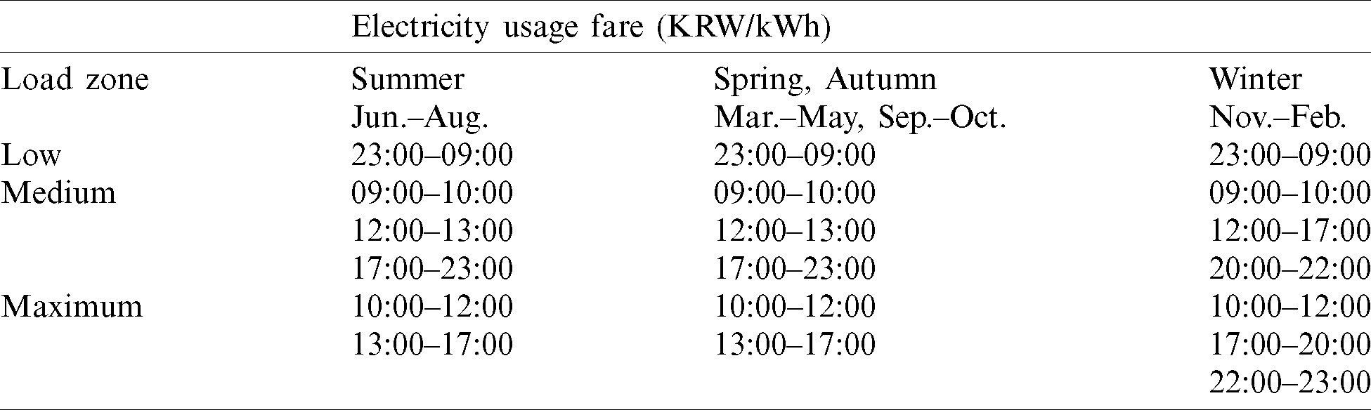
Table 7: KEPCO TOU: (2) Time zone for load and season
For this reason, the performance metrics are configured to predict MLD as accurately as possible, employing the proposed preprocessed CSI datasets featured in binary classified attributes (MLD or not MLD).
A confusion matrix is generally utilized to analyze the performance of a binary classification model as machine learning and deep learning. When CSI value is over 80% at the maximum load zone of KEPCO TOU, we define the load zone as MLD (= 1), and if the value less than 80% or the value is not at the maximum load zone of KEPCO TOU, we set it as not MLD (= 0). Therefore, the binary classification matrix can be the best performance metrics to classify MLD attributes. Each class of performance metrics can be represented as follows:
• True Positive (TP): The load zone is also MLD when the model predicts MLD.
• True Negative (TN): The load zone is not MLD when the model predicts not MLD.
• False Positive (FP): The load zone is not MLD when the model predicts MLD.
• False Negative (FN): The load zone is MLD when the model predicts not MLD.
Using four cases, three performance evaluation indexes can be introduced as follows:
In this article, we set the performance metrics to achieve a high hit rate of the MLD detected rather than the hit rate of MLD precise detections. Considering these metrics, the recall turns out to be an important performance index and the accuracy index is also an important factor in any case. Therefore, we choose the model with the highest average of recall and accuracy among the models.
In this section, we examine the experimental results of the proposed architecture. In the first experiment, we compare the proposed architecture models with other benchmark models to find the highest performance model. In the second experiment, we analyze peak load costs savings of the highest performance model quantitatively. Finally, we discuss forecasting effectiveness of the proposed architecture.
6.1 Forecasting Performance of the Proposed Architecture
Tab. 8 explains the experimental results of the proposed models in the architecture and benchmark models.
Table 8: The experimental results of proposed models in the architecture and benchmark models
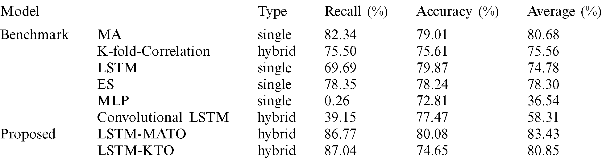
The experimental results of LSTM-MATO show the synergistic effect of the hybrid model. The LSTM-MATO could achieve the highest recall (86.77%), the highest accuracy (80.08%) compared with other benchmark models and show the highest average of recall and accuracy (83.43%) among models. The LSTM-KTO obtained the highest recall (87.04%) among models, whereas the model could not show the improved accuracy (74.65%).
Especially, the proposed model (LSTM-MATO) obtained scores over 80% for recall, accuracy, and an average of recall and accuracy. Therefore, LSTM-MATO is the highest performance model with the highest average of recall and accuracy among the models for peak load cost savings.
6.2 Peak Load Cost Savings based on TOU
Battery storage dispatch strategy incorporating TOU and demand charge management was developed and was utilized as an application of peak load shaving [37]. The strategies of this article indicate that ESS charges at off-peak and discharges at on-peak. Uddin et al. [1] explained peak load shaving techniques through the process of charging ESS when demand is low and discharging when demand is high. Considering the above strategies of ESS operation, it is important to set ESS discharging operation at the peak and charging operation at night when demand is low. In this article, to operate ESS for peak load costs reduction, ESS operating scheme is configured following the predicted MLD from the architecture. It indicates ESS discharges in operation at the peak when electricity usage is high (CSI
• ESS charges at night in the low load zone of KEPCO TOU.
• ESS discharges at MLD (= 1) that the model in the architecture predicts.
Using the ESS operating scheme, we calculate the cost savings of LSTM-MATO to analyze peak load cost savings quantitatively.
Algorithm 2 explains the peak load cost savings calculation. In the beginning, we prepare the original CSI dataset and the predicted MLD dataset of LSTM-MATO. Then, comparing CSI at the maximum load zone of KEPCO TOU with predicted MLD, the count of cost-saving increases whenever the CSI (= 1) at the maximum load zone of KEPCO TOU and predicted MLD (= 1) are equal. Cost savings are finally calculated using the count of cost-saving, an average of electricity usage and the usage fare difference between the maximum and the low load zone of KEPCO TOU.
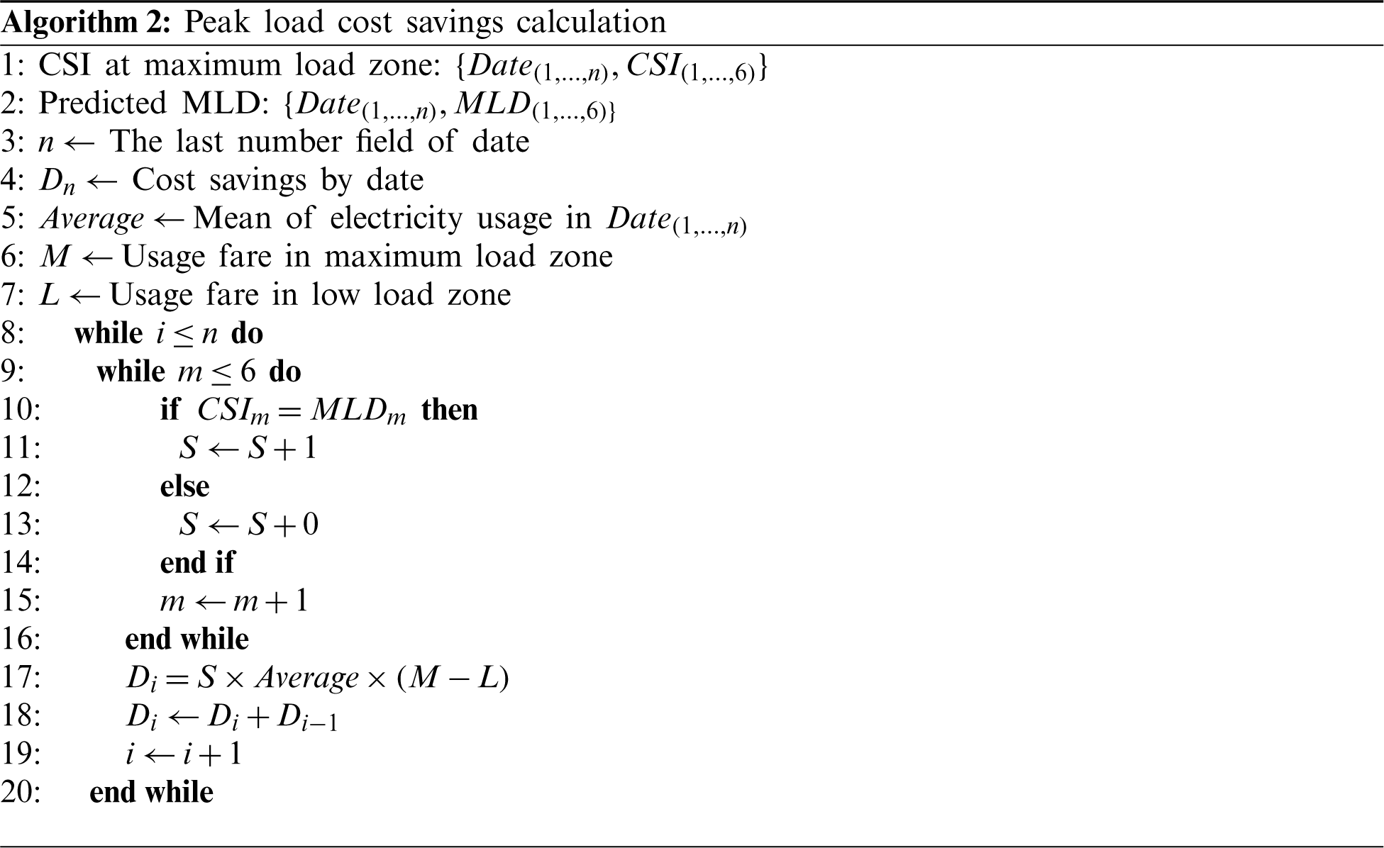
From the Algorithm 2, it is expected to reduce the peak load costs (= 17, 535, 700 KRW) each year comparing with original peak load costs without the method when we apply the predicted results of LSTM-MATO in the proposed architecture to ESS scheme and the ESS also operates in accordance with the scheme thoroughly.
Fig. 4 shows the comparison results between peak load costs without the method and peak load costs with the proposed method each day (from 08.23.2017 to 08.02.2018) marked as an index (from 1 to 236) using the Algorithm 2.
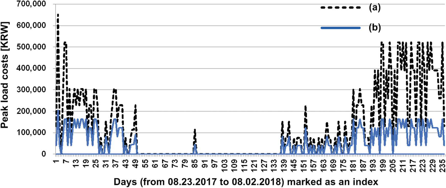
Figure 4: The results between (a) and (b): (a) without the method, (b) with the proposed method
The first benefit of the proposed forecasting technique is that the architecture can offer the high potential to improve the stability of the grid with peak load costs reduction. Peak load cost reduction means to shave the peak load at the peak load zone in each household or each office building.
Fig. 5 illustrates the power grid concept that several office buildings or households to employ ESS operation scheme and ESS. When we consider each office building or each household to achieve each own peak load costs reduction based on TOU using the proposed method efficiently, the proposed approach can offer the potential that the aggregate peak load costs reduction effects lower peak loads at the maximum load zone based on TOU of the whole office building or households in the grid.
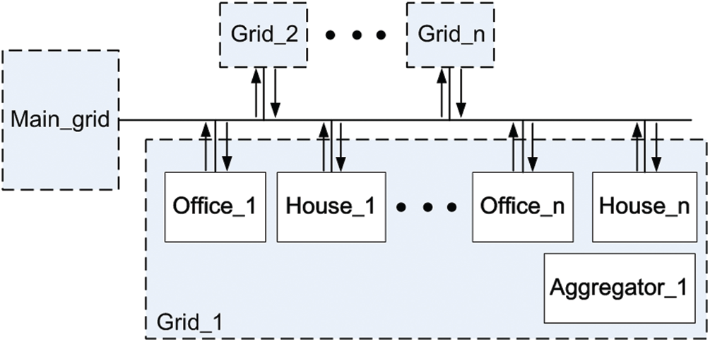
Figure 5: The power grid concept of office buildings and households to employ ESS operation scheme
The second benefit of the proposed architecture is that the electricity aggregators can provide more efficient DR signals to electricity consumers than before. Recently, the demand response program has been investigated in [2–4] based on the real power market.
In this scenario, when the proposed architecture is applied to DR program efficiently, electricity aggregators can provide more efficient DR signals to electricity consumers than before. For example, the aggregator would send the higher price signal when the aggregate forecasting results represent the peak load at the maximum load zone of TOU.
In this article, we proposed a hybrid architecture incorporating MA, LSTM model, and K-fold-Correlation. The proposed architecture combined the results of the two models with an OR logical combination to fit newly measured electricity data continuously to reduce overfitting. Especially, the proposed LSTM-MATO in the architecture showed the synergistic effect as a hybrid model. The LSTM-MATO showed the highest recall (86.77%), the highest accuracy (80.08%), and the highest average of recall and accuracy (83.43%) compared to MA and LSTM benchmark models incorporating LSTM-MATO. Comparing with other benchmark models (K-fold-Correlation, ES, MLP, and Convolutional LSTM), the proposed model (LSTM-MATO) obtained scores over 80% for recall, accuracy, and an average of recall and accuracy. On the contrary, other benchmark models obtained scores under 80%. To verify the quantitative effectiveness of the proposed architecture, another experimental result showed that the proposed architecture could provide peak load cost savings of 17,535,700 KRW each year using ESS operation scheme, in accordance with the forecasting results of the highest performance model (LSTM-MATO). The proposed hybrid architecture can be utilized to forecast the MLD based on TOU for practical applications such as peak load reduction in the grid. In the near-future research, it is expected that the proposed architecture will be available as a forecasting application for peak load reduction in the real power grid.
Funding Statement: This work was supported by Institute for Information & communications Technology Planning & Evaluation (IITP) grant funded by the Korea government (MSIT)(No.2019-0-01343, Training Key Talents in Industrial Convergence Security) and Research Cluster Project, R20143, by Zayed University Research Office.
Conflicts of Interest: The authors declare that they have no conflicts of interest to report regarding the present study.
1. M. Uddin, M. F. Romlie, M. F. Abdullah, S. A. Halim, A. H. A. Bakar et al. (2018). , “A review on peak load shaving strategies,” Renewable and Sustainable Energy Reviews, vol. 82, pp. 3323–3332. [Google Scholar]
2. B. Parrish, P. Heptonstall, R. Gross and B. K. Sovacool. (2020). “A systematic review of motivations, enablers and barriers for consumer engagement with residential demand response,” Energy Policy, vol. 138, no. 4, pp. 1–11. [Google Scholar]
3. A. R. Jordehi. (2019). “Optimisation of demand response in electric power systems, A review,” Renewable and Sustainable Energy Reviews, vol. 103, pp. 308–319. [Google Scholar]
4. N. Karthikeyan, J. R. Pillai, B. Bak-Jensen and J. W. Simpson-Porco. (2019). “Predictive control of flexible resources for demand response in active distribution networks,” IEEE Transactions on Power Systems, vol. 34, no. 4, pp. 2957–2969. [Google Scholar]
5. M. J. Kasaei, M. Gandomkar and J. Nikoukar. (2017). “Optimal management of renewable energy sources by virtual power plant,” Renewable Energy, vol. 114, no. 2, pp. 1180–1188. [Google Scholar]
6. S. Hadayeghparast, A. S. Farsangi and H. Shayanfar. (2019). “Day-ahead stochastic multi-objective economic/emission operational scheduling of a large scale virtual power plant,” Energy, vol. 172, pp. 630–646. [Google Scholar]
7. A. Rosato, M. Panella, R. Araneo and A. Andreotti. (2019). “A neural network based prediction system of distributed generation for the management of microgrids,” IEEE Transactions on Industry Applications, vol. 55, no. 6, pp. 7092–7102. [Google Scholar]
8. C. Deb, F. Zhang, J. Yang, S. E. Lee and K. W. Shah. (2017). “A review on time series forecasting techniques for building energy consumption,” Renewable and Sustainable Energy Reviews, vol. 74, pp. 902–924. [Google Scholar]
9. J. S. Chou and D. S. Tran. (2018). “Forecasting energy consumption time series using machine learning techniques based on usage patterns of residential householders,” Energy, vol. 165, no. 6, pp. 709–726. [Google Scholar]
10. V. Kushwaha and N. M. Pindoriya. (2019). “A SARIMA-RVFL hybrid model assisted by wavelet decomposition for very short-term solar PV power generation forecast,” Renewable Energy, vol. 140, no. 4, pp. 124–139. [Google Scholar]
11. A. Kim, S. Lee, J. Park, H. Kang and P. Seong. (2013). “Correlation analysis between team communication characteristics and frequency of inappropriate communications,” Annals of Nuclear Energy, vol. 58, pp. 80–89. [Google Scholar]
12. Y. Chae, R. Horesh, Y. Hwang and Y. M. Lee. (2016). “Artificial neural network model for forecasting sub-hourly electricity usage in commercial buildings,” Energy and Buildings, vol. 111, no. 1, pp. 184–194. [Google Scholar]
13. C. Huang and P. Kuo. (2018). “A short-term wind speed forecasting model by using artificial neural networks with stochastic optimization for renewable energy systems,” Energies, vol. 11, no. 10, pp. 1–20. [Google Scholar]
14. M. Khan, T. Liu and F. Ullah. (2019). “A new hybrid approach to forecast wind power for large scale wind turbine data using deep learning with tensorflow framework and principal component analysis,” Energies, vol. 12, no. 12, pp. 1–21. [Google Scholar]
15. S. Weerasinghe, S. M. Erfani, T. Alpcan and C. Leckie. (2019). “Support vector machines resilient against training data integrity attacks,” Pattern Recognition, vol. 96, no. 3, pp. 1–14. [Google Scholar]
16. M. Li, W. Wang, G. De, X. Ji and Z. Tan. (2018). “Forecasting carbon emissions related to energy consumption in Beijing-Tianjin-Hebei region based on grey prediction theory and extreme learning machine optimized by support vector machine algorithm,” Energies, vol. 11, no. 9, pp. 1–15. [Google Scholar]
17. W. Zhao, J. Zhao, X. Yao, Z. Jin and P. Wang. (2019). “A novel adaptive intelligent ensemble model for forecasting primary energy demand,” Energies, vol. 12, no. 7, pp. 1–28. [Google Scholar]
18. W. Kong, Z. Y. Dong, Y. Jia, D. J. Hill, Y. Xu et al. (2019). , “Short-term residential load forecasting based on LSTM recurrent neural network,” IEEE Transactions on Smart Grid, vol. 10, no. 1, pp. 841–851. [Google Scholar]
19. H. Kim, S. Yang and Y. Ko. (2019). “How to utilize syllable distribution patterns as the input of LSTM for Korean morphological analysis,” Pattern Recognition Letters, vol. 120, no. 5, pp. 39–45. [Google Scholar]
20. G. Li, H. Wang, S. Zhang, J. Xin and H. Liu. (2019). “Recurrent neural networks based photovoltaic power forecasting approach,” Energies, vol. 12, no. 13, pp. 1–17. [Google Scholar]
21. W. Xu, Y. Pan, W. Chen and H. Fu. (2019). “Forecasting corporate failure in the Chinese energy sector: A novel integrated model of deep learning and support vector machine,” Energies, vol. 12, no. 12, pp. 1–20. [Google Scholar]
22. Y. Y. Hong and C. L. P. P. Rioflorido. (2019). “A hybrid deep learning-based neural network for 24-h ahead wind power forecasting,” Applied Energy, vol. 250, no. 2, pp. 530–539. [Google Scholar]
23. Y. Sun, V. Venugopal and A. R. Brandt. (2019). “Short-term solar power forecast with deep learning: Exploring optimal input and output configuration,” Solar Energy, vol. 188, pp. 730–741. [Google Scholar]
24. A. Sanakoyeu, M. A. Bautista and B. Ommer. (2018). “Deep unsupervised learning of visual similarities,” Pattern Recognition, vol. 78, no. 4, pp. 331–343. [Google Scholar]
25. Z. Wang and R. S. Srinivasan. (2017). “A review of artificial intelligence based building energy use prediction: Contrasting the capabilities of single and ensemble prediction models,” Renewable and Sustainable Energy Reviews, vol. 75, no. 8, pp. 796–808. [Google Scholar]
26. M. A. Khairalla, X. Ning, N. T. AL-Jallad and M. O. El-Faroug. (2018). “Short-term forecasting for energy consumption through stacking heterogeneous ensemble learning model,” Energies, vol. 11, no. 6, pp. 1–21. [Google Scholar]
27. F. Divina, A. Gilson, F. Goméz-Vela, M. G. Torres and J. F. Torres. (2018). “Stacking ensemble learning for short-term electricity consumption forecasting,” Energies, vol. 11, no. 4, pp. 1–31. [Google Scholar]
28. P. Li and J. S. Zhang. (2018). “A new hybrid method for china’s energy supply security forecasting based on ARIMA and xgboost,” Energies, vol. 11, no. 7, pp. 1–28. [Google Scholar]
29. M. Kim, W. Choi, Y. Jeon and L. Liu. (2019). “A hybrid neural network model for power demand forecasting,” Energies, vol. 12, no. 5, pp. 1–17. [Google Scholar]
30. Y. Qin, K. Li, Z. Liang, B. Lee, F. Zhang et al. (2019). , “Hybrid forecasting model based on long short term memory network and deep learning neural network for wind signal,” Applied Energy, vol. 236, no. 1, pp. 262–272. [Google Scholar]
31. S. Bouktif, A. Fiaz, A. Ouni and M. A. Serhani. (2018). “Optimal deep learning LSTM model for electric load forecasting using feature selection and genetic algorithm: Comparison with machine learning approaches,” Energies, vol. 11, no. 7, pp. 1–20. [Google Scholar]
32. J. Lago, F. D. Ridder and B. D. Schutter. (2018). “Forecasting spot electricity prices: Deep learning approaches and empirical comparison of traditional algorithms,” Applied Energy, vol. 221, no. 4, pp. 386–405. [Google Scholar]
33. S. Jurado, À. Nebot, F. Mugica and N. Avellana. (2015). “Hybrid methodologies for electricity load forecasting: Entropy-based feature selection with machine learning and soft computing techniques,” Energy, vol. 86, no. 11, pp. 276–291. [Google Scholar]
34. A. M. Carvalho, P. Adão and P. Mateus. (2014). “Hybrid learning of Bayesian multinets for binary classification,” Pattern Recognition, vol. 47, no. 10, pp. 3438–3450. [Google Scholar]
35. D. Pradeepkumar and V. Ravi. (2017). “Forecasting financial time series volatility using particle swarm optimization trained quantile regression neural network,” Applied Soft Computing Journal, vol. 58, pp. 35–52. [Google Scholar]
36. J. Kim, H. Hong and K. I. Kim. (2018). “Adaptive optimized pattern extracting algorithm for forecasting maximum electrical load duration using random sampling and cumulative slope index,” Energies, vol. 11, no. 7, pp. 1–23. [Google Scholar]
37. R. Hanna, J. Kleissl, A. Nottrott and M. Ferry. (2014). “Energy dispatch schedule optimization for demand charge reduction using a photovoltaic-battery storage system with solar forecasting,” Solar Energy, vol. 103, no. 5, pp. 269–287. [Google Scholar]
 | This work is licensed under a Creative Commons Attribution 4.0 International License, which permits unrestricted use, distribution, and reproduction in any medium, provided the original work is properly cited. |