Computers, Materials & Continua DOI:10.32604/cmc.2021.015730
Article

Hybrid Metamodeling/Metaheuristic Assisted Multi-Transmitters Placement Planning

Amir Parnianifard1, Muhammad Saadi2, Manus Pengnoo1, Muhammad Ali Imran3, Sattam Al Otaibi4, Pruk Sasithong1, Pisit Vanichchanunt5, Tuchsanai Polysuwan6 and Lunchakorn Wuttisittikulkij1,*

1Wireless Communication Ecosystem Research Unit, Chulalongkorn University, Bangkok, 10330, Thailand
2Department of Electrical Engineering, University of Central Punjab, Lahore, Pakistan
3School of Engineering, University of Glasgow, Glasgow, G12 8QQ, UK
4Head-of-Innovation-and-Entrepreneurship-Center, College of Engineering, Taif University, Taif, KSA
5Department of Electrical and Computer Engineering, King Mongkut University of Technology North Bangkok, Bangkok, Thailand
6Department of Electrical Engineering, Siam University, Bangkok, Thailand
*Corresponding Author: Lunchakorn Wuttisittikulkij. Email: lunchakorn.w@chula.ac.th
Received: 04 December 2020; Accepted: 13 January 2021

Abstract: With every passing day, the demand for data traffic is increasing, and this urges the research community not only to look for an alternating spectrum for communication but also urges radio frequency planners to use the existing spectrum efficiently. Cell sizes are shrinking with every upcoming communication generation, which makes base station placement planning even more complex and cumbersome. In order to make the next-generation cost-effective, it is important to design a network in such a way that it utilizes the minimum number of base stations while ensuring seamless coverage and quality of service. This paper aims at the development of a new simulation-based optimization approach using a hybrid metaheuristic and metamodel applied in a novel mathematical formulation of the multi-transmitter placement planning (MTPP) problem. We first develop a new mathematical programming model for MTPP that is flexible to design the locations for any number of transmitters. To solve this constrained optimization problem, we propose a hybrid approach using the radial basis function (RBF) metamodel to assist the particle swarm optimizer (PSO) by mitigating the associated computational burden of the optimization procedure. We evaluate the effectiveness and applicability of the proposed algorithm by simulating the MTPP model with two, three, four and five transmitters and estimating the Pareto front for optimal locations of transmitters. The quantitative results show that almost maximum signal coverage can be obtained with four transmitters; thus, it is not a wise idea to use higher number of transmitters in the model. Furthermore, the limitations and future works are discussed.

Keywords: Simulation–optimization; radial basis function; particle swarm optimization; multi-transmitter placement

1  Introduction

The demands for data traffic have been increasing at an exponential rate over the last decade, and this trend is expected to continue in the future. Billions of humans and devices require seamless wireless communication in indoor and outdoor environments supporting higher data rates, and this demand has resulted in the evolution of heterogeneous networks (HetNets) with small cell size [1]. The solution to this is the deployment of more stationary or mobile base stations (BS) to meet the ever-increasing traffic demand [2]. With the rapid advancement in solid-state lighting (SSL) and microelectromechanical systems, the research community can develop sensors that have the capability of sensing, computation and/or decision-making [3].

Legacy networks have a huge cell size; however, in next-generation networks, the cell size is dramatically reduced, which creates a major challenge for telecommunication network operators to scrupulously plan their complex networks. Networks of the fifth-generation (5G) and beyond necessitate the massive deployment of BS. If these deployments are unplanned, this can result in a huge cost, higher interference levels, and overall straitened network performance. It is therefore important to perform BS placement planning in such a manner that requires the least number of transmitters to accomplish the desired coverage ratio while maximizing the average received power in conjunction with the quality of service (QoS) [4]. Therefore, BS placement in a mobile network is crucial to effectively use the resources in next-generation networks, thus reducing the infrastructure cost. One of the challenges associated with the optimal placement of BS is the computational complexity of transmitter location optimization in contrast with the manual transmitter placement through site surveying [5].

1.1 Related Works

In various applications of WSNs, the coverage rate is always considered to be an essential indicator because it determines the monitoring capability for the target area [6]. Maximizing the coverage of the monitoring area has received a great deal of attention in the literature. Searching for the optimal node deployment scheme is a difficult task, especially for large-scale sensor networks [7]. The multi-transmitter placement planning problem (MTPP) of guaranteeing coverage while meeting some application requirements quite often gives rise to NP-hard optimization problems [6,8]. In much of the literature, most of the proposed algorithms for the optimal placement problem have used metaheuristics. Some studies have applied an ant colony algorithm (ACO) for WSN problems [9–12]. This algorithm follows the behavior of a real ant colony; the more ants follow a trail, the more attractive the trail is. The powerful global search capability of particle swarm optimization (PSO) has been attractive for WSN problems in the literature [13–16]. The grey wolf optimizer (GWO) is another favorable metaheuristic that has recently been used in WSN coverage optimization and beyond [6,7,17].

Metamodeling techniques have been used to avoid intensive computational and numerical simulation models, which might squander time and resources when estimating the model’s parameters. The general overview of a metamodel is illustrated in Fig. 1. Different metamodels have been developed in engineering practice, such as the radial basis function (RBF), support vector regression (SVM), Kriging (also known as the Gaussian process), polynomial regression, and multivariate adaptive regression splines [18–20]. Today, the Kriging surrogate has been used as a widespread global approximation technique that is applied widely in engineering design problems [21–28]. However, to the best of our knowledge, there is a lack of studies using the application of approximation methods (e.g., metamodels) in WSNs and MTPP particularly combined with metaheuristics. In, the Kriging metamodel was used as a localized method to interpolate a spatial phenomenon inside a coverage hole using available nodal data; the authors claimed that it is not always possible to maintain exhaustive coverage in large-scale WSNs, and hence coverage strategies based solely on the deployment of new nodes may fail. The problem of distributed estimation in a WSN with an unknown observation noise distribution was investigated in [29] by the application of a Kriging metamodel, where each sensor only sends quantized data to a fusion center. The authors in [29] applied the Kriging interpolation technique to accurately predict the temperature at uncovered areas and estimate positions of heat sources in WSNs. The RBF neural network was accurately used in [30] for localization with noisy distance measurements in WSNs. A data fusion method for WSNs based on RBF neural networks was presented in [31]. In [32], RBF neural networks were used as a new application of neurocomputing for data approximation and classification to process data in WSNs. A new multilayer neural network model, called the artificial synaptic network, was designed and implemented for single sensor localization with time-of-arrival measurements in [33]. In [34], the authors analyzed an RBF network for the development of a localization framework in WSNs; they claimed that an RBF-based localization framework can be analyzed with a faster speed of convergence and low cost of computation.

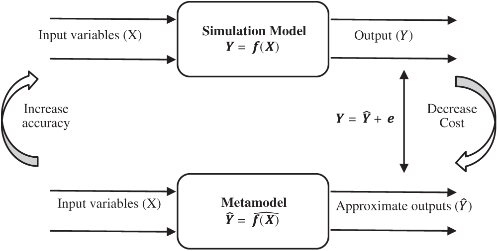
Figure 1: The viewpoint of metamodel and relationship with a simulation model

1.2 Research Contributions

In this study, we develop a new mathematical programming model for the MTPP problem. To solve this mathematical optimization model, we propose a new approach combining the PSO metaheuristic and RBF metamodel applied in the practice of simulation–optimization for wireless signal coverage in the MTPP problem. Among metaheuristic techniques, PSO has attracted wide attention in engineering design problems due to its algorithmic simplicity and powerful search performance [35,36]. Here, we assist the PSO metaheuristic using a radial basis function (RBF) metamodel in an optimization procedure to alleviate the associated computational burden. RBF has become a widely accepted metamodel for deterministic and stochastic simulation metamodeling due to its promising results, particularly in solving complex simulation-based optimization problems [37–40].

The major contributions of our research can be summarized as follows:

     i)  A new mathematical programming model is developed in this paper for coverage optimization in a multi-transmitter placement planning problem. This model has flexibility in the design of optimal placements for any number of transmitters (not limited to an exact number of transmitters in the optimization model).

    ii)  To solve this new optimization model, this paper also proposes a new hybrid technique using a combination of an RBF metamodel and PSO optimizer. The proposed algorithm can search the whole design space continuously with no need to run a simulation model for all investigated locations (thus incurring a low computational cost).

The rest of this paper is organized as follows. Section 2 provides the preliminaries and follows the algorithmic framework of the proposed algorithm which has been developed for the MTPP problem in Section 3. In Section 4, a numerical case study is presented to show the applicability and effectiveness of the proposed algorithm in the simulation–optimization of the MTPP problem. Finally, this paper is concluded in Section 5.

2  Preliminaries

2.1 Radial Basis Function

The RBF is a kind of neural network that employs RBF as a transfer function (see Fig. 2) and consists of an input layer, a hidden radial basis layer, and an output linear layer [41]. The RBF employs a linear combination of independent symmetric functions based on Euclidean distances to compute the approximation function of response.

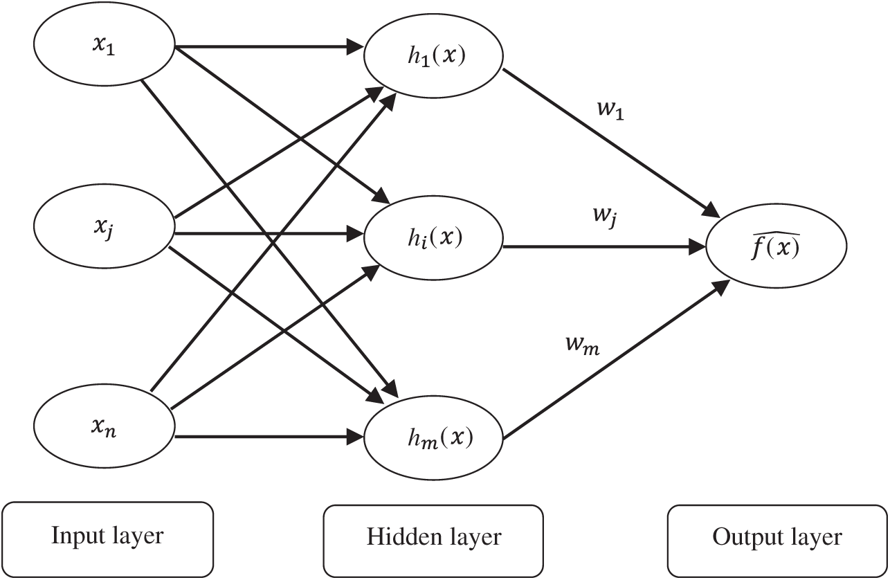
Figure 2: Radial basis function neural network

The simple mathematical forms of RBF can be expressed as

f(x)^=∑i=1mwihi(x)(1)

where wi, (i=1+2+⋯+m) represents the weight coefficients that need to be estimated, m is the number of sample points and hi(x) is the ith radial function. There are different types of RBF, such as linear, cubic, Gaussian, multi-quadratic, and so on [41]. For instance, the common Gaussian form of the radial function is

hi(x)=exp(-ri2)(2)

where ri=∥x-xci∥ is the l2 norm and xci is the center vector of sample point i [42]. The value of the weight parameters wi can be estimated by minimizing the sum square error of model:

MinimizeSSE=∑i=1m(f(xi)-ŷi)2(3)

where f(xi) is the exact output from the original model for the ith sample points and ŷi is related to the predicted output from RBF. As the RBF interpolates the sample points, the SSE is expected to be SSE≈0.

2.2 Particle Swarm Optimization

The canonical PSO algorithm, which simulates the swarm behaviors of social animals, such as bird flocking or fish schooling, was proposed in [43]. The PSO algorithm begins by initializing the population. The second step is the calculation of the fitness values of each particle, followed by updating individual and global bests; later, the velocities and positions of the particles are updated. The second to fourth steps are repeated until the termination condition is satisfied [44,45]. The PSO algorithm is formulated as follows [43–45]:

vidt+1=w*vidt+c1.rand(0,1).(pidt-xidt)+c2.rand(0,1).(pgdt-xidt)andxidt+1=xidt+vidt+1(4)

where w is inertia weight factor, vidt and xidt are the particle velocity and particle position, respectively, d is the dimension in the search space, i is the particle index and t is the iteration number. Expressions c1 and c2 represent the speed, regulating the length when flying towards the most optimal particles of the whole swarm, and the most optimal individual particle. The term pi is the best position achieved so far by particle i, and pg is the best position found by the neighbors of particle i. The expression rand(0,1) represents a random value between 0 and 1. AN exploration happens if either or both of the differences between the particle’s best (pidt) and previous particle’s position (xidt), and between the population’s all-time best (pgdt) and previous particle’s position (xidt) are large, and exploitation occurs when these values are both small. PSO has attracted a great deal of attention in control engineering design problems due to its algorithmic simplicity and powerful search performance [35,36]. However, PSO implementations that require a large number of fitness evaluations before locating the global optimum are often prevented from being applied to computationally expensive real-world problems [46]. Therefore, metamodel-assisted PSO metaheuristic optimization algorithms have attracted great interest in the literature [46–48].

3  Proposed Algorithm

Here, we explain the algorithmic framework of the proposed simulation-based optimization technique based on a hybrid RBF metamodel and PSO metaheuristic. Fig. 3 represents the procedure of the proposed hybrid optimization algorithm in this study along with the construction of the simulation model and analysis of data. Furthermore, the proposed hybrid optimization algorithm is implemented with the following steps:

Input: Simulation of the input/output (I/O) set of data. Here, for the transmitter localization problem, the input data set includes (X, Y) locations, and the output data set includes the average signal coverage (ASC) regarding each location.

Output: Estimation of Pareto frontier including a set of optimal locations for multiple transmitters.

Step 1: Fit RBF metamodel over the I/O data set.

Step 2: Construct the objective function of the optimization model.

Note: In the current paper, in the MTPP problem, we consider the maximization of ASC as an objective function of the model. However, to smooth the amount of signal overlap by transmitters, we control the Euclidean distances between every pair of transmitters in a set of constraints. Let k=1,2,…,K be the number of transmitters in a model; therefore, the proposed optimization model based on a mathematical programming framework is constructed as below:

MaximizeASC=∑k=1KC(Xk,Yk)(5)

Subject to:

d(Ti,Tj)≥β∥h∥Kfor{∀i,j∈(1,2,…,K)|i<j} (6)

0≤Xk≤uX,0≤Yk≤uY (7)

where Ck(X,Y) is the RBF estimation of ASC in location (X, Y) for the kth transmitter. The terms uX and uY indicate the length and width of the design space. The expression d(Ti,Tj)=d(Tj,Ti)={(Xi-Xj)2+(Yi-Yj)2}12 shows the Euclidean distance (norm) between two locations of the ith and jth transmitters. The expression ∥h∥ shows the maximum Euclidean distance between two locations in the design space. The weight scale β is defined by the decision-maker and indicates the emphasis of the model over the distances between transmitters to smooth the overall signal coverage. From Eq. (5) the optimal result depends on the value of β, which can be chosen by the decision-maker. Varying β allows the capture of the Pareto frontier (also called Pareto optimal efficiency). The set of optimal solutions obtained by fluctuating β in the model provides an estimate of the Pareto frontier [49]. As the aforementioned mathematical model is constrained (see Eq. (6)), a constraint handling method should be integrated into the optimization algorithm. There are several methods for handling constraints in the literature, such as penalty functions, special operators, repair algorithms, the separation of objectives and constraints, and hybrid methods [50]. In this study, we use the simplest method, called the death penalty. In this method, search agents that violate any of the constraints at any level are treated as the same and penalized by assigning a large fitness value (small objective value in case of maximization). This method is very cheap and readily applicable to the PSO algorithm without algorithm modifications [50,51].

Step 3: Run the PSO optimizer for the constructed optimization model in the previous step and obtain the optimal result.

Step 4: Repeat the three previous steps for different values of β in Eq. (6) to obtain the estimation of the Pareto frontier.

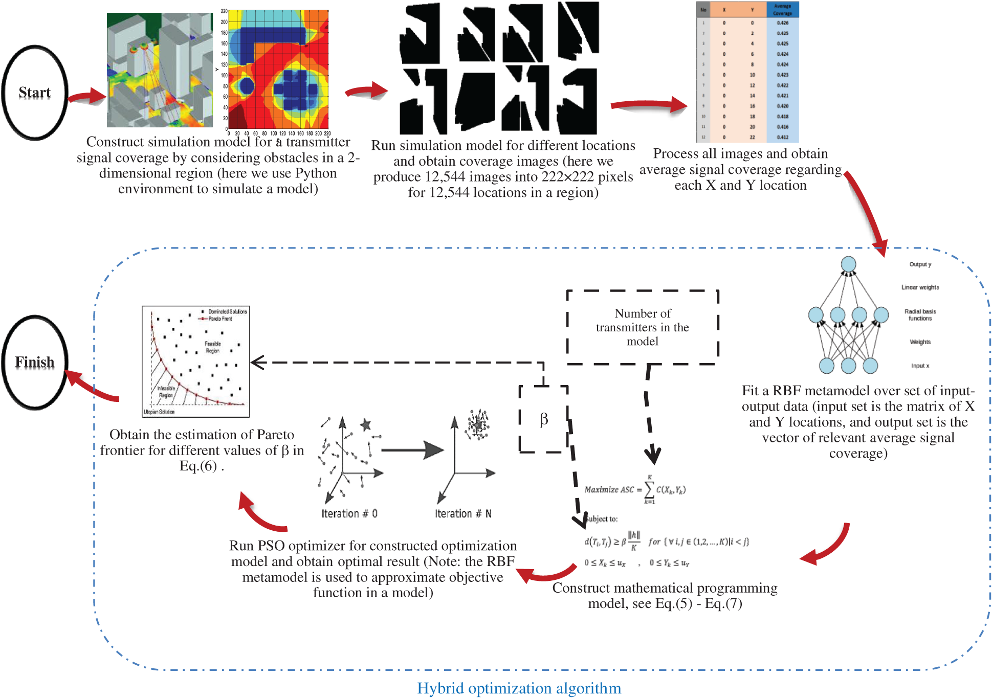
Figure 3: The simulation-based optimization method in the current study including the procedure of proposed hybrid RBF/PSO algorithm in conjunction with simulation model and data analyzing

4  Simulation-Based Optimization of MTPP: Case Study

In this section, the applicability of the proposed algorithm in the MTPP problem is studied to obtain the optimal locations of each transmitter to maximize the amount of signal coverage. To continue, first, the application of the proposed algorithm using the hybrid RBF metamodel and PSO metaheuristic integrated by mathematical programming in the current MTPP optimization problem is explained; then, the obtained results are discussed in detail.

4.1 Simulation Setup

In this work, we used a ray-tracing simulator developed in Python. We created a simulation model that simulated the environment of an office room to implement the MTPP problem. The obstacles in the room were modeled according to the layout of the office equipment by creating a polygon of each object and placing it in various positions in the room. The calculations of the coverage area assumed that the signal propagation was omnidirectional, and the transmitter could transmit the signal in two dimensions. To evaluate the coverage rate in a two-dimensional area, we divided the entire monitoring region into 222×222 pixels. We applied the binary model in this study, meaning set 0 for the area that the transmitter did not cover and 1 for the area that the transmitter successfully covered.

To reduce the number of simulation runs and produced images, we decussated odd locations (odd X and Y positions) in the two-dimension design area to set the transmitter; thus, only coverage images were produced for even pixels, meaning that we produced 12,544 images. Then, we analyzed the set of images gained from the simulation model to obtain the ASC for each relevant X and Y location (i.e., in the following, this computed dataset is used as the set of I/O data for the optimization procedure). We used the Matlab® environment to analyze the data set. However, 12,544 sets of input (X and Y locations) and output data (ASC regarding each location) were produced. We used the Matlab® “Deep learning” toolbox to construct the RBF metamodel and applied the “particle swarm optimization” toolbox to perform PSO global optimization. We defined both the X axis and Y axis in the same range of [0, 222]. Fig. 4 shows the scatter plot for 12,544 different (X, Y) locations and the relevant average coverages for one transmitter. Notably, in the current simulation model, we assumed zero coverage for areas with obstacles in the design space. Fig. 5 illustrates the contour plot of signal coverage in two-dimensions of the design space including the obstacle areas with zero coverage (areas with dark blue color). From the initial simulation model, by locating one transmitter, the maximum ASC was obtained in a location of X = 26 and Y = 0 with ASC = 0.4355 (see Fig. 6).

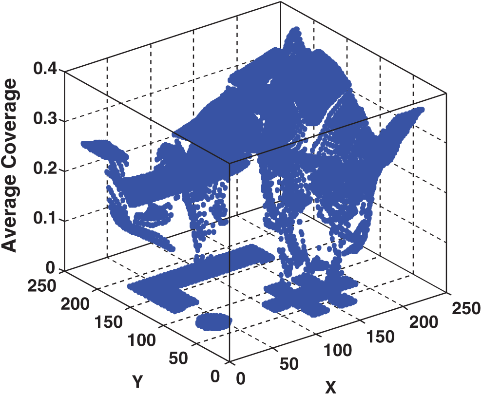
Figure 4: Three-dimensions scatter plot for different (X, Y) transmitter locations and relevant average signal coverage

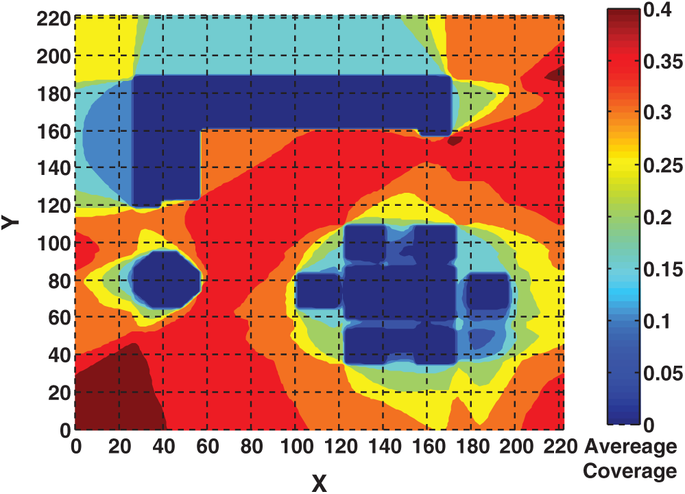
Figure 5: Contour plot for average coverage using one transmitter in all locations of design space. Obstacles areas show in dark blue color with zero signal coverage

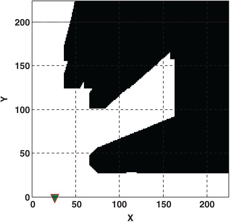
Figure 6: Maximum signal coverage in the model with one transmitter is obtained in X = 26, Y = 0 with ASC = 0.4355. Black areas include obstacles and not covered by transmitter

This work aimed to develop a new method to investigate the optimal locations of multiple transmitters. However, in the current instance, we applied the proposed algorithm. Note that the proposed algorithm is flexible for any number of transmitters, and we are not limited to the number of transmitters in a model. Here, to show the applicability and effectiveness of the proposed algorithm, the MTPP problem was investigated for two, three, four, and five transmitters, respectively. For this purpose, we first constructed the RBF metamodel over the set of I/O data obtained from the simulation model. We used the “newrbe” Matlab® function to construct the RBF metamodel. Fig. 7 shows the surface plot of the constructed RBF metamodel and scatter plot of the relevant mean square error of prediction.

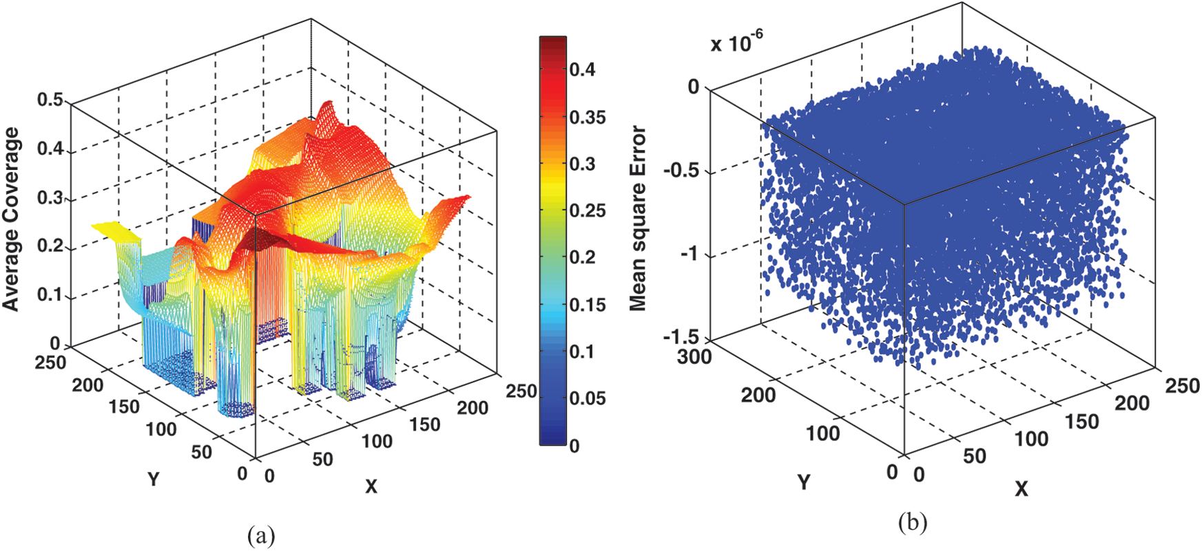
Figure 7: Surface plot of fitted RBF metamodel (a) and scatter plot for mean square error of constructed RBF prediction (b)

4.2 Mathematical Formulations

We constructed the mathematical programming model for the MTPP problem (see Eq. (5) till Eq. (7)) with two, three, four, and five transmitters (K = 2, 3, 4, 5) in a model, respectively. The design ranges for both the X axis and Y axis were 0≤Xk≤222 and 0≤Yk≤222, respectively. ∥h∥ is the maximum distance between two locations, which here is the square diameter in the design space and equal to ∥h∥={(222-0)2+(222-0)2}12=313.956. We repeated the optimization model for K = 2, 3, 4, 5 three times for β=0.5, β=1, and β=1.5 (see Eq. (6)). However, we ran the PSO optimizer for each optimization model, respectively. As we used the RBF metamodel instead of the original simulation model, we did not consider the number of function evaluations (iterations) required by the PSO global optimizer. In the following, we first sketch the mathematical programming model for each MTPP problem with two, three, four, and five transmitters (K = 2, 3, 4, 5), respectively.

Objective function:

MaximizeASC=∑k=1Krbf(Xk,Yk),fork=1,2,…,K(8)

Constraints:

di,j≥β(313.9562),for{∀i,j∈(1,2,…,K)|i<j}0≤Xk≤222,0≤Yk≤222fork=1,2,…,K(9)

where di, j shows the Euclidean distance between transmitters (e.g., d1,2={(X1−X2)2+ (Y1−Y2)2}12), indicating the distance between the first and second transmitters in the design space. Besides, rbf(X.,Y.) shows the RBF metamodel that previously was fitted over 12,544 I/O data sets obtained from the simulation model (X and Y locations as a two-dimensional input set and the ASC for each location as an output set). Below, the obtained results for the MTPP optimization problems are discussed.

4.3 Results

In the model with two transmitters (K = 2), we applied the proposed algorithm by integrating the RBF metamodel constructed over a set of I/O data (i.e., I/O data obtained from the simulation model) and PSO optimizer. The optimization results in the model with two transmitters for three different values of β (see Eq. (6)) are shown in Tab. 1. Fig. 8 provides the schematic signal coverage in the design space when two transmitters are located on their computed optimal locations. This figure shows the schematic image for signal coverage in the design space (222×222 pixels) for problems with two transmitters for three different values of β, respectively when the transmitters are located optimally on their computed optimal locations using the proposed algorithm. White zones in these images show the area covered by the signal, while black zones (mostly obstacles) show areas that were not covered by the signal of the transmitters. The optimal locations of transmitters are also shown in each image. The proposed algorithm aims to maximize the average signal coverage for each problem. As can be seen, the highest ASC was obtained by a β=0.5 equal to 0.733. The optimization procedures for both β=1 and β=1.5 provided the same results (the same locations for two transmitters) with ASC = 0.713.

Table 1: The optimal locations and relevant overall signal coverage for two-transmitters localization model

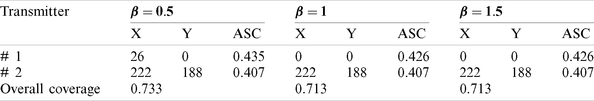
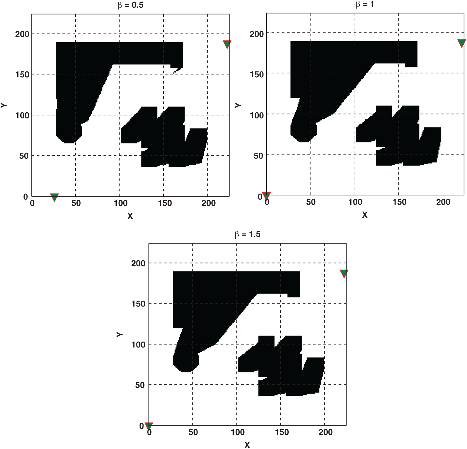
Figure 8: Optimal locations (i.e., are shown by triangle marker) and overall signal coverage of two transmitters in MTL problem for β=0.5, β=1, and β=1.5. Black areas include obstacles and not covered by transmitters

Next, we constructed the optimization procedure based on the proposed hybrid RBF and PSO algorithm for a case with three transmitters in the model. The obtained optimization results are shown in Tab. 2 for three different β values, and schematic coverages for the optimal locations of transmitters are illustrated in Fig. 9. The optimal locations of transmitters and areas covered by the signal from the transmitters are shown in each image. The black zones (mostly obstacles) show areas that were not covered by the signal from the transmitters. As can be seen from Tab. 2, the highest signal coverage was obtained for β=0.5 and β=1 by ASC = 0.746 when three transmitters were optimally located in the design space. With the same procedure, the proposed optimization algorithm was used for the model with four transmitters, and the obtained results are depicted in Tab. 3 and Fig. 10. For a case with four transmitters, the highest signal coverage in the model was obtained by ASC = 0.802 in β=1, followed closely by β=0.5 with ASC = 0.794.

Table 2: The optimal locations and relevant overall signal coverage for three-transmitters localization model

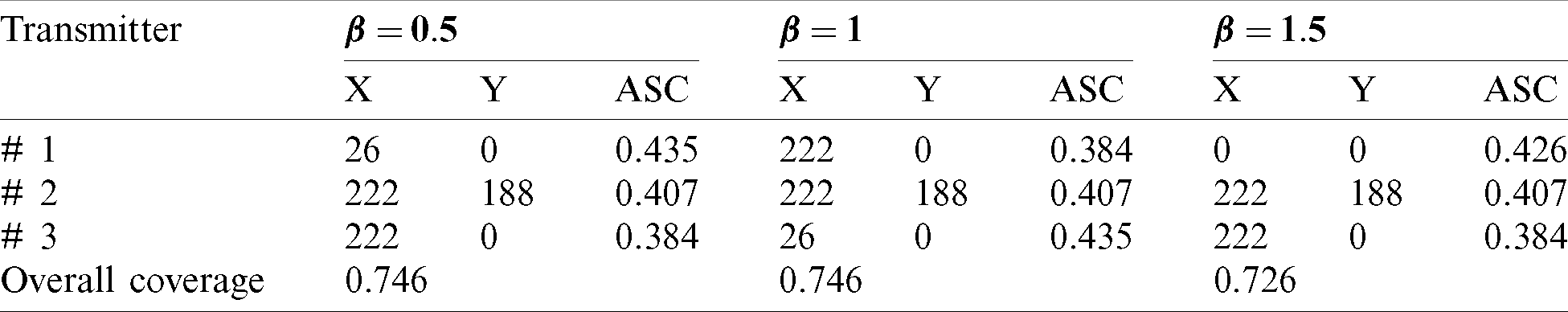
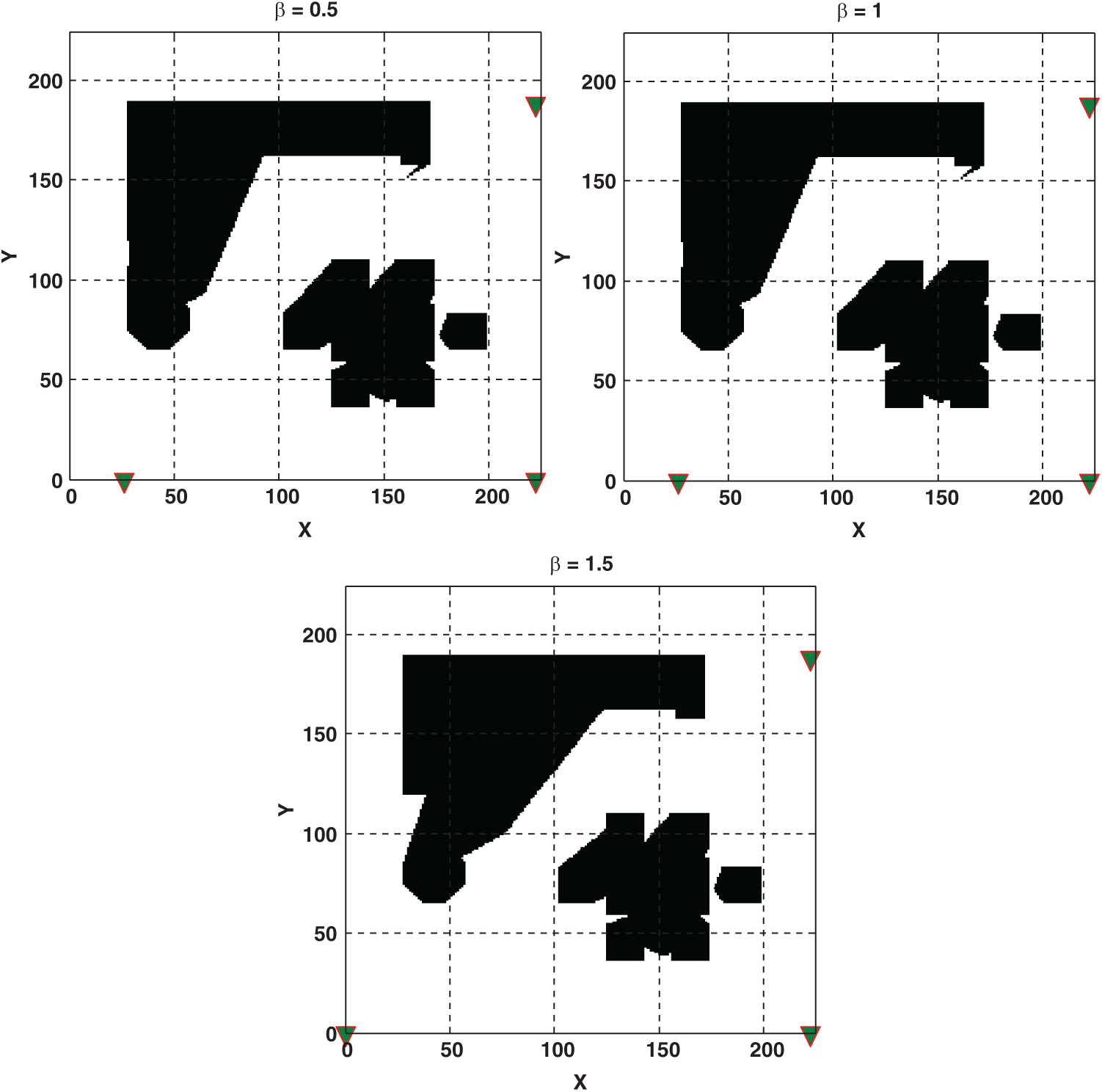
Figure 9: Optimal locations (i.e., are shown by triangle marker) and overall signal coverage of three transmitters in MTL problem for β=0.5, β=1, and β=1.5. Black areas include obstacles and not covered by transmitters

Table 3: The optimal locations and relevant overall signal coverage for four-transmitters localization model

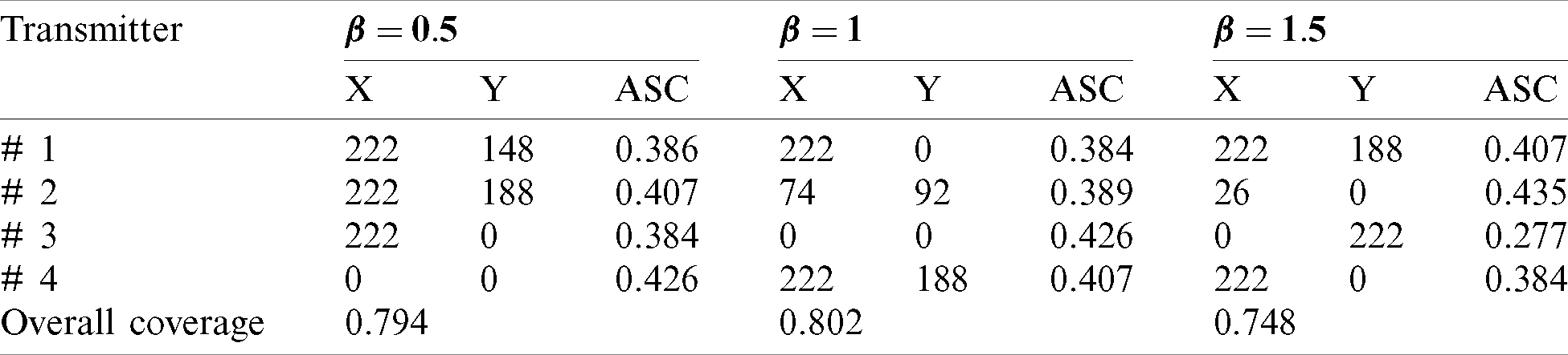
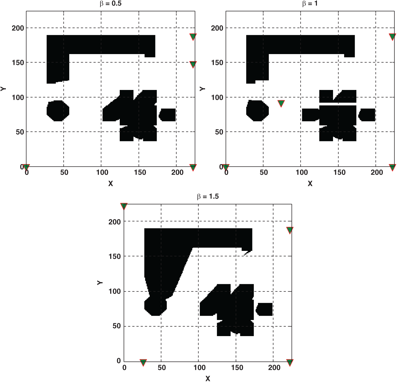
Figure 10: Optimal locations (i.e., are shown by triangle marker) and overall signal coverage of four transmitters in MTL problem for β=0.5, β=1, and β=1.5. Black areas include obstacles and not covered by transmitters

Besides, the application of the proposed algorithm was used for the MTPP problem with five transmitters. Optimal locations and relevant obtained results are provided in Tab. 4 and schematically are shown in Fig. 11. The obtained results for the optimization of a model with five transmitters revealed that the highest signal coverage was obtained in β=1 by ASC = 0.802, which was the same as the model with four transmitters.

Table 4: The optimal locations and relevant overall signal coverage for five-transmitters localization model

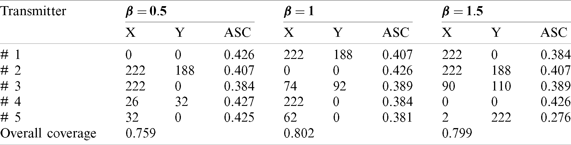
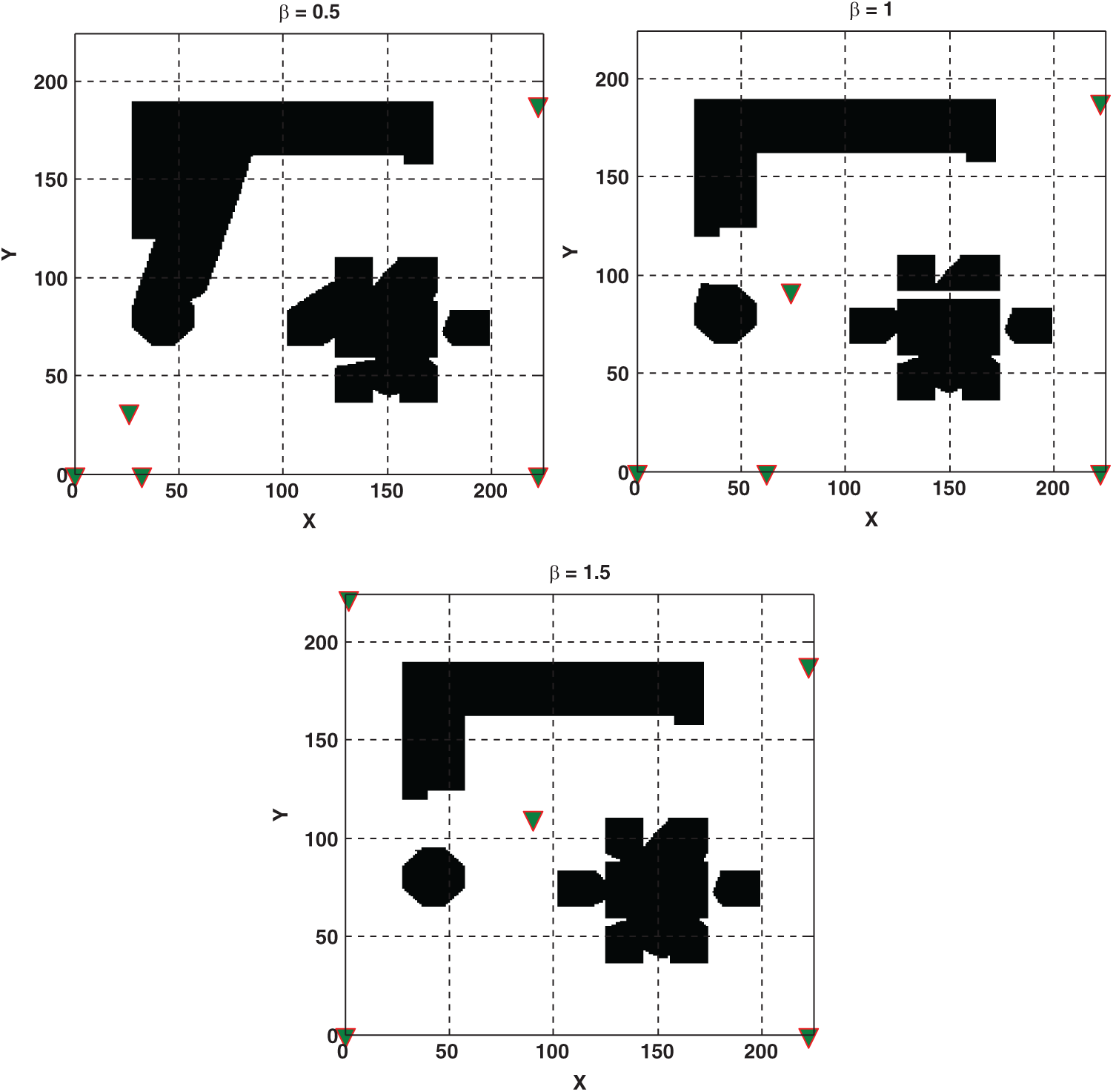
Figure 11: Optimal locations (i.e., are shown by triangle marker) and overall signal coverage of five transmitters in MTL problem for β=0.5, β=1, and β=1.5. Black areas include obstacles and not covered by transmitters

Finally, we compared all obtained results based on β=0.5, β=1, and β=1.5, as shown in Fig. 12. β=0.5 shows good results for the models with two, three, and four transmitters but not for the model with five transmitters. However, due to the considered obstacle areas in the original simulation model, the model with five transmitters exhibited very similar behavior in terms of the covering design space with the model using four transmitters. Thus, it is not cost-effective to use a higher number of transmitters when almost maximum signal coverage can be obtained with four transmitters.

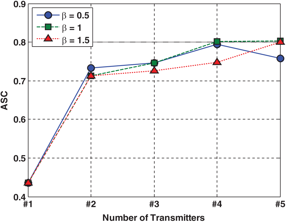
Figure 12: Average signal coverage for different number of transmitters in the model based on three different β values

4.4 Discussion

Here, we developed a new mathematical programming model for the MTPP problem. This model has flexibility in terms of the design of optimal placements for any number of transmitters (not limited to an exact number of transmitters in the optimization model). To solve this new optimization model, we also propose a new hybrid technique using a combination of the RBF metamodel and PSO optimizer. In comparison with common model-based optimization techniques, two main advantages of the proposed hybrid algorithm are as follows:

     i)  The proposed algorithm can search in the whole design space continuously. In other words, in the current instance in this paper, we are not restricted to investigating optimal locations only by discrete areas when searching among the 12,544 locations (as aforementioned, the signal coverage for 12,544 locations in the two-dimensional design space is modeled and computed through the simulation model); thus, any area within these 12,544 locations can be investigated as well because we APPLY the interpolation method (the well-known RBF metamodel) that can be trained on the whole design space. In contrast, the model-based optimization techniques are limited to searching only within a limited number of locations.

    ii)  In the current paper, for the MTPP problem, one way to tackle the previous shortcomings in the case of using model-based techniques for coverage optimization is that the number of locations modeled in the simulation can be increased. However, the simulation model needs to run with a larger number of locations (more than 12,544 locations in the current study) and compute the signal coverage for locations with smaller distances. However, this procedure can increase the computational cost of optimization significantly.

There are two main limitations in the current study, as stated below:

     i)  The proposed method employs the RBF metamodel to train the black-box simulation model. Therefore, the approximate errors cannot be ignored when solving inequality-constrained simulation-based optimization problems. A challenge for optimization under restricted budgets (limited number of sample points) will be to find the right degree of approximation (smoothing factor) from only a relatively few samples [52]. Other metamodels, such as Kriging, polynomial regression, and neural networks, can be used and compared with the RBF metamodel used in the current study for the MTPP problem.

    ii)  In this study, we use the common death penalty method to deal with inequality constraints in the optimization model. However, other constraint handling methods [50] can be used and compared with the results of this study.

5  Conclusions

Simulation-based optimization is a viable solution for solving complex real-world problems, such as the base station placement problem in wireless sensor networks. The multi-transmitter placement planning problem of guaranteeing coverage while meeting some application requirements quite often gives rise to NP-hard optimization problems. In this paper, we developed a new mathematical programming model to handle the design of optimal locations for any number of transmitters in a two-dimensional design space. To solve the mentioned MTPP model, we proposed a new hybrid method combining the PSO metaheuristic and RBF metamodel. The applicability of the proposed method was shown using a simulation-based MTPP optimization problem with two, three, four, and five transmitters. The results showed the effectiveness of the proposed algorithm for solving a mathematical model of the MTPP optimization problem with a computationally less expensive method. The results also showed that, in the current case study, cost-effective signal coverage concerning considered obstacles could be obtained with four transmitters (with an average signal coverage equal to 82% of the area in the model), and more transmitters did not provide a significant change in the amount of average signal coverage. This approach can continuously search the whole of the design space to obtain optimal locations for any number of transmitters in the model without requiring the simulation of signal coverage for all locations via a simulation model. The RBF metamodel can train the model using a black-box simulation model and a limited amount of input-output data to approximate all locations in the design space. Finally, the limitations of the current study were discussed. Regarding the mentioned limitations of the current study, future research can be addressed.

Funding Statement: This research project is funded by TSRI Fund (CU_FRB640001_01_21_6). Amir Parnianifard would like to acknowledge the financial support by Second Century Fund (C2F), Chulalongkorn University, Bangkok. Sattam Al Otaibi would like to thank Taif University Researchers Supporting Project number (TURSP-2020/228), Taif University, Taif, Saudi Arabia for the financial support.

Conflicts of Interest: The authors declare that they have no conflicts of interest to report regarding the present study.

References

 1.  E. Waleed, S. Kandeepan and A. Anpalagan. (2015). “Optimal placement and number of energy transmitters in wireless sensor networks for RF energy transfer,” in IEEE 26th Annual Int. Symp. on Personal, Indoor, and Mobile Radio Communications, Hong Kong, pp. 1238–1243. [Google Scholar]

 2.  A. Fahad, N. Lasla and M. Younis. (2016). “Coverage-based node placement optimization in wireless sensor network with linear topology,” in IEEE Int. Conf. on Communications, Kuala Lumpur, Malaysia, pp. 1–6. [Google Scholar]

 3.  M. Saadi, M. T. Noor, A. Imran, W. T. Toor, S. Mumtaz et al. (2020). , “IoT enabled quality of experience measurement for next generation networks in smart cities,” Sustainable Cities and Society, vol. 60, no. 9, pp. 102266. [Google Scholar]

 4.  C. B. Mwakwata, H. Malik, M. Alam, L. Moullec, S. Parand et al. (2019). , “Narrowband internet of things (NB-IoTFrom physical (PHY) and media access control (MAC) layers perspectives,” Sensors, vol. 19, no. 11, pp. 2613. [Google Scholar]

 5.  M. S. Omar, S. A. Hassan, H. Pervaiz, Q. Ni, L. Musavian et al. (2017). , “Multiobjective optimization in 5G hybrid networks,” IEEE Internet of Things Journal, vol. 5, no. 3, pp. 1588–1159. [Google Scholar]

 6.  Z. Miao, X. Yuan, F. Zhou, X. Qiu, Y. Song et al. (2020). , “Grey wolf optimizer with an enhanced hierarchy and its application to the wireless sensor network coverage optimization problem,” Applied Soft Computing, vol. 96, no. 3, pp. 106602. [Google Scholar]

 7.  S. Wang, X. Yang, X. Wang and Z. Qian. (2019). “A virtual force algorithm-Lévy-embedded grey wolf optimization algorithm for wireless sensor network coverage optimization,” Sensors, vol. 19, no. 12, pp. 2735. [Google Scholar]

 8.  A. Gogu, D. Nace, A. Dilo and N. Mertnia. (2011). “Optimization problems in wireless sensor networks,” in IEEE Int. Conf. on Complex, Intelligent, and Software Intensive Systems, Washington, United States, pp. 302–309. [Google Scholar]

 9.  W. H. Liao, Y. Kao and R. T. Wu. (2011). “Ant colony optimization based sensor deployment protocol for wireless sensor networks,” Expert Systems with Applications, vol. 38, no. 6, pp. 6599–6605. [Google Scholar]

10. S. Fidanova, P. Marinov and E. Alba. (2010). “ACO for optimal sensor layout,” in IJCCI (ICECValencia, Spain, pp. 5–9. [Google Scholar]

11. S. Okdem and D. Karaboga. (2010). “Routing in wireless sensor networks using an ant colony optimization (ACO) router chip,” Sensors, vol. 9, no. 2, pp. 909–921. [Google Scholar]

12. K. Saleem, N. Fisal, M. A. Baharudin, A. A. Ahmed, S. Hafizah et al. (2010). , “Ant colony inspired self-optimized routing protocol based on cross layer architecture for wireless sensor networks,” WSEAS Transactions on Communications, vol. 9, no. 10, pp. 669–678. [Google Scholar]

13. M. Xiao, S. Mumtaz, Y. Huang, L. Dai, Y. Li et al. (2017). , “Millimeter wave communications for future mobile networks (guest editorialPart I,” IEEE Journal on Selected Areas in Communications, vol. 35, no. 7, pp. 1425–1431. [Google Scholar]

14. N. A. B. Aziz, A. W. Mohemmed and M. Y. Alias. (2009). “A wireless sensor network coverage optimization algorithm based on particle swarm optimization and Voronoi diagram,” in IEEE Int. Conf. on Networking, Sensing and Control, Okayama, Japan, pp. 602–607. [Google Scholar]

15. W. T. Liu and Z. Y. Fan. (2011). “Coverage optimization of wireless sensor networks based on chaos particle swarm algorithm,” Journal of Computer Applications, vol. 2, no. 2, pp. 338–340. [Google Scholar]

16. W. W. Ismail and S. A. Manaf. (2010). “Study on coverage in wireless sensor network using grid based strategy and particle swarm optimization,” in IEEE Asia Pacific Conf. on Circuits and Systems, Kuala Lumpur, Malaysia, pp. 1175–1178. [Google Scholar]

17. Y. Liu, X. Fang, M. Xiao and S. Mumtaz. (2018). “Decentralized beam pair selection in multi-beam millimeter-wave networks,” IEEE Transactions on Communications, vol. 66, no. 6, pp. 2722–2737. [Google Scholar]

18. A. Parnianifard, A. S. Azfanizam, M. K. A. Ariffin and M. I. S. Ismail. (2020). “Comparative study of metamodeling and sampling design for expensive and semi-expensive simulation models under uncertainty,” Simulation, vol. 96, no. 1, pp. 89–110. [Google Scholar]

19. G. G. Wang and S. Shan. (2007). “Review of metamodeling techniques in support of engineering design optimization,” Journal of Mechanical Design, vol. 129, no. 4, pp. 370–380. [Google Scholar]

20. T. W. Simpson, J. D. Poplinski, P. N. Koch and J. K. Allen. (2001). “Metamodels for computer-based engineering design: Survey and recommendations,” Engineering with Computers, vol. 17, no. 2, pp. 129–150. [Google Scholar]

21. M. Umer, L. Kulik and E. Tanin. (2008). “Kriging for localized spatial interpolation in sensor networks,” in Int. Conf. on Scientific and Statistical Database Management, Hong Kong. [Google Scholar]

22. A. Parnianifard, A. S. Azfanizam, M. K. A. Ariffin and M. I. S. Ismail. (2018). “Kriging-Assisted robust black-box simulation optimization in direct speed control of DC motor under uncertainty,” IEEE Transactions on Magnetics, vol. 54, no. 7, pp. 1–10. [Google Scholar]

23. A. Parnianifard, M. Fakhfakh, M. Kotti, A. Zemouche and L. Wuttisittikulkij. (2020). “Robust tuning and sensitivity analysis of stochastic integer and fractional-order PID control systems: Application of surrogate-based robust simulation-optimization,” International Journal of Numerical Modelling: Electronic Networks, Devices and Fields, vol. 34, no. 2, pp. 556. [Google Scholar]

24. A. Parnianifard, A. Zemouche, R. Chancharoen, M. A. Imran and L. Wuttisittikulkij. (2020). “Robust optimal design of FOPID controller for five bar linkage robot in a Cyber-Physical System: A new simulation-optimization approach,” PLoS One, vol. 15, no. 11, pp. e0242613. [Google Scholar]

25. J. Havinga and G. Klaseboer. (2017). “Sequential improvement for robust optimization using an uncertainty measure for radial basis functions,” Structural and Multidisciplinary Optimization, vol. 55, no. 4, pp. 1345–1363. [Google Scholar]

26. X. Liu, C. Ma, M. Li and M. Xu. (2011). “A kriging assisted direct torque control of brushless DC motor for electric vehicles,” IEEE Seventh Int. Conf. on Natural Computation, vol. 3, pp. 1705–1710. [Google Scholar]

27. A. Parnianifard and A. Azfanizam. (2020). “Metamodel-based robust simulation-optimization assisted optimal design of multiloop integer and fractional-order PID controller,” International Journal of Numerical Modelling: Electronic Networks, Devices and Fields, vol. 33, no. 1, pp. 1. [Google Scholar]

28. X. Liu, M. Li and M. Xu. (2016). “Kriging assisted on-line torque calculation for brushless DC motors used in electric vehicles,” International Journal of Automotive Technology, vol. 17, no. 1, pp. 153–164. [Google Scholar]

29. G. Liu, B. Xu and H. Chen. (2014). “An indicator kriging method for distributed estimation in wireless sensor networks,” International Journal of Communication Systems, vol. 27, no. 1, pp. 68–80. [Google Scholar]

30. M. Saadi, Z. Saeed, T. Ahmad, M. K. Saleem, L. Wuttisittikulkij et al. (2019). , “Visible light-based indoor localization using k-means clustering and linear regression,” Transactions on Emerging Telecommunications Technologies, vol. 30, no. 2, pp. e3480. [Google Scholar]

31. Z. Yang, M. R. Chen and W. Wu. (2014). “Algorithm for wireless sensor network data fusion based on radial basis function neural networks,” Applied Mechanics and Materials, vol. 577, pp. 873–878. [Google Scholar]

32. Z. Zhou, H. Yu, C. Xu, Z. Chang, S. Mumtaz et al. (2018). , “BEGIN: Big data enabled energy-efficient vehicular edge computing,” IEEE Communications Magazine, vol. 56, no. 12, pp. 82–89. [Google Scholar]

33. S. Y. M. Vaghefi and R. M. Vaghefi. (2011). “A novel multilayer neural network model for TOA-based localization in wireless sensor networks,” in IEEE Int. Joint Conf. on Neural Networks, San Jose, CA, USA, pp. 3079–3084. [Google Scholar]

34. A. Payal, C. S. Rai and B. V. R. Reddy. (2014). “Analysis of radial basis function network for localization framework in wireless sensor networks,” in EEE 5th Int. Conf.-Confluence The Next Generation Information Technology Summit, Noida, India, pp. 432–435. [Google Scholar]

35. M. P. Aghababa. (2016). “Optimal design of fractional-order PID controller for five bar linkage robot using a new particle swarm optimization algorithm,” Soft Computing, vol. 20, no. 10, pp. 4055–4067. [Google Scholar]

36. M. Zamani, M. Karimi-Ghartemani, N. Sadati and M. Parniani. (2009). “Design of a fractional order PID controller for an AVR using particle swarm optimization,” Control Engineering Practice, vol. 17, no. 12, pp. 1380–1387. [Google Scholar]

37. D. J. Fonseca, D. O. Navaresse and G. P. Moynihan. (2003). “Simulation metamodeling through artificial neural networks,” Engineering Applications of Artificial Intelligence, vol. 16, no. 3, pp. 177–183. [Google Scholar]

38. R. A. Kilmer, A. E. Smith and L. J. Shuman. (1999). “Computing confidence intervals for stochastic simulation using neural network metamodels,” Computers & Industrial Engineering, vol. 36, no. 2, pp. 391–407. [Google Scholar]

39. M. Scardi. (2001). “Advances in neural network modeling of phytoplankton primary production,” Ecological Modelling, vol. 146, no. 1–3, pp. 33–45. [Google Scholar]

40. F. M. Alam, K. R. McNaught and T. J. Ringrose. (2004). “A comparison of experimental designs in the development of a neural network simulation metamodel,” Simulation Modelling Practice and Theory, vol. 12, no. 7, 8, pp. 559–578. [Google Scholar]

41. M. D. Buhmann. (2003). Radial Basis Functions: Theory and Implementations, Cambridge, England: Cambridge University Press. [Google Scholar]

42. C. S. K. Dash, A. K. Behera, S. Dehuri and S. B. Cho. (2016). “Radial basis function neural networks: A topical state-of-the-art survey,” Open Computer Science, vol. 1, pp. 33–63. [Google Scholar]

43. J. Kennedy and R. Eberhart. (1995). “Particle swarm optimization,” Proc. of ICNN’95-Int. Conf. on Neural Networks, vol. 4, pp. 1942–1948. [Google Scholar]

44. M. N. Ab-Wahab, S. Nefti-Meziani and A. Atyabi. (2015). “A comprehensive review of swarm optimization algorithms,” PLoS One, vol. 10, no. 5, pp. e0122827. [Google Scholar]

45. Y. D. Valle, G. L. Venayagamoorthy, S. Mohagheghi, J. C. Hernandez and R. G. Harley. (2008). “Particle swarm optimization: Basic concepts, variants and applications in power systems,” IEEE Transactions on Evolutionary Computation, vol. 12, no. 2, pp. 171–195. [Google Scholar]

46. H. Yu, Y. Tan, J. Zeng, C. Sun and Y. Jin. (2018). “Surrogate-assisted hierarchical particle swarm optimization,” Information Sciences, vol. 454, pp. 59–72. [Google Scholar]

47. S. Dutta. (2020). “A sequential metamodel-based method for structural optimization under uncertainty,” Structures, vol. 26, no. 5, 6, pp. 54–65. [Google Scholar]

48. R. G. Regis. (2014). “Particle swarm with radial basis function surrogates for expensive black-box optimization,” Journal of Computational Science, vol. 5, no. 1, pp. 12–23. [Google Scholar]

49. K. Miettinen. (2012). Nonlinear Multiobjective Optimization, Vol. 12. Berlin, Germany: Springer Science & Business Media. [Google Scholar]

50. C. A. C. Coello. (2002). “Theoretical and numerical constraint-handling techniques used with evolutionary algorithms: A survey of the state of the art,” Computer Methods in Applied Mechanics and Engineering, vol. 191, no. 11, 12, pp. 1245–1287. [Google Scholar]

51. S. Mirjalili. (2015). “The ant lion optimizer,” Advances in Engineering Software, vol. 83, pp. 80–98. [Google Scholar]

52. S. Bagheri, W. Konen, M. Emmerich and T. Bäck. (2017). “Self-adjusting parameter control for surrogate-assisted constrained optimization under limited budgets,” Applied Soft Computing, vol. 61, no. 6, pp. 377–393. [Google Scholar]

This work is licensed under a Creative Commons Attribution 4.0 International License, which permits unrestricted use, distribution, and reproduction in any medium, provided the original work is properly cited.