Computers, Materials & Continua DOI:10.32604/cmc.2021.015514
Article

Optimum Location of Field Hospitals for COVID-19: A Nonlinear Binary Metaheuristic Algorithm

Said Ali Hassan1, Khalid Alnowibet2, Prachi Agrawal3 and Ali Wagdy Mohamed4,5,*

1Department of Operations Research and Decision Support, Faculty of Computers and Artificial Intelligence, Cairo University, Giza, 12613, Egypt
2College of Science, Department of Statistics and Operations Research, King Saud University, Riyadh, Saudi Arabia
3Department of Mathematics and Scientific Computing, National Institute of Technology Hamirpur, Himachal Pradesh, 177005, India
4Department of Operations Research, Faculty of Graduate Studies for Statistical Research, Cairo University, Giza, 12613, Egypt
5Wireless Intelligent Networks Center (WINC), School of Engineering and Applied Sciences, Nile University, Giza, Egypt
*Corresponding Author: Ali Wagdy Mohamed. Email: aliwagdy@gmail.com
Received: 25 November 2020; Accepted: 02 February 2021

Abstract: Determining the optimum location of facilities is critical in many fields, particularly in healthcare. This study proposes the application of a suitable location model for field hospitals during the novel coronavirus 2019 (COVID-19) pandemic. The used model is the most appropriate among the three most common location models utilized to solve healthcare problems (the set covering model, the maximal covering model, and the P-median model). The proposed nonlinear binary constrained model is a slight modification of the maximal covering model with a set of nonlinear constraints. The model is used to determine the optimum location of field hospitals for COVID-19 risk reduction. The designed mathematical model and the solution method are used to deploy field hospitals in eight governorates in Upper Egypt. In this case study, a discrete binary gaining–sharing knowledge-based optimization (DBGSK) algorithm is proposed. The DBGSK algorithm is based on how humans acquire and share knowledge throughout their life. The DBGSK algorithm mainly depends on two junior and senior binary stages. These two stages enable DBGSK to explore and exploit the search space efficiently and effectively, and thus it can solve problems in binary space.

Keywords: Facility location; nonlinear binary model; field hospitals for COVID-19; gaining–sharing knowledge-based metaheuristic algorithm

1  Introduction

Countries all over the world are working tirelessly to find new and better methods to face and defeat the novel coronavirus 2019 (COVID-19). Reference [1] shows that the number of infections is significantly increasing, and hospitals are overcrowded with patients. Many countries have resorted to the only known solution left: The construction of field hospitals. These hospitals are established to meet the needs of treating new coronavirus cases. References [2,3] state that many countries that are recorded to have the highest numbers of COVID-19 cases, such as China, United States, Spain, and France, have built field hospitals. Field hospitals are temporary medical units that are established to take care of and treat patients according to the approved treatment protocols in times of natural disasters, crisis, or pandemics. They also help in relieving the load put on the countries’ existing public and private hospitals.

It is of great importance to place field hospitals geographically close to the places most vulnerable to infection by COVID-19, and to serve the largest number of patients who need healthcare under the constraints of limited available resources. The location of facilities is particularly critical where the implications of poor location decisions extend well beyond cost and patient service considerations. If too few facilities are utilized and/or they are not well located, mortality and morbidity rates can increase. Thus, facility location modeling takes on even greater importance when applied to the setting of healthcare facilities. Reference [4] discusses eight basic facility location models: Set covering, maximal covering, P-center, P-dispersion, P-median, fixed charge, hub, and maxi sum. In all these models, the underlying network is given, as are the demand locations to be served by all facilities and the locations of existing facilities (if pertinent). The general problem is to locate new facilities to optimize some objective like distance or some measure functionally related to distance (e.g., travel time, cost, and/or demand satisfaction). This is fundamental, and thus problems are classified according to their consideration of distance. The first four basic facility location models are based on maximum distance, and the last four are based on total (or average) distance.

Reference [5] states that a priori maximum distances are known as “covering” distances in the facility location models based on maximum distance, and demand within the covering distance to its closest facility is considered “covered.” Meanwhile, reference [4] shows that many facility location planning situations are concerned with the total travelled distance between facilities and demand nodes.

Three classic facility location models are the basis for almost all facility location models that are used in healthcare applications. These are the set covering model, the maximal covering model, and the P-median model.

It is very important to note that location models are application-specific; that is, their structural form (the objectives, constraints, and variables) is determined by the particular location problem under study. Consequently, no general location model appropriate for all current or potential applications exists.

In this paper, a modified version of the maximal covering model is designed to be suitable for the optimum location of healthcare field hospitals for COVID-19. This designed model is a nonlinear binary mathematical programming model.

The structure of this paper is as follows. The first section presents an introduction and contains a concise point content for each subsequent section in this article. The second section presents a brief review of the three basic facility location models that are the most suitable for application in the healthcare field: The set covering model, the maximal covering model, and the P-median model. Section 3 introduces the location of field hospitals for COVID-19 to ease the patient burden on regular hospitals. Experience with field hospitals around the world proves that this method is an effective one when dealing with the crisis caused by the unbelievably quick spread of COVID-19. This section also clarifies that the formulation model is a modified version of the general location models that are appropriate for determining the location of healthcare facilities. Section 4 presents the model’s formulations, and clarifies that the model is a nonlinear binary constrained model. A real application is presented in section 5: The model is used to locate field hospitals in 8 governorates in Upper Egypt. In section 6, a novel discrete binary version of a recently developed gaining–sharing knowledge-based technique (GSK) is introduced to solve the mathematical model. GSK is augmented to become a discrete binary-GSK optimization algorithm (DBGSK), with two new discrete binary junior and senior stages. These stages allow DBGSK to inspect the problem search space efficiently. Section 7 represents experimental results, and Section 8 provides conclusions and suggestions for future research.

2  Basic Location Models for Healthcare Applications

The set covering model, maximal covering model, and P-median model are discrete facility location models as opposed to continuous location models. Discrete location models assume that there is a finite set of candidate locations or nodes at which facilities can be sited. Conversely, continuous location models assume that facilities can generally be located anywhere in the region. Throughout this paper, discrete location models are strictly considered since they have been used more extensively in healthcare location problems.

2.1 The Set Covering Location Model

The notion of coverage for the set covering and maximal covering models means that demands at a node are generally said to be covered by a facility located at some other node if the distance between the two nodes is less than or equal to some specified coverage distance.

The set covering location problem (SCLP) attempts to minimize the cost of the facilities that are selected so that all demand nodes are covered. Inputs to the model are the set of demand nodes, set of candidate facility sites, and fixed cost of locating a facility at candidate sites.

References [6,7] show that the set covering problem is a specific type of discrete location models. In this model, a facility can serve all demand nodes that are within a given coverage distance from the facility. The problem is to place the minimum number of facilities so as to ensure that all demand nodes can be served. In this model, the facilities have no capacity constraints. Many extensions of the location set covering problem have been formulated.

Reference [8] shows that the objective function minimizes the total cost of all selected facilities. The constraints stipulate that each demand node must be covered by at least one of the selected facilities. Minimizing the number of facilities that are located is often an interesting target, rather than minimizing the cost of locating facilities. A situation might arise where the fixed costs of facilities are approximately equal, and the dominant costs are operating costs that depend on the number of located facilities. A number of row and column reduction rules can be applied to this location set covering problem.

In practice, at least two major problems occur with the set covering model. First, if minimizing the cost of the facilities that are selected is used as the objective function, the cost of covering all demands is often prohibitive. If minimizing the number of facilities that are located is used as the objective function, the number of facilities required to cover all demands is often too large. Second, the model fails to distinguish between demand nodes that generate a lot of demand per unit time and those that generate relatively little demand. Clearly, if all demands cannot be covered because the cost of doing so is prohibitive, it will be preferred to cover those demand nodes that generate a lot of demand rather than those that generate relatively little demand. These two concerns motivated the formulation of the maximal covering problem.

2.2 The Maximal Covering Location Model

The maximal covering location problem (MCLP) is a classic model in the location science literature. The demand at each node and the number of facilities to locate are needed as inputs, and additional decision variables are added. The MCLP was formulated to address planning situations that have an upper limit on the number of facilities to be sited.

The objective function in this case is to maximize the number of covered demands. The constraints state that exactly P facilities are to be located and a demand node cannot be counted as covered unless at least one facility that is able to cover the demand node is located.

A variety of heuristic and exact algorithms have been proposed for this model. Lagrangian relaxation provides the most effective means of solving the problem when the following constraint is relaxed: That demand at a node cannot be counted as covered unless at least one facility that is able to cover that demand node is located. The problem can be divided into two separate problems: One for the coverage variables, and one for the location variables. The sub problem for the coverage variables can be solved by inspection, and the location variable sub problem requires only sorting. The Lagrangian relaxation approach can typically solve instances of the problem with hundreds of demand nodes and candidate sites in few seconds or minutes on today’s computers, even though the problem is technically NP-hard. Reference [9] reviews the general class of location covering models, and reference [10] proposed a cluster partitioning technique to determine upper bounds for the optimal solution of maximal covering location problems.

Reference [11] shows that the MCLP has found wide applications; for example, in conservation biology. Reference [12] considers the introduction of a doctor-helicopter system into an existing ground ambulance system. Meanwhile, reference [13] reminds researchers that not only is the maximal covering location problem the subject of broad application and extension, but it is also integrated into a number of geographic information system-based commercial software packages, including ArcGIS and TransCAD, for general use.

2.3 The P-Median Model

In many cases, the average distance (or time) that a patient must travel to receive service or the average distance that a physician must travel to reach his/her patients is of interest. The P-median addresses such problems by minimizing the demand-weighted total (or average) distances. Many facility location planning situations in the public and private sectors are concerned with the total travel distance between facilities and demand nodes. Reference [8] provides a traditional formulation of one classic P-median model that finds the locations of P facilities to minimize the demand-weighted total coverage distance between demand nodes and the facilities to which they are assigned. This model finds the location of P facilities subject to the requirement that all demands are covered and each demand node is assigned to exactly one facility. Reference [14] presents an innovative formulation of the problem that exhibits improved computational characteristics when compared to the traditional formulation.

To formulate this problem, additional input and new decision variables are needed. The objective function aims at minimizing the demand-weighted total distance (or time). The constraints state that each demand node must be assigned to exactly one facility site, a demand node can only be assigned to open facility sites, and exactly P facilities are located.

As in the case of the maximal covering problem, a variety of heuristic algorithms have been proposed for the P-median problem. The two best-known algorithms are the neighborhood search algorithm, and the exchange algorithm. Meanwhile, reference [15] proposes genetic algorithms, references [16,17] propose the tabu search, and reference [18] proposes a variable neighborhood search algorithm. Lastly, reference [19] develops a genetic algorithm for the capacitated P-median problem in which each facility can serve a limited number of demands.

For moderate-sized problems, Lagrangian relaxation works quite well for the un-capacitated P-median problem. Reference [8] outlines in detail the use of Lagrangian relaxation for both the P-median model and the maximal covering model. Reference [20] reports the solution times for a Lagrangian relaxation algorithm tackling the P-median and vertex P-center problems with up to 900 nodes. Moreover, reference [21] transforms the maximal covering problem into a P-median formulation. This is done by replacing the distance between a demand node and a candidate site by introducing a modified distance to denote a coverage distance. This has the effect of minimizing the total uncovered demand, which is equivalent to maximizing the covered demand.

3  Location of Field Hospitals for COVID-19

The use of field hospitals is a relatively new experience for Egypt and the Middle East, and it is found to be greatly contributing to managing the crisis created by COVID-19. It is suggested that governments should focus on building field hospitals in parks and public places that are currently unutilized. In addition, establishing field hospitals in rural areas that have hospitals with limited capacities would be the most beneficial because of the great pressure those hospitals are facing. This great pressure eventually forces them to refuse taking any more patients who are in dire need of medical attention. Moreover, the continuing increase in the admission of coronavirus cases to regular hospitals is causing patients of other diseases to face medical negligence. Field hospitals would create space in other hospitals need to treat and focus on other critical diseases.

Field hospitals are prepared similarly to regular hospitals; they are equipped with all medical devices and beds required for the complete and efficient treatment of patients. For coronavirus cases, the patient needs a bed and medical attention if the condition is intermediate, and an artificial ventilator and intensive care if the condition is severe. The most important aspect of field hospitals is that their attention is directed to COVID-19 patients only; therefore, all necessary precautions will be taken to deal with those patients only (unlike other hospitals, which have other diseases to deal with as well).

International experiences with field hospitals have proved their effectiveness in dealing with the crisis caused by the unbelievably quick spread of COVID-19. In January 2020, the Chinese authorities in Wuhan constructed one of the largest field hospitals in only 10 days to welcome and treat the large numbers of COVID-19 patients. It was built on an area of about 60 thousand square meters and equipped with approximately a thousand beds and intensive care units. This hospital served a crucial role in providing medical care to coronavirus patients, in addition to the other 11 field hospitals that were built in cities that faced trouble in treating coronavirus patients. In Europe, France solved the problem of bed shortage in hospitals by announcing the building of a few field hospitals. Italy collaborated with Russia to prepare a field hospital in Pergamon that offered 145 beds to take care of coronavirus patients. Meanwhile, the Spanish authorities resorted to transforming exhibition halls in Madrid to field hospitals that were able to receive COVID-19 patients and provide 5,500 beds and 500 intensive care units. A field hospital was also opened in London, and it took only 9 days to construct within a huge conference center; initially, it offered only 500 beds, each equipped with an artificial ventilator and oxygen, but ended up offering 4,000 beds. In the United States, authorities in New York transformed Central Park into a field hospital with 68 medical beds. In North America, Brazil opened 9 field hospitals in Rio de Janeiro; the largest was built on an area of 13,000 square meters and contained 500 beds, including 100 beds in intensive care units. In the Middle East, Dubai’s government established a field hospital that provided about 3000 beds and 800 intensive care units, and in Saudi Arabia, a field hospital that provided treatment for 100 patients at a time was established in Mecca.

As noted in Section 1, location models are application-dependent, which means that their mathematical model is formulated related to the specific location problem under consideration. The formulation of the location of field hospitals for COVID-19 is like the maximal covering location problem. Thus, this is the problem adopted in the present study.

4  The Mathematical Model

The proposed mathematical model for the location of field hospitals is formulated in this section.

4.1 Decision Variables

Define the following decision variables:

xj={1if a field hospital is established in a candidate site j,j∈J,0if not;yi={1if demand at governorate i is covered, i∈I,0if not. where:

I=Set of demand governorates, indexed by i,

J=Set of candidate field hospital locations, indexed by j,

Dc=The maximum distance coverage for governorates and field hospitals,

di,j=Distance between demand governorate i and candidate hospital j,

Ni={j∣di,j≤Dc}=Subset of field hospitals that can cover demand in governorate i.

In addition, define the following inputs:

ni=Demand in governorate i during the total isolation period (14 days),

H=Number of field hospitals to be established,

di,j=Average transportation distance from the capital of governorate i to the field hospital j, i∈I, j∈Ji.

4.2 Constraints

i) Number of Hospitals Constraint:

The number of field hospitals is limited by the available resources (budget, doctors, other medical staff, equipment, and consumed materials); see Eq. (1).

∑j∈Jxj≤H(1)

ii) Covered Demand Constraints:

Demand at governorate i is not counted as covered unless we locate a hospital at one of the candidate sites that covers node i. According to the geographic situation, the number of governorates at a distance not exceeding the maximum distance coverage for a field hospital Dc is limited by a distinct number (for example, 4). Therefore, we need to find a mathematical relation between a variable representing a specific demand governorate (Y) and the set of hospitals (X) in a distance less or equal to Dc from that governorate. This mathematical relation is to produce the value of Y=0 when X=0, and Y=1 when X=(1, 2, 3 or 4). Reference [22] is used to obtain the required mathematical relation as a power equation in the form (Y=aXb):

Y = 1 * X(2.513459 * 10(−8)), as shown in Fig. 1.

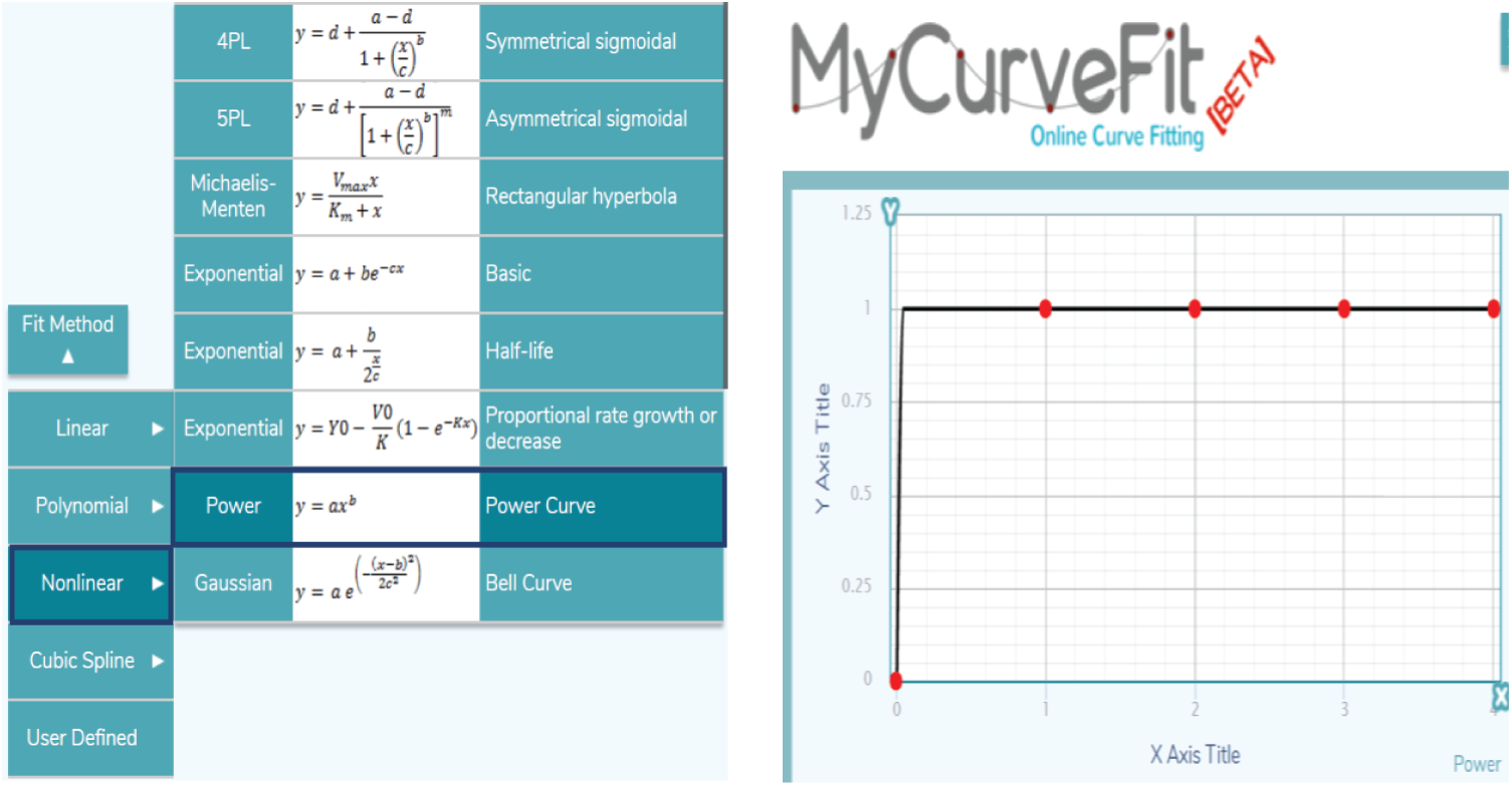
Figure 1: Curve fitting for the power equation

Then, the following covered demand constraints can be obtained:

yi-(∑j∈Nixj)[2.513459*10(-8)]=0∀i∈I(2)

When (∑j∈Nixj)=0, then yj = 0; this means no patients from the governorate i will be transported to the hospitals. However, when (∑j∈Nixj)>0 with values of 1, 2, 3 or 4, some patients are transported to the located hospitals. The range (1:4) is chosen since the number of governorates at a distance not exceeding Dc is limited by 4.

iii) Binary Constraints: All decision variables are binary (see Eqs. (3) and (4)).

yi∈{0,1}∀i∈I (3)

xj∈{0,1}∀j∈J (4)

Constraint (1) ensures that the total number of available field hospitals is not exceeded. The set of constraints (2) states that a governorate is not covered unless at least one established field hospital covers the patients in this governorate. Finally, constraints (3) and (4) are standard binary conditions.

iv) The Objective Function:

In this location problem, the objective is to maximize the number of patients covered by the established field hospitals (see Eq. (5)).

Maximize Z=∑i∈Iniyi(5)

5  A Real Application

A real application of the model is presented here. The model is applied to the 8 governorates in Upper Egypt, namely, Al-Fayoum, Beni Suef, El-Minya, Assiut, Sohag, Qena, Luxor, and Aswan. In view of the increase in cases of COVID-19 infections, it is necessary to increase the capacity of healthcare facilities by establishing additional field hospitals for medical quarantine and treating. This is to be done under limited finances, medical staff, and necessary equipment. The 8 governorates are briefly described below.

—Al-Fayoum:

Al-Fayoum governorate is located in Upper Egypt in a low location of the Western Desert, southwest of Cairo; it has an area of about 1,827 km2 and a population of 3.9 million people [23].

—Beni Suef:

Beni Suef governorate is located on the western bank of the River Nile, 110 km south of Cairo, and has a population of about 3.4 million people [24].

—El-Minya:

El-Minya governorate is located in the center of Egypt, on the River Nile. Its population is about 5.9 million [25].

—Assiut:

Assiut governorate is located in the center of Egypt on the River Nile. This governorate’s population is about 4.8 million people [26].

—Sohag:

Sohag governorate is located in Upper Egypt, south of the Assiut governorate and north of the Qena governorate. Its area is nearly 1547 km2, and it has a population of about 5.4 million people [27].

—Qena:

Qena governorate is located in Upper Egypt, 5–6 km from the River Nile and between the Arab and Libyan deserts. The area of the Qena governorate is about 1.851 km2, and it is home to about 3.5 million people [28].

—Luxor:

The city of Luxor was built on the ruins of the ancient capital city of Taibeh, Luxor governorate is located in Upper Egypt, its area is about 55 km2, and its population is about 1.4 million people [29].

—Aswan:

Aswan governorate has an area of about 679 km2 and is located directly on the eastern bank of the Nile River under the first waterfall; its population is about 1.6 million people [30].

Fig. 2 presents the geographic locations of the 8 governorates in Upper Egypt.

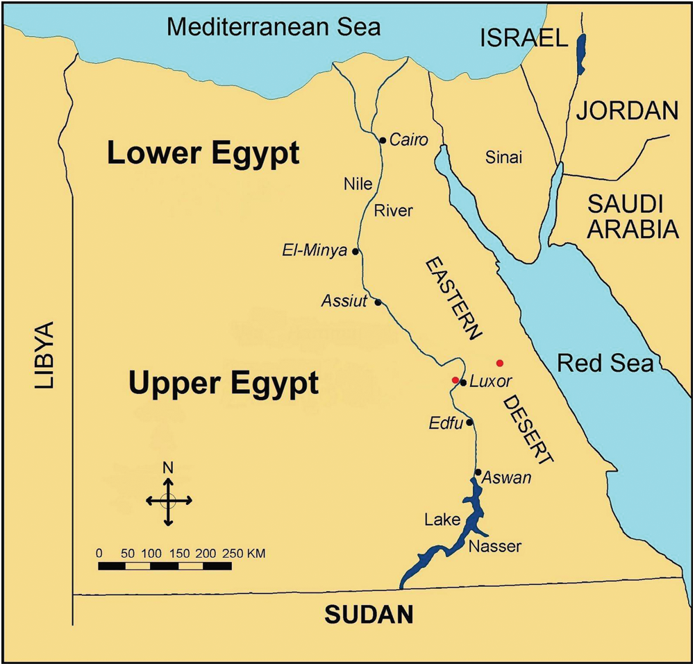
Figure 2: Upper Egypt governorates

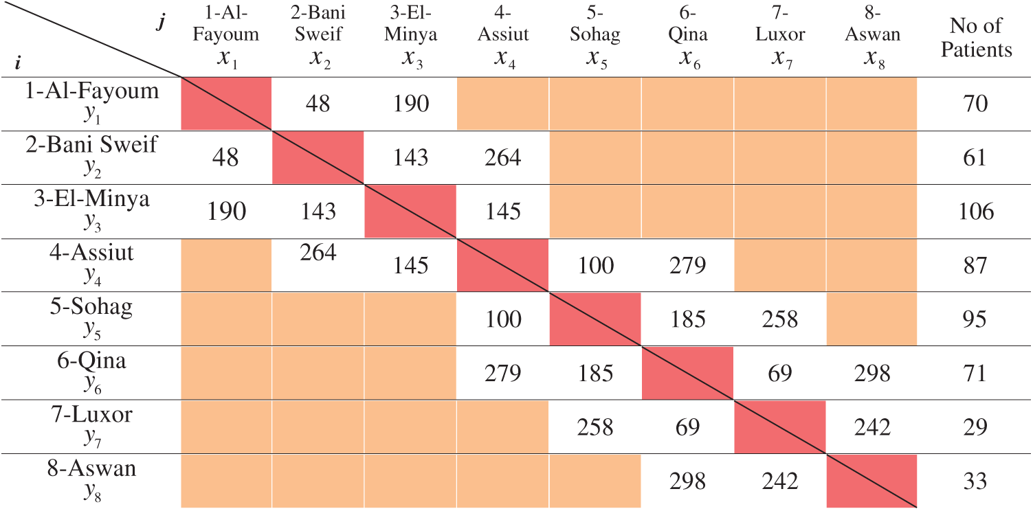
According to reference [31], di,j is the distance in km between a governorate i and a neighbor hospital j. Tab. 1 presents the candidate locations of the proposed field hospitals xj in the capital of each governorate, the distance di,j for the neighbor governorates to each field hospital that can be accommodated by that hospital, and the designation of decision variables (as in the mathematical model described in Section 3).

Table 1: Field hospitals, neighbor Governorates and related decision variables

The complete mathematical model for the application case study is formulated according to mathematical expressions (1–5). The proposed solution methodology is presented in the following section.

6  Proposed Solution Methodology

Metaheuristic approaches have been developed for complex optimization problems with continuous variables [32–41]. Reference [42] recently proposed a novel gaining–sharing knowledge-based optimization algorithm (GSK), setup on acquiring knowledge and share it with others throughout their lifetime. The original GSK solves optimization problems over continuous space, but it cannot solve a problem over binary space. Therefore, a new variant of GSK is introduced to solve the proposed mathematical model. A novel discrete binary gaining–sharing knowledge-based optimization algorithm (DBGSK) is proposed over discrete binary space with new binary junior and senior gaining and sharing stages.

There are many constraint handling techniques in the literature [43,44]. For example, reference [44] uses the augmented Lagrangian method, in which an unconstrained optimization problem was obtained from a constrained optimization problem. The proposed methodology is described in the below subsections.

6.1 Gaining–Sharing Knowledge-Based Optimization Algorithm (GSK)

An optimization problem with constraints is worked out as follows:

Minf(X);X=[x1,x2,…,xDim]s.to.gi(X)≤0;i=1,2,…,mX∈[αp,βp];p=1,2,…,Dim.

Here, f denotes the objective function; X=[x1,x2,…,xDim] are the decision variables; gi(X) are the inequality constraints; αp and βp are the lower and upper bounds of decision variables, respectively; and Dim represents the dimension of individuals. If the objective function is in maximization form, then minimization=-maximization.

The GSK algorithm contains two stages: Junior and senior gaining and sharing stages. All people acquire knowledge and share their views with others. People in the early stages of life (junior stage) gain knowledge from their networks, such as family members, relatives, and neighbors, and want to share this knowledge with others who might not be in their networks (this stems from a curiosity to explore others). These may not have the experience to categorize the people. In the same way, people in middle or later stages of life (senior stage) enhance their knowledge by interacting with various circles, such as friends, colleagues, and social media friends, and share their knowledge with the most suitable person (this stems from a desire to teach others). These people have the experience to judge other people and can categorize them as good or bad. The process described above can be mathematically formulated through the following steps.

Step 1:

To get a starting point of the optimization problem, the initial population must be obtained. The initial population is created randomly within the boundary constraints (Eq. (6)).

xtp0=αp+randp(βp-αp)(6)

Here, t is the number of populations; and randp denotes a random number uniformly distributed in the range 0–1.

Step 2:

The dimensions of junior and senior stages should be computed through Eqs. (7) and (8).

DimJ=Dim×(Genmax-GGenmax)k (7)

DimS=Dim-DimJ (8)

Here, k(> 0) denotes the learning rate. DimJ and DimS represent the dimensions for the junior and senior stages, respectively. Genmax is the maximum number of generations, and G is the generation.

Step 3:

Junior gaining–sharing knowledge stage: In this stage, the young people gain knowledge from their small networks and share their views with other people who may or may not belong to their network.

Thus, individuals are updated as follows.

     i)  According to the objective function values, individuals are arranged in ascending order. For every xt(t=1,2,…,NP), select the nearest best (xt −1) and worst (xt+1) to gain knowledge, and also choose randomly (xr) to share knowledge. The pseudo-code to update the individuals is presented in Fig. 3.

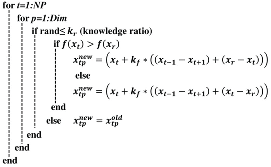
Figure 3: Pseudo-code for Junior gaining sharing knowledge stage

kf(> 0) is the knowledge factor.

Step 4:

Senior gaining–sharing knowledge stage: This stage comprises the impact and effect of other people (good or bad) on the individual. The updated individual can be determined as follows.

     i)  The individuals are classified into three categories (best, middle, and worst) after sorting individuals into ascending order (based on the objective function values).

The best individual=100p%(xbest), middle individual=Dim-2*100p%(xmiddle), and worst individual=100p%(xworst).

For every individual xt, choose the top and bottom 100p% individuals for gaining part and the middle individual for the sharing part. Therefore, the new individual is updated through the pseudo-code dictated in Fig. 4, where p∈[0,1] is the percentage of best and worst classes.

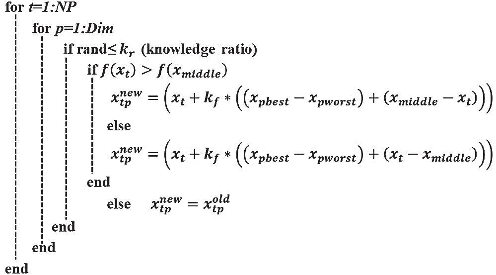
Figure 4: Pseudo-code of senior gaining sharing knowledge stage

6.2 Discrete Binary Gaining–Sharing Knowledge-Based Optimization Algorithm

To solve problems in discrete binary space, a novel discrete binary gaining–sharing knowledge-based optimization technique (DBGSK) is presented. In DBGSK, the new initialization and the working mechanism of both stages (junior and senior gaining–sharing stages) are introduced over discrete binary space, and the remaining algorithms remain the same. The working mechanism of DBGSK is described below.

Discrete Binary Initialization:

A first population is obtained in GSK using Eq. (8) and must be updated using Eq. (9) for the binary population.

xtp0=round(rand(0,1))(9)

The round operator is used to convert the decimal number into the nearest binary number.

Discrete Binary Junior Gaining and Sharing stage:

This stage is based on the original GSK with kf = 1. The individuals are updated in the original GSK using the pseudo-code presented in Fig. 6. This code contains two cases, which are defined for the discrete binary stage as below.

Case 1. When f(xr)<f(xt):

There are three different vectors (xt −1, xt+1, xr) that can take only two values (0 and 1). Therefore, a total of 23 combinations are possible (see Tab. 3). Furthermore, these eight combinations can be categorized into two different subcases [(a) and (b)], and each subcase has four combinations. The results of each possible combination are presented in Tab. 2.

Table 2: Results of the discrete binary junior gaining and sharing stage of case 1, kf=1

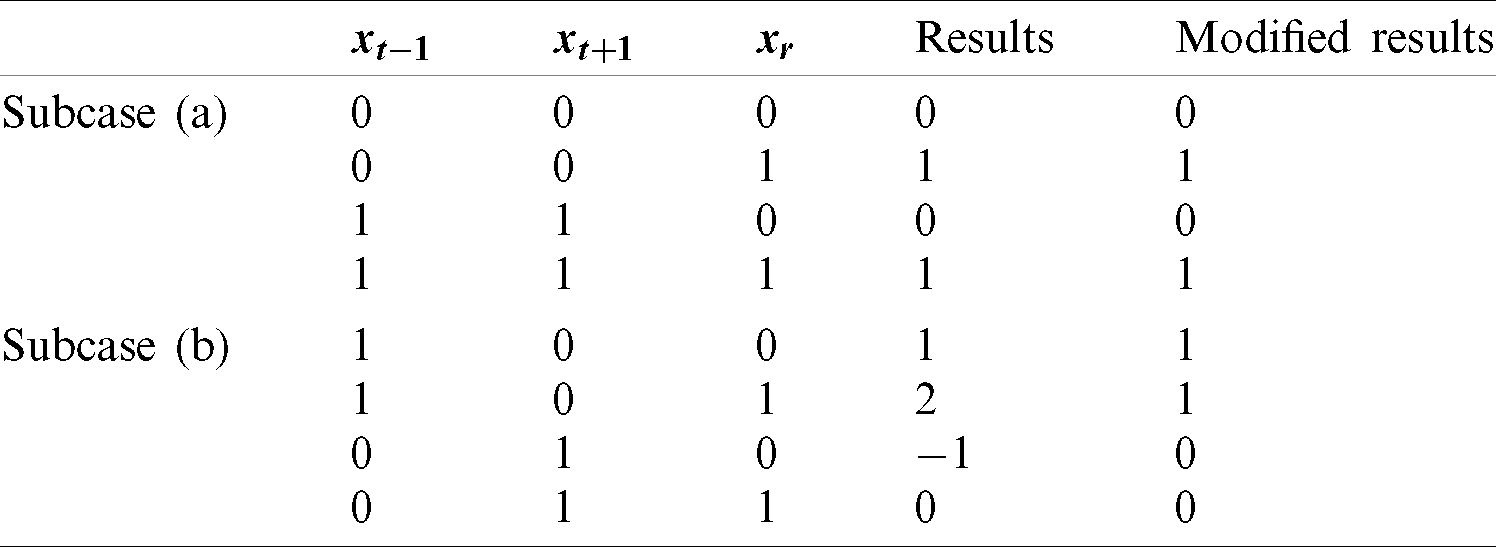
Subcase (a): If xt −1 is equal to xt+1, the result is equal to xr.

Subcase (b): When xt −1 is not equal to xt+1, then the result is the same as xt −1 by taking −1 as 0 and 2 as 1.

The mathematical formulation of Case 1 is as follows:

xtpnew={xr;ifxt-1=xt+1xt-1;ifxt-1≠xt+1.

Case 2. When f(xr)≥f(xt):

There are four different vectors (xt −1, xt, xt+1, xr) that consider only two values (0 and 1). Thus, there are 24 possible combinations (see Tab. 3).

Table 3: Results of the discrete binary junior gaining and sharing stage of case 2, kf=1

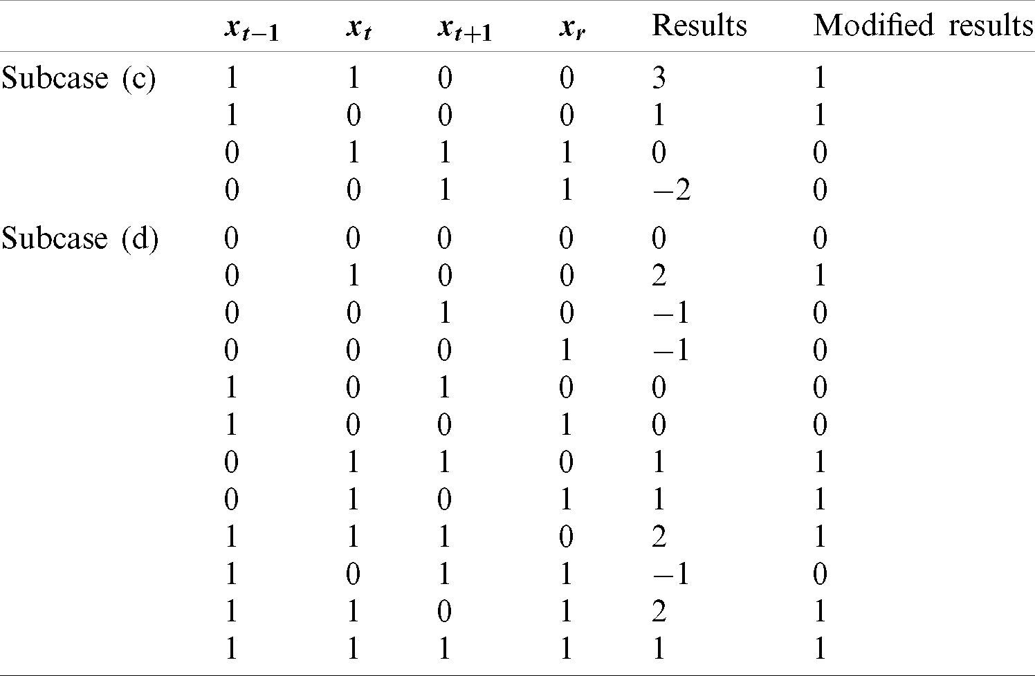
These 16 combinations can be divided into two subcases [(c) and (d)]; subcases (c) and (d) have 4 and 12 combinations, respectively.

Subcase (c): If xt −1 is not equal to xt+1, but xt+1 is equal to xr, the result is equal to xt −1.

Subcase (d): If any of the condition arises where xt-1=xt+1≠xr or xt-1≠xt+1≠xr or xt −1 = xt+1 = xr, the result is equal to xt by considering −1 and −2 as 0, and 2 and 3 as 1.

The mathematical formulation of Case 2 is

xtpnew={xt-1;ifxt-1≠xt+1=xrxt;Otherwise.

Discrete Binary Senior gaining and sharing stage:

The working mechanism of the discrete binary senior gaining and sharing stage is the same as the binary junior gaining and sharing stage with kf = 1. The individuals are updated in the original senior gaining–sharing stage using the pseudo-code presented in Fig. 7; this code also contains two cases. The two cases are further modified for the binary senior gaining–sharing stage, as described below.

Case 1. f(xmiddle)<f(xt):

Three different vectors (xbest,xmiddle,xworst) can assume only binary values (0 and 1), and thus a total of eight combinations are possible to update the individuals. These eight combinations can be classified into two subcases [(a) and (b)], each containing four different combinations. The combinations of this case are presented in Tab. 4.

Table 4: Results of discrete binary senior gaining and sharing stage of case 1 with kf=1

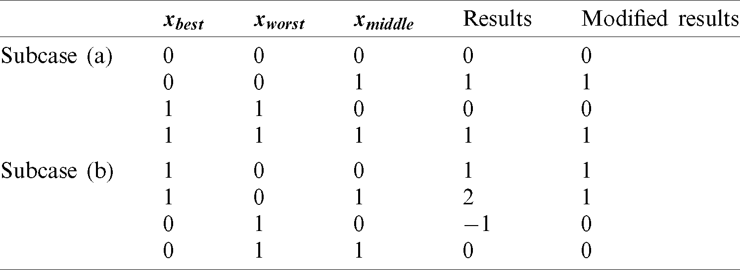
Subcase (a): If xbest is equal to xworst, then the obtained results are equal to xmiddle.

Subcase (b): If xbest is not equal to xworst, then the results are equal to xbest while assuming −1 or 2 according to the nearest binary value (0 or 1, respectively).

Case 1 can be mathematically formulated in the following way:

xtpnew={xmiddle;ifxbest=xworstxbest;ifxbest≠xworst.

Case 2. f(xmiddle)>f(xt):

There are four different binary vectors (xbest,xmiddle,xworst,xt), yielding a total of 16 combinations. The 16 combinations are also divided into two subcases (c) and (d). The subcases (c) and (d) contain 4 and 12 combinations, respectively. The subcases are explained in detail in Tab. 5.

Table 5: Results of discrete binary senior gaining and sharing stage of case 2 with kf=1

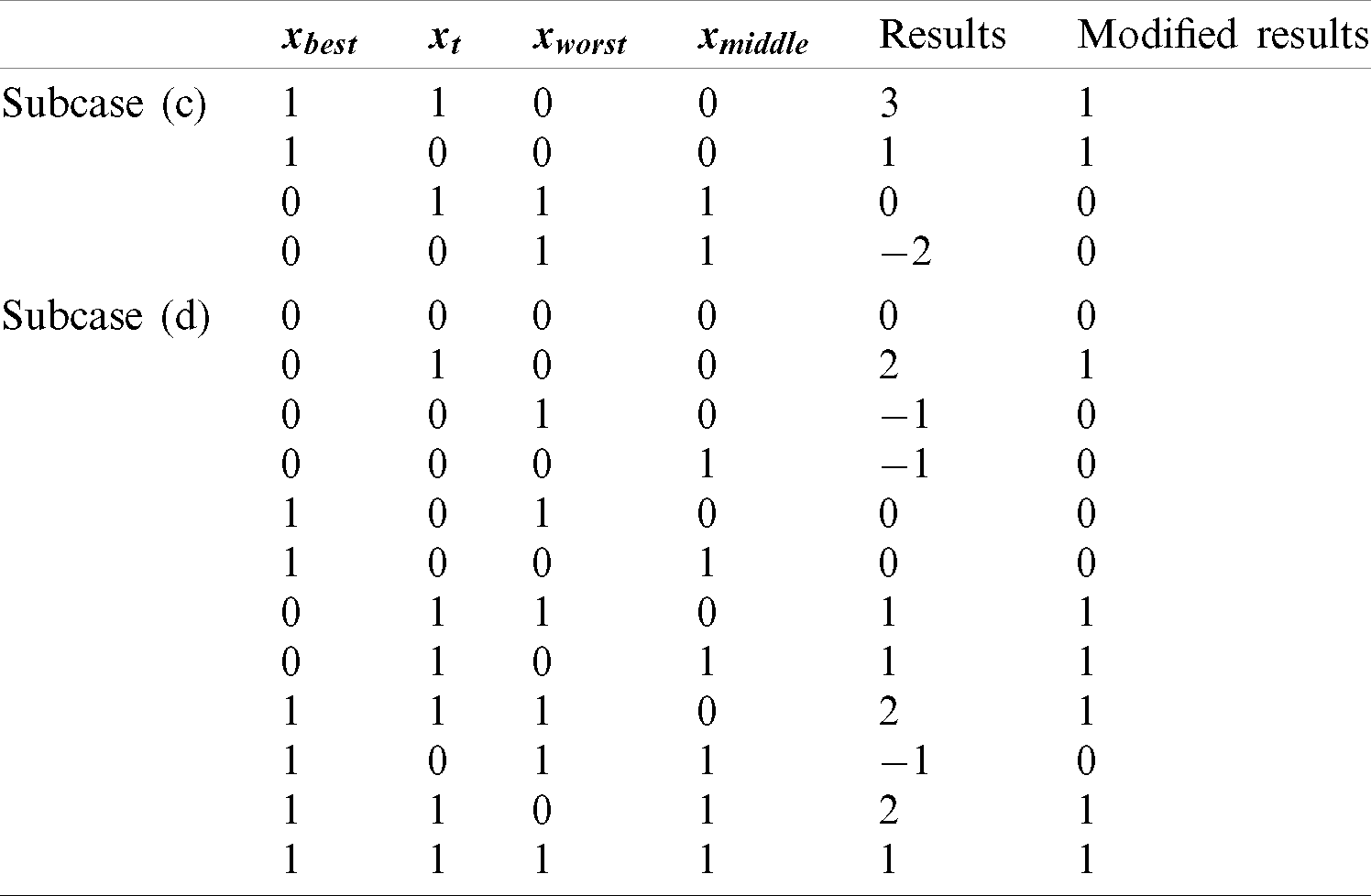
Subcase (c): When xbest is not equal to xworst and xworst is equal to xmiddle, then the obtained results are equal to xbest.

Subcase (d): If any case arises other than (c), then the obtained result is equal to xt by taking −2 and −1 as 0 and 2 and 3 as 1.

The mathematical formulation of Case 2 is

xtpnew={xbest;ifxbest≠xworst=xmiddlext;Otherwise.

The pseudo-code of DBGSK is presented in Fig. 5.

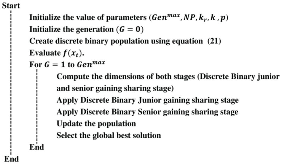
Figure 5: Pseudo-code for DBGSK

7  Experimental Results

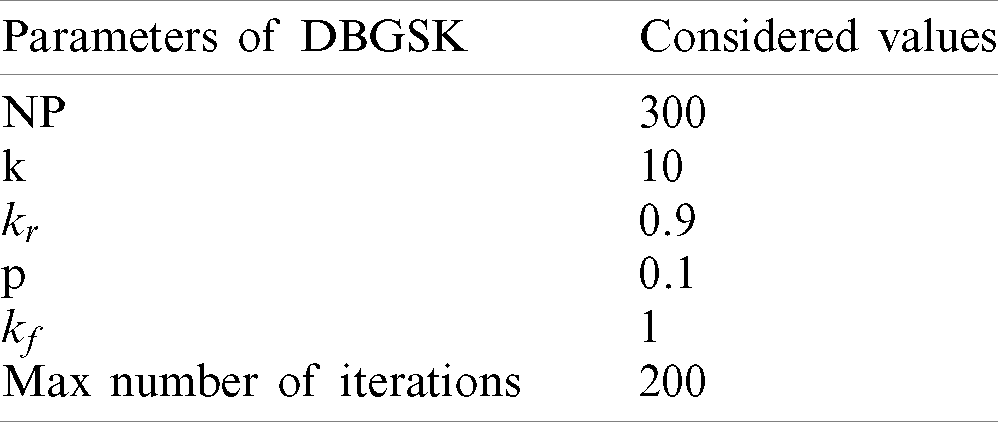
The proposed mathematical model employs the proposed novel DBGSK algorithm, the parameters of which are presented in Tab. 6.

Table 6: Numerical Values of parameters

DBGSK runs on an Intel ® CoreTM i5-7200U CPU@2.50 GHz and 4 GB RAM, and is coded in MATLAB R2015a. To get the compromise or the effective solution, 30 independent runs are completed. The results obtained by DBGSK are presented in Tab. 7, including the best, median, average, worst solutions, and standard deviations.

Table 7: Statistical results using DBGSK

It can be obviously seen in Tab. 7 that the DBGSK algorithm reaches the optimal solution consistently over the 30 runs with zero standard deviation, which proves its outstanding robustness. Moreover, Fig. 6 shows the convergence graph of the solutions of the proposed mathematical model using 3 field hospitals. After the 14th iteration, the model converges to the global optimal solution (552), which shows the high convergence speed of DBGSK.

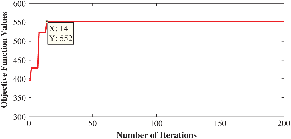
Figure 6: Convergence graph of DBGSK

The optimum solutions for the problem with different numbers of field hospitals to be established (1, 2, or 3) are presented in Fig. 7. We notice that the covered governorates in the case of establishing one field hospital in Assiut are Beni Suef, El-Minya, Sohag, and Qina, and the total number of patients = 333. When establishing 2 field hospitals, they are to be built in Beni Suef and Assiut, or in El-Minya and Assiut; in this case, the covered governorates are Al-Fayoum, Beni Suef, El-Minya, Assiut, Sohag, and Qina, and the total number of patients=490. In the case of establishing 3 field hospitals, they are to be built in Beni-Suef), Assiut, and Qina or in El-Minya, Assiut, and Qina; in this case, all 8 governorates are covered, and the total number of patients=552. The decision-maker can choose the best solution from these three solutions according to the available resources (medical staff, accommodation, devices, and materials).

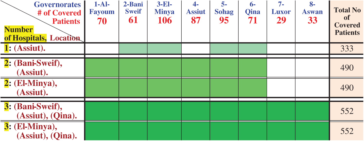
Figure 7: Covered patients for different numbers of the established field hospitals

8  Conclusions and Directions for Future Research

The main contributions of this paper can be summarized as follows.

     i)  A variant of the maximal coverage location model to formulate establishing of field hospitals for COVID-19 problem is proposed. The model is designed to suit a special problem formulation for placing some field hospitals in candidate locations while maximizing the number of covered patients.

    ii)  A nonlinear binary constrained model is formulated for the given problem. The binary decision variables are establishing field hospitals in the chosen candidate sites and covering patients in different governorates.

   iii)  The designed mathematical model and method for obtaining the optimum solution are applied to 8 governorates in Upper Egypt with different numbers of hospitals to be established.

    iv)  The problem is solved by a novel discrete binary gaining–sharing knowledge-based optimization algorithm (DBGSK), which involves two main stages: Discrete binary junior and senior gaining and sharing stages, with a knowledge factor kf = 1. DBGSK is a discrete binary variant of GSK that solves the problem with binary decision variables.

     v)  DBGSK can find the solutions of the problem, with good robustness and convergence.

Suggestions for future research are as follows.

     i)  To propose other mathematical models’ formulations for the same problem comprising designing the objective function(s), decision variables, and constraints, and then to compare various proposed mathematical models.

    ii)  To continue applying the problem to other regions of the country, to the whole country, and to other countries.

   iii)  To build an online decision support system that can handle repetitive situations with timely updated data and, in turn, update the locations of field hospitals for COVID-19 to reflect the updated data.

    iv)  To check the performance of the DBGSK approach in solving different complex optimization problems, and with different kinds of constraint handling methods.

Acknowledgement: The authors are grateful to the Deanship of Scientific Research, King Saud University, KSA, for funding through the Vice Deanship of Scientific Research Chairs.

Funding Statement: This research was funded by Deanship of Scientific Research, King Saud University, through the Vice Deanship of Scientific Research.

Conflicts of Interest: The authors declare that they have no conflicts of interest to report regarding the present study.

This work is licensed under a Creative Commons Attribution 4.0 International License, which permits unrestricted use, distribution, and reproduction in any medium, provided the original work is properly cited.