Computers, Materials & Continua DOI:10.32604/cmc.2021.015115
Article

A New BEM for Fractional Nonlinear Generalized Porothermoelastic Wave Propagation Problems

Mohamed Abdelsabour Fahmy1,2,*

1Department of Mathematics, Jamoum University College, Umm Al-Qura University, Alshohdaa, 25371, Jamoum, Saudi Arabia
2Department of Basic Sciences, Faculty of Computers and Informatics, Suez Canal University, New Campus, Ismailia, 41522, Egypt
*Corresponding Author: Mohamed Abdelsabour Fahmy. Email: maselim@uqu.edu.sal
Received: 06 November 2020; Accepted: 24 January 2021

Abstract: The main purpose of the current article is to develop a novel boundary element model for solving fractional-order nonlinear generalized porothermoelastic wave propagation problems in the context of temperature-dependent functionally graded anisotropic (FGA) structures. The system of governing equations of the considered problem is extremely very difficult or impossible to solve analytically due to nonlinearity, fractional order diffusion and strongly anisotropic mechanical and physical properties of considered porous structures. Therefore, an efficient boundary element method (BEM) has been proposed to overcome this difficulty, where, the nonlinear terms were treated using the Kirchhoff transformation and the domain integrals were treated using the Cartesian transformation method (CTM). The generalized modified shift-splitting (GMSS) iteration method was used to solve the linear systems resulting from BEM, also, GMSS reduces the iterations number and CPU execution time of computations. The numerical findings show the effects of fractional order parameter, anisotropy and functionally graded material on the nonlinear porothermoelastic stress waves. The numerical outcomes are in very good agreement with those from existing literature and demonstrate the validity and reliability of the proposed methodology.

Keywords: Boundary element method; fractional-order; nonlinear generalized porothermoelasticity; wave propagation; functionally graded anisotropic structures; Cartesian transformation method

1  Introduction

The fractional order calculus (FOC) is the branch of mathematical analysis dealing with non-integer order calculus and its applications. The essential viewpoints are sketched out for fractional calculus theory in [1] and for fractional calculus applications in [2–6]. FOC is nowadays extremely popular due to its applications in different fields such as diffusion equation, quantum mechanics, nanotechnology, solid mechanics, continuum mechanics, biochemistry, wave propagation theory, polymers, robotics and control theory, finance and control theory, electrochemistry, electrical engineering, fluid dynamics, signal and image processing, biophysics, electric circuits, viscoelasticity, electronics, field theory, group theory, etc.

Several researchers have contributed to the background of fractional calculus [7–9]. Recently, Yu et al. [10] introduced new definitions of fractional derivative in the context of thermoelasticity. Research on generalized thermo-elasticity theories [11] has attracted much attention from many scientists, among which are research in magneto-thermoelasticity [12], visco-thermoelasticity [13,14] and micropolar-thermoelasticity [15,16].

Because of computational complexity in solving complex fractional thermoelasticity problems not having any general analytical solution, computational techniques should be used to solve such problems. Among these computational techniques are the boundary element method (BEM) that has been used for magneto thermoviscoelasticity [17,18], computerized engineering models [19,20], and design sensitivity and optimization [21,22] and nonlinear problems [23–26]. The BEM presents an attractive alternative numerical method to the domain methods for the investigation of thermoelastic wave propagation problems, like finite element method (FEM) [27–29] and finite volume method (FVM) [30–32]. The main feature of BEM over the domain type methods is that it requires boundary-only discretization of the domain under consideration. This feature has significant importance for solving complex thermoelastic problems with fewer elements, and requires very little computational cost, much less preparation of input data, and therefore easier to use.

In the present paper, we introduce a new boundary element model for solving fractional-order nonlinear generalized porothermoelastic wave propagation problems. The nonlinear terms are treated using the Kirchhoff transformation. The domain integrals were treated using the Cartesian transformation method. In the proposed BEM technique, the temperature and displacement distributions were calculated using a partitioned semi-implicit predictor–corrector coupling algorithm. Then, we can obtain the propagation of porothermoelastic stress waves in temperature-dependent FGA structures. Numerical results demonstrate the validity, accuracy and efficiency of our proposed model and technique.

2  Formulation of the Problem

The geometry of the considered problem is depicted in Fig. 1. The governing equations for fractional-order nonlinear generalized porothermoelastic wave propagation problems in the context of FGA structures can be written as [33]

σij,j+ρFi=ρu¨i+ϕρFv¨i(1)

where σij is the mechanical stress tensor, ρ is the bulk density, ρF is the fluid density, Fi is the bulk body forces, ϕ is the porosity, ui is the solid displacement and vi is the fluid–solid displacement.

ζ̇+qi,i=ℂ¯i(2)

where ζ is the variation of the fluid volume per unit reference volume, q is the instantaneous flux and ℂ¯i is the source term.

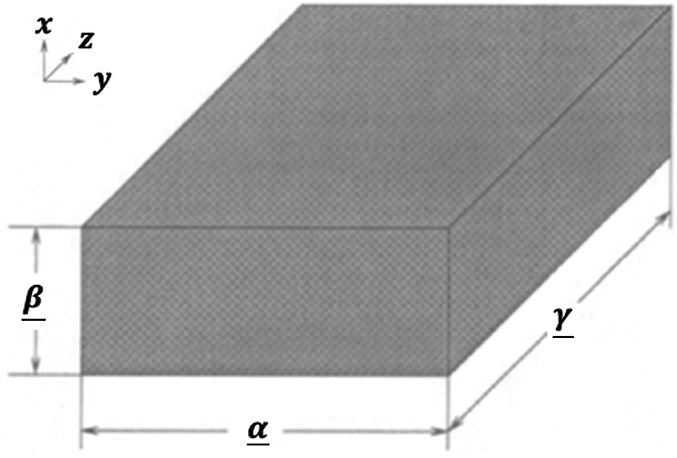
Figure 1: Geometry of the considered problem

The fractional nonlinear heat conduction equation can be expressed in non-dimensionless form as

DτaT(x,t)=ξ∇[λ(T)∇T(x,t)]+ξh(x,T,t),ξ=1ρ(T)c(T)(3)

in which

σij=(x+1)m[Cijkleδij-Aδijp-βij(T+τ1Ṫ)] (4)

qi=-k¯(x+1)m(p,i+ρFu¨i+ρ0+ϕρFϕv¨i),ζ=[Auk,k+ϕ2Rp] (5)

where εij=12(ui,j+uj,i), e=εii and A=ϕ(1+QR).

in which the heat source function h(X,T,t) can be written as

h(x,T,t)=h¯(x,T,t)-δ2nλṪ,ij+βijT0[Åδ1nu̇i,j+(τ0+δ2n)u¨i,j]+ρcα[(τ0+δ1nτ2+δ2n)T¨](6)

where T is the temperature,λ is the thermal conductivity, Cijkl is the constant elastic moduli, A is the Biot’s effective stress coefficient, p is the fluid pressure, βij is the stress-temperature coefficients, k¯ is the permeability, T0 is the reference temperature, Å is a unified parameter that introduces all generalized thermoelasticity theories into a unified system of equations, Q and R are solid–fluid coupling parameters, τ0, τ1, and τ2 are relaxation times, ρ0=ηϕρF and η is the shape factor.

According to finite difference scheme of Caputo at times (f+1)Δτ and fΔτ, we obtain [34]

DτaTf+1+DτaTf≈∑J=0kWa,J(Tf+1-J(x)-Tf-J(x))(7)

where

Wa,0=(Δτ)-aΓ(2-a)andWa,J=Wa,0((J+1)1-a-(J-1)1-a)(8)

On the basis of Eq. (7), the fractional heat conduction Eq. (3) can be expressed as

Wa,0Tf+1(x)-λ(x,T)T,iif+1(x)-λ,i(x,T)T,if+1(x)=Wa,0Tf(x)-λ(x)T,iif(x)-λ,i(x,T)T,jf(x)-∑J=1fWa,J(Tf+1-J(x)-Tf-J(x))+hmf+1(x,T,τ)+hmf(x,T,τ)(9)

where J=1,2,…,F and f=0,1,2,…,F.

3  BEM Implementation for Temperature Field

By using the transformation of Kirchhoff Θ=∫T0Tλ(T¯)λ0dT¯, Eq. (3) can be written as [35]

∇2Θ(x,t)+1λ0h(x,Θ,t)=ρ(Θ)c(Θ)λ(Θ)∂Θ(x,t)∂t(10)

The decomposition of the right-hand side of (10) into linear and nonlinear sections, yields

∇2Θ(x,t)+1λ0h(x,Θ,t)=ρ0c0λ0∂Θ(x,t)∂t+Nl(x,Θ,Θ̇)(11)

The nonlinear section can be written as

Nl(x,Θ,Θ̇)=[ρ(Θ)c(Θ)λ(Θ)-ρ0c0λ0]Θ̇(12)

Based on [24], we can write (11) into the following form

∇2Θ(x,t)+1λ0hNl(x,Θ,Θ̇,t)=ρ0c0λ0∂Θ(x,t)∂t(13)

where

hNl(x,Θ,Θ̇,t)=h(x,Θ,t)+[ρ0c0-λ0λ(Θ)ρ(Θ)c(Θ)]Θ̇(14)

Now, by using the fundamental solution of (9), we can write the boundary integral equation corresponding to (13) as [36]

C(P)Θ(P,tn+1)+a0∫Γ∫tntn+1Θ(Q,τ)q*(P,tn+1;Q,τ)dτdΓ=a0∫Γ∫tntn+1q(Q,τ)Θ*(P,tn+1;Q,τ)dτdΓ+a0λ0∫Ω∫tntn+1hNl(Q,Θ,Θ̇,τ)Θ*(P,tn+1;Q,τ)dτdΩ+∫ΩΘ(Q,tn)Θ*(P,tn+1;Q,tn)dΩ,a0=λ0ρ0c0(15)

By substituting of Θ(P,tn+1)=2Θ(P,tn+(1/2))-Θ(P,tn) in (15), we get

2C(P)Θ(P,tn+(1/2))-12π∫ΓΘ(Q,tn+(1/2))rexp[-r24a0Δt]∂r∂ndΓ=14π∫Γq(Q,tn+(1/2))Ei(r24a0Δt)dΓ+14πλ0∫ΩhNl(Q,Θn+(1/2),Θ̇n+(1/2),tn+(1/2))Ei(r24a0Δt)dΩ+14πa0Δt∫ΩΘ(Q,tn)exp(-r24a0Δt)dΩ+C(P)Θ(P,tn)(16)

where Θn+(1/2)=Θn+Θn+12, tn+(1/2)=tn+tn+12, and Θ̇n+(1/2)=Θn+1-ΘnΔt

Now, the domain integrals in Eq. (16) can be computed using CTM. Thus, the unknown boundary values can be calculated from the following system

HΘΓ=GQΓ+F+FNl(17)

where ΘΓ and QΓ are M′ dimension vectors, and H and G are M′×M′ dimension matrices.

Thus, the unknown internal values can be calculated from the following system

ΘΩ=G^QΓ-H^ΘΓ+F^+F^Nl(18)

If we have assumed that the time step size is constant, then, H, G, H^, and G^ can be computed at all time steps. Also, F, FNl, F^, and F^Nl can be computed at all time steps using CTM.

3.1 CTM Evaluation of the Domain Integrals with Irregularly Spaced Data Kernels

Now, we are considering the following regular domain integral [37,38]

I=∫Ωp(x1,x2)dΩ(19)

Based on Khosravifard et al. [39], we can write the domain integral (19) as follows

I=∫Γ(∫αx1p(x1′,x2)dx1′)dx2(20)

where

α=x1min+x1max2(21)

By applying the composite Gaussian quadrature method to (19), we obtain

I=∑k=1K∫Γk∫αx1p(x1′,x2)dx1′dx2(22)

which can be written as

I=∑k=1KJk∑i=1Nwi∑l=1LJl∑j=1Jwjp(x1(ηj),x2(ηi))(23)

By implementing the radial point interpolation method (RPIM) [40], we can write

p(x1,x2)=∑i=1Mϕi(x1,x2)pi=ΦTP(24)

where M equals the summation of boundary nodes M′ and internal points M′′.

Based on [40], the function p(x1,x2) may be described as

p(x)=∑i=1nαiψi(x)+∑j=1m¯bjuj(x)=ΨT(x)a+uT(x)b=[ΨT(x)uT(x)]{ab}(25)

To build the RPIM shape functions, we applied the following Gaussian radial basis function

ψi(x)=exp[-ac(Ridc)2](26)

where αi and bj are unknown coefficients which can be computed from the following system

∑i=1nαiψi(xi)+∑j=1m¯bjuj(xi)=p(xi),i=1,2,…,n(27)

and the following m¯ conditions

∑i=1nαiuj(xi)=0,j=1,2,…,m¯(28)

By using Eqs. (27) and (28), we can express αi and bj as

{ab}=BP(29)

Thus, based on [40], and using (29), we can write Eq. (25) in the following form

p(x)=[ ψT(x)uT(x) ]BP=ϕTP(30)

Thus, we have

I=∑k=1KJk∑i=1Nwi∑l=1LJl∑j=1Jwj∑r=1Mprϕr(x1(ηj),x2(ηi))(31)

which can be written as

I=∑q=1Mγqpq=γTp(32)

where p contains boundary and internal p values.

3.2 CTM Evaluation of the Domain Integrals with Regularized Kernels

We now consider the following domain integrals that appear in the integral Eq. (16)

I1=∫ΩhNI(Q,Θn+(1/2),Θ̇n+(1/2),tn+(1/2))Ei(r24a0Δt)dΩ (33)

I2=∫ΩΘ(Q,tn)exp[-r24a0Δt]dΩ (34)

where Ei(x)=-0.57721566+∑n=1∞(-1)n-1xnn.n!-ln(x)

According to [25], the weakly singular in (33) can be regularized to obtain

I1=γT(p1+p2)+I′(P)(35)

where

I′(P)=2hNI(P,Θn+(1/2),Θ̇n+(1/2),tn+(1/2))D1(P)(36)

and

D1(P)=∫Γ[ln(1r)dx1)]dx2=∫Γ[-r1lnr-r2tan-1(r1r2)+r1]dx2(37)

Also, the domain integral in (34) can be regularized to obtain

I2=γTp3+I″(P)(38)

where

I″(P)=Θ(P,tn)D2(P,Δt)(39)

and

D2(P,Δt)=∫Γ∫exp[-r24a0Δt]dx1dx2=πa0Δt∫Γexp(-r224a0Δt)erf(r12a0Δt)dx2,erf(a)=2π∫0αexp(-x2)dx(40)

Hence, from (18) we get

𝕒X=𝕓(41)

where 𝕒 is an unknown matrix, while X and 𝕓 are known matrices.

4  BEM Implementation for Displacement Field

Based on the weighted residual technique, we can write Eqs. (1) and (2) as follows

∫R(σij,j+Ui)ui*dR=0 (42)

∫R(qi,i+ζ̇i-ℂi)pi*dR=0 (43)

where

σij,j=(x+1)m[Cijkluk,lj-Aδijp,j-βij(T,j+τ1Ṫ,j)]++mx+1σijqi,i=-k¯(x+1)m(p,ii+ρFu¨i,i+ρ0+ϕρFϕv¨i,i)+mx+1qi

in which Ui=ρFi-ρu¨i-ϕρFv¨i, and ui* and pi* are weighting functions.

On using integration by parts for the first term of Eqs. (42) and (43), we get

-∫Rσijui,j*dR+∫RUiui*dR=-∫S2λiui*dS (44)

-∫Rqpi,j*dR+∫Rζ̇ipi*dR-∫Rℂipi*dR=-∫S4Lipi*dS (45)

Based on Fahmy [24], elastic stress can be expressed as

∫Rσij,j*uidR=-∫Sui*λidS-∫Spi*LidS+∫Sλi*uidS+∫SLi*pidS(46)

which can be expressed as

Cn𝕢n=-∫S𝕡*𝕢dS+∫S𝕢*𝕡dS+∫S𝕒*pdS+∫S𝕓*∂p∂ndS(47)

where

Cn=[C11C12C21C22],𝕢*=[u11*u12*ω13*u21*u22*ω23*u31**u32**ω33**],𝕡*=[λ11*λ12*μ13*λ21*λ22*μ23*λ31**λ32**μ33**]𝕢=[u1u2ω3],𝕡=[λ1λ2μ3],𝕒*=[a1*a2*0],𝕓*=[b1*b2*0]

Now, we consider the following definitions

𝕢=ψ𝕢j,𝕡=ψ𝕡j,p=ψ0pj,∂p∂n=ψ0(∂p∂n)j(48)

Substituting above definitions into (47), we get

Cn𝕢n=∑j=1Ne[-∫Γj𝕡*ψdΓ]𝕢j+∑j=1Ne[∫Γj𝕢*ψdΓ]𝕡j+∑j=1Ne[∫Γj𝕒*ψ0dΓ]pj+∑j=1Ne[∫Γj𝕓*ψ0dΓ](∂p∂n)j(49)

which after integration can be written as

Ci𝕢i=-∑j=1Ne𝔿^ij𝕢j+∑j=1Ne𝔾^ij𝕡j+∑j=1Ne𝕒^ijpj+∑j=1Ne𝕓^ij(∂p∂n)j(50)

where

𝔿ij={𝔿^ijifi≠j𝔿^ij+Ciifi=j(51)

Now, we can write (50) as

∑j=1Ne𝔿ij𝕢j=∑j=1Ne𝔾^ij𝕢j+∑j=1Ne𝕒^ijpj+∑j=1Ne𝕓^ij(∂p∂n)j(52)

which can be expressed as follows

𝔿𝕈=𝔾𝕇+𝕒𝕚+𝕓𝕛(53)

where the vectors 𝕈, 𝕇, 𝕚, and 𝕛 are displacements, tractions, pore pressure, and pore pressure gradients, respectively.

Substituting the boundary conditions into (54), we obtain the following system of equations

𝔸𝕏=𝔹(54)

in which 𝔸 represents unknown matrix, while 𝕏 and 𝔹 represent known matrices.

According to Breuer et al. [41], a robust and efficient partitioned semi-implicit predictor–corrector coupling algorithm was implemented with GMSS [42] for solving the resulting linear Eqs. (41) and (54) arising from the boundary element discretization, where poro-thermo-elastic coupling is considered instead of fluid-structure-interaction coupling.

5  Numerical Results and Discussion

The proposed BEM technique which is based on the coupling algorithm [41], should be applied to a wide variety of fractional-order nonlinear porothermoelastic wave propagation problems.

In the present paper, we considered the temperature-dependent properties of anisotropic porous copper material, where the specific heat and density are tabulated in Tab. 1 [43].

Table 1: Temperature-dependent specific heat and density of porous copper material

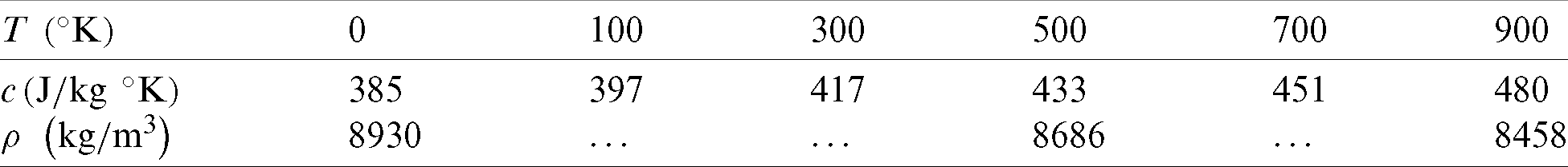
The thermal conductivity is given by

λ=400(1-T6000)

The domain boundary of the current problem has been discretized into 42 boundary elements and 68 internal points as depicted in Fig. 2.

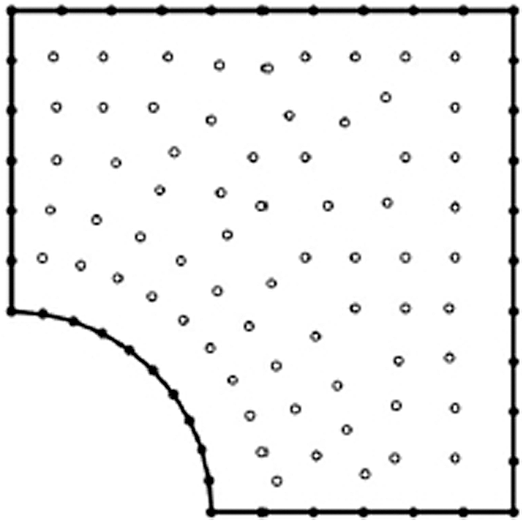
Figure 2: Boundary element model of the considered problem

Figs. 3–5 illustrate the propagation of nonlinear thermal stress waves σ11, σ12, and σ22 for different values (a=0.4,0.7 and 1.0) of the fractional order parameter (FOP). It can be seen from these figures that the FOP has a great influence on the nonlinear thermal stress waves of FGA porous structures.

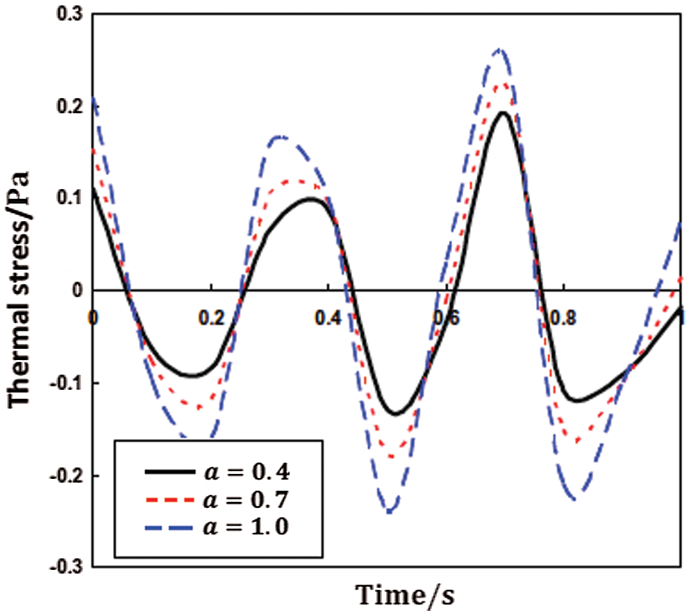
Figure 3: Propagation of the nonlinear thermal stress σ11 waves with time t for different values of the fractional-order parameter

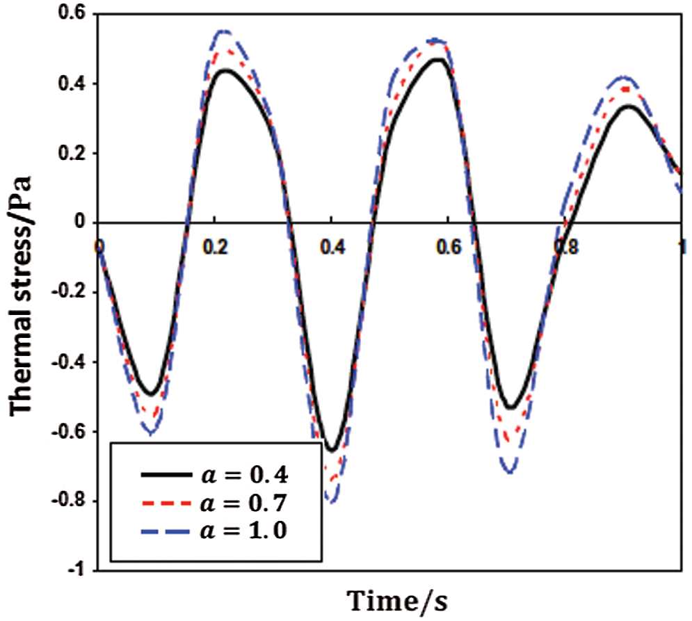
Figure 4: Propagation of the nonlinear thermal stress σ12 waves with time t for different values of the fractional-order parameter

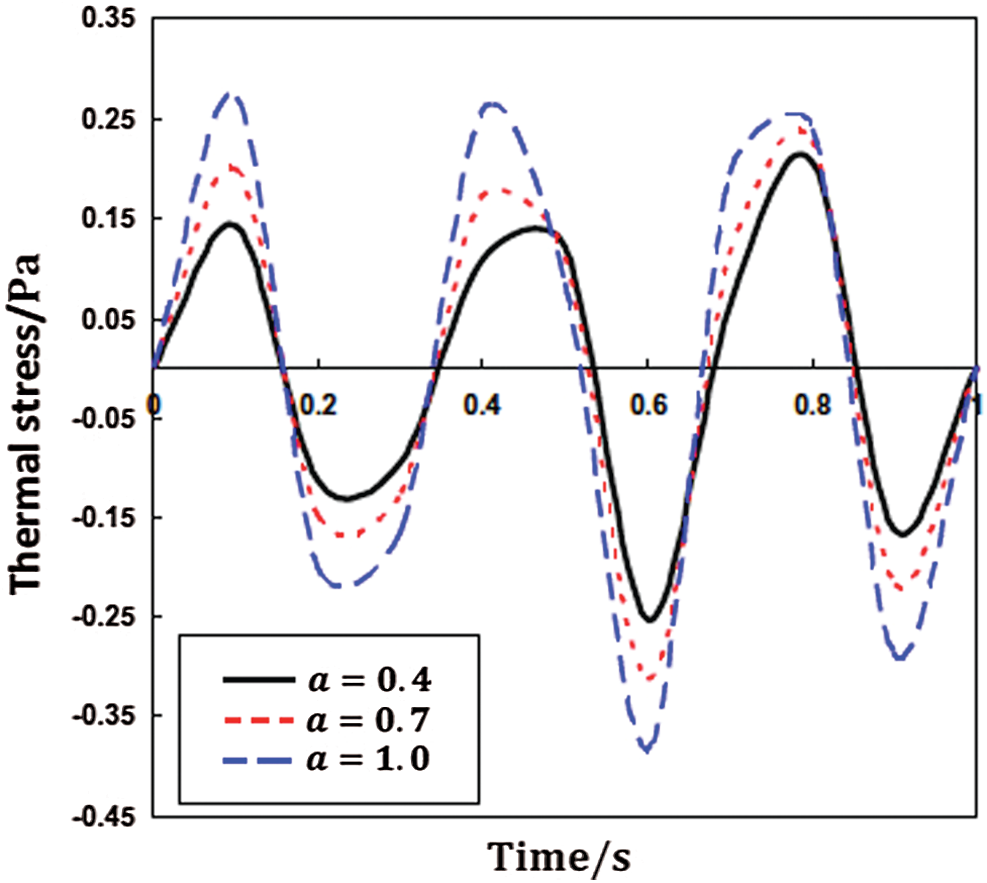
Figure 5: Propagation of the nonlinear thermal stress σ22 waves with time t for different values of the fractional-order parameter

According to the relationship of elastic constants for anisotropic, isotropic, and orthotropic materials [44]. We therefore considered these three materials in the current study.

Figs. 6–8 show the propagation of nonlinear thermal stress waves σ11, σ12, and σ22 for anisotropic, isotropic and orthotropic functionally graded porous structures. It can be shown from these figures that the effects of anisotropy are very pronounced.

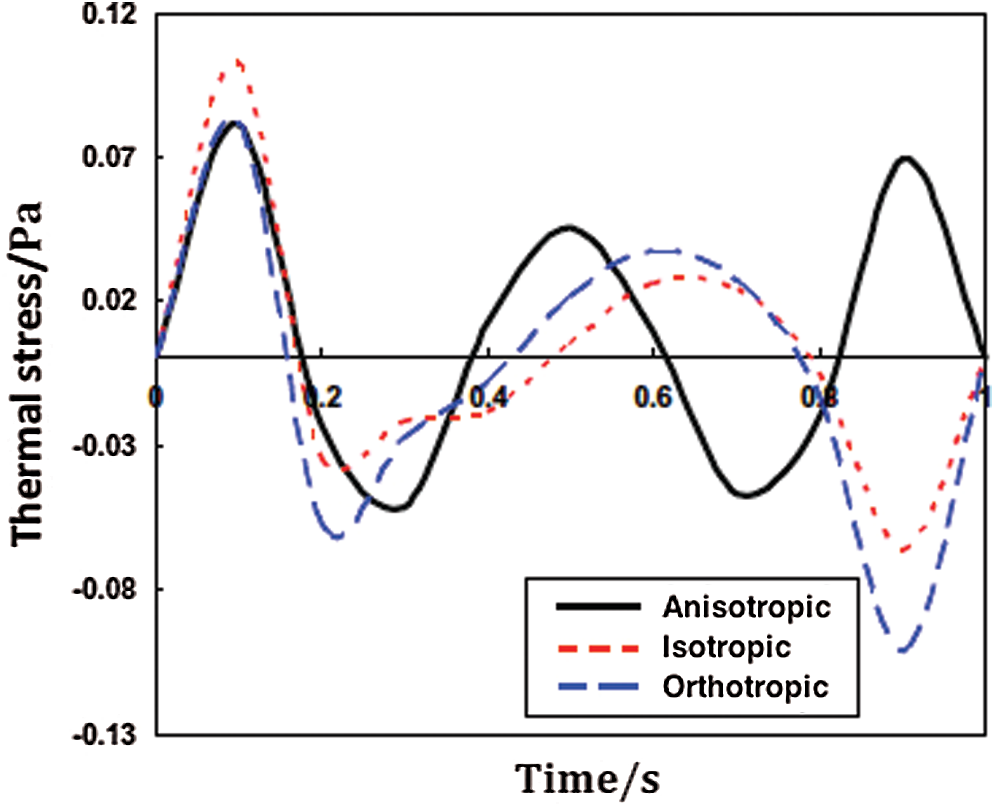
Figure 6: Propagation of the nonlinear thermal stress σ11 waves with time t for isotropic, orthotropic and anisotropic porous materials

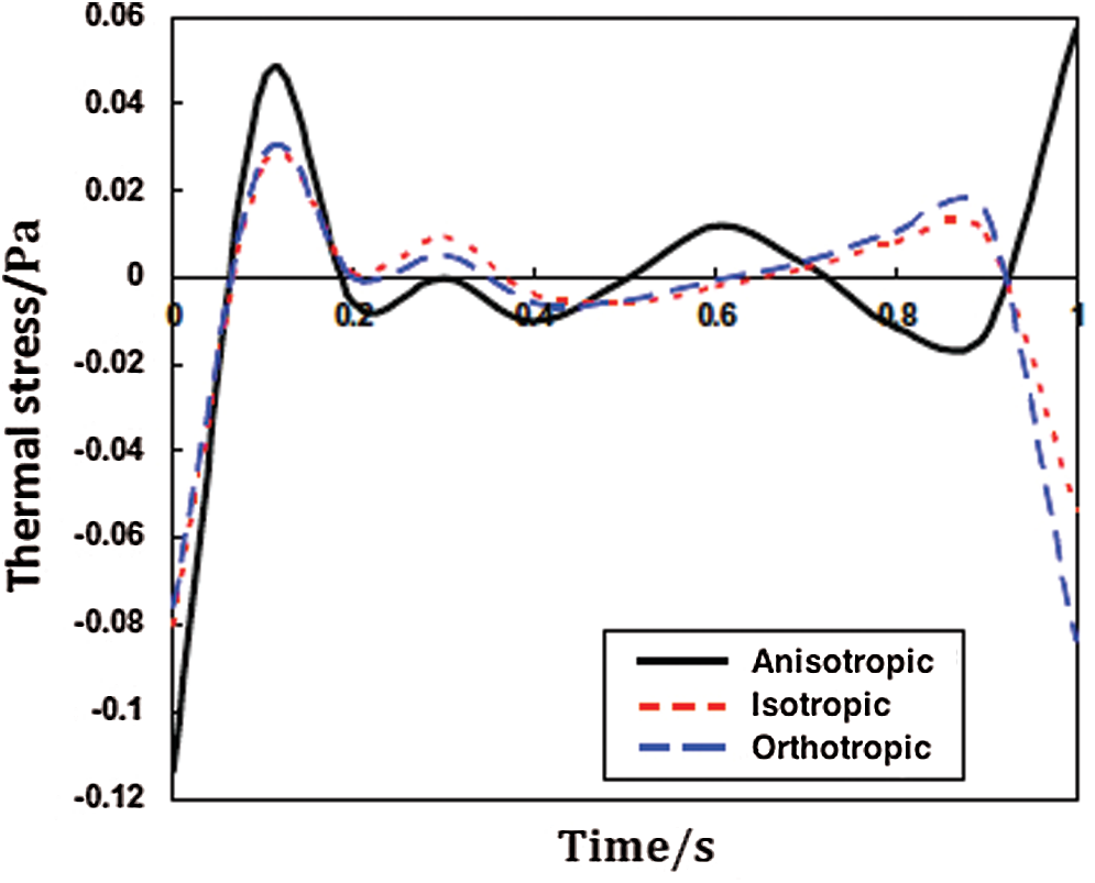
Figure 7: Propagation of the nonlinear thermal stress σ12 waves with time t for isotropic, orthotropic and anisotropic porous materials

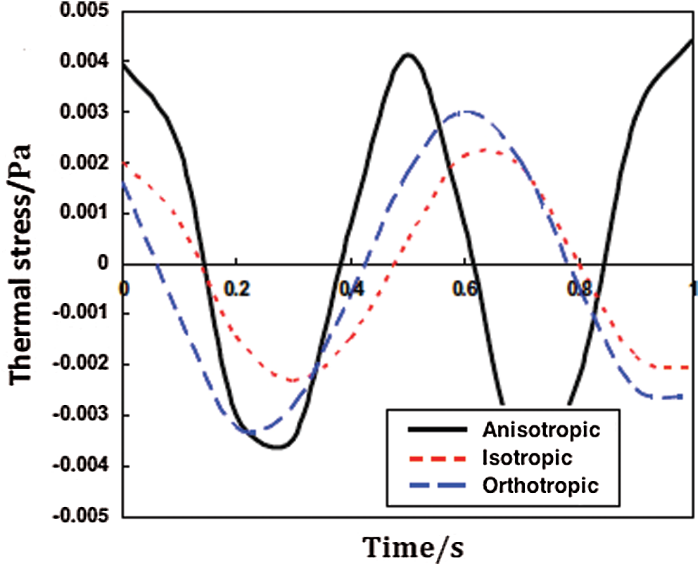
Figure 8: Propagation of the nonlinear thermal stress σ22 waves with time t for isotropic, orthotropic and anisotropic porous materials

Figs. 9–11 display the propagation of nonlinear thermal stress waves σ11, σ12, and σ22 for homogeneous (m = 0) and functionally graded (m=0.4 and 0.7) porous structures. It can be shown from these figures that the effect of functionally graded material is very pronounced.

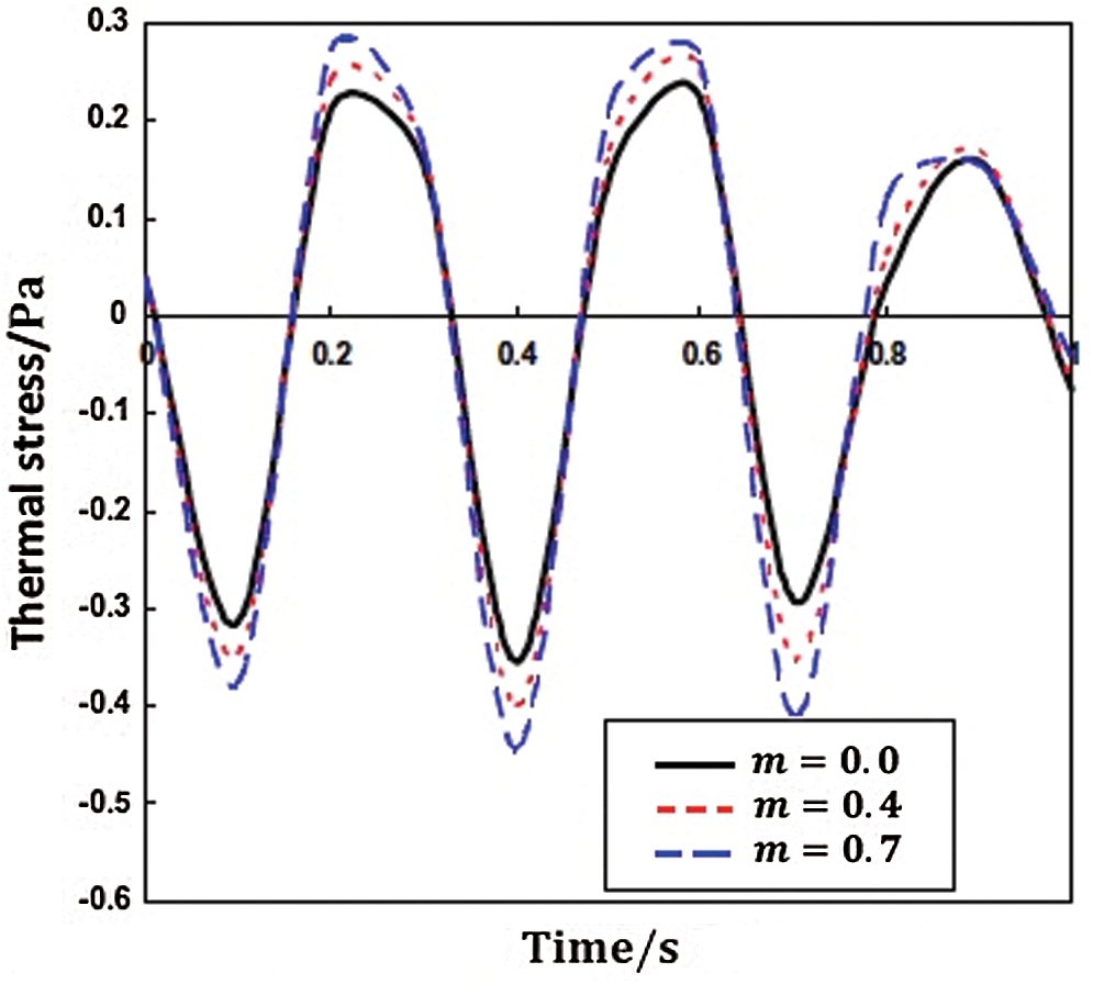
Figure 9: Propagation of the nonlinear thermal stress σ11 waves with time t for homogeneous and functionally graded porous materials

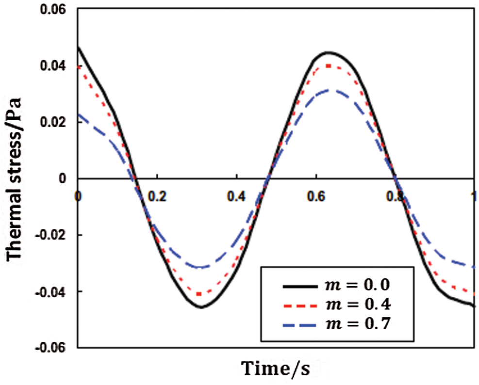
Figure 10: Propagation of the nonlinear thermal stress σ12 waves with time t for homogeneous and functionally graded porous materials

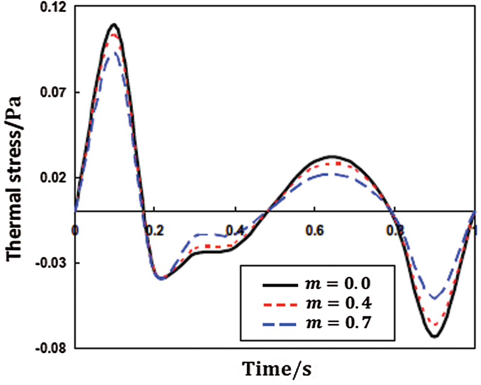
Figure 11: Propagation of the nonlinear thermal stress σ22 waves with time t for homogeneous and functionally graded porous materials

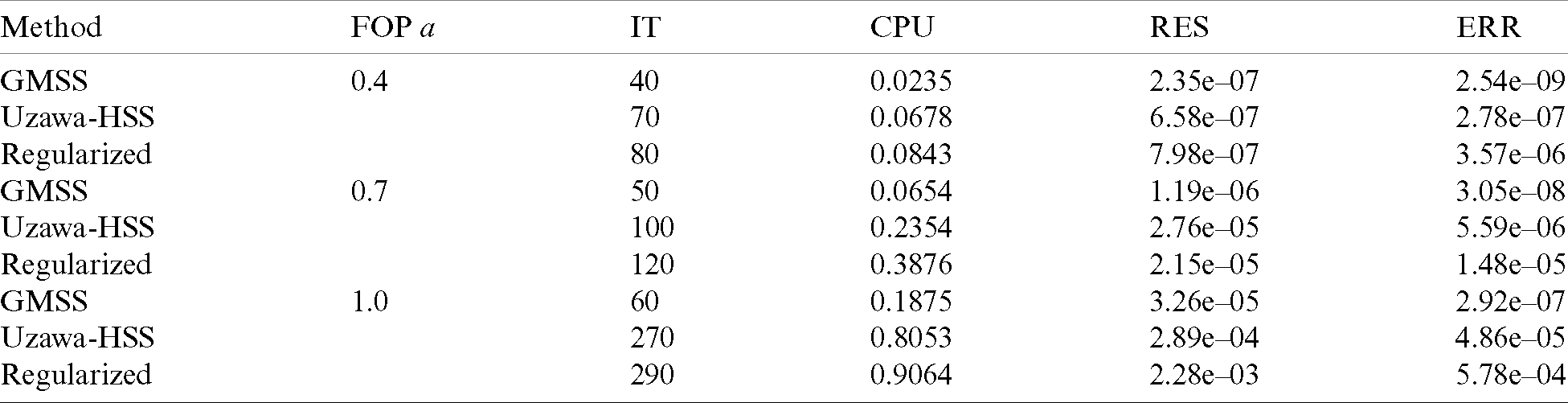
The effectiveness of our proposed approach has been established through the use of the GMSS which doesn’t need the entire matrix to be stored in the memory and converges quickly without the need for complicated calculations. During our treatment of the considered problem, we implemented GMSS, Uzawa-HSS, and regularized iteration methods [45]. Tab. 2 displays the number of iterations (IT), processor time (CPU), relative residual (RES), and error (ERR) of the considered methods computed for different fractional order values. It can be noted from Tab. 2 that the GMSS needs the lowest IT and CPU times, which means that GMSS method has better performance than Uzawa-HSS and regularized methods.

Table 2: Numerical results for the tested iteration methods

For comparison purposes with other methods, we only considered the one-dimensional special case. Therefore, the time distribution results of the nonlinear thermal stress σ11 are plotted in Fig. 12 for the proposed BEM and compared with the FDM results obtained by Awrejcewicz et al. [46] and FEM results obtained by Shakeriaski et al. [47], it can be shown from Fig. 12 that the BEM outcomes are in very good agreement with the FDM and FEM outcomes. Thus, the validity, accuracy, and usefulness of the proposed BEM have been demonstrated.

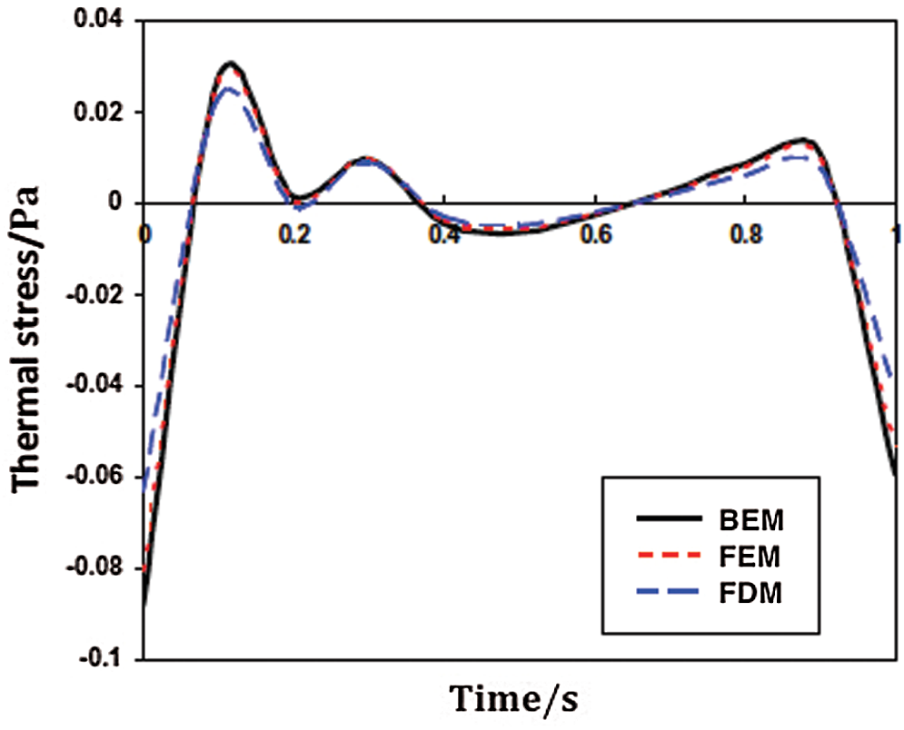
Figure 12: Propagation of the nonlinear thermal stress σ11 waves with time t for a special case and different methods

6  Conclusion

The main objective of the current paper is to develop a new boundary element model for solving fractional-order nonlinear generalized porothermoelastic wave propagation problems in FGA structures, which are difficult or impossible to solve analytically. Therefore, an efficient numerical procedure based on BEM has been proposed to overcome this challenge. The Kirchhoff transformation is first used to treat the nonlinear terms. Then, the Cartesian transformation method (CTM) has been applied to transform the domain integration into boundary integration, As a result, the computational complexity of integration and CPU computing time are significantly reduced. The memory requirements and Processing time are also reduced by applying the GMSS method which does not need that the entire matrix is stored in the memory, and it is rapidly converging without the need for complicated calculations. The numerical outcomes are presented graphically to show the effects of fractional parameter, anisotropy, and functionally graded material on the nonlinear thermal stress waves. The numerical outcomes also show very good agreement with the earlier work in the literature as a special case. These outcomes also confirm the validity, accuracy, and effectiveness of the proposed methodology.

Funding Statement: The author received no specific funding for this study.

Conflicts of Interest: The author declares that he has no conflicts of interest to report regarding the present study.

References

 1.  K. B. Oldham and J. Spanier. (2006). The Fractional Calculus: Theory and Applications of Differentiation and Integration to Arbitrary Order, 1st ed., vol. 111. Mineola, USA: Dover Publication, pp. 1–64. [Google Scholar]

 2.  R. L. Bagley and P. J. Torvik. (1986). “On the fractional calculus model of viscoelastic behavior,” Journal of Rheology, vol. 30, no. 1, pp. 133–155. [Google Scholar]

 3.  H. M. Ozaktas, O. Arikan, M. A. Kutay and G. Bozdagi. (1996). “Digital computation of the fractional Fourier transform,” IEEE Transactions on Signal Processing, vol. 44, no. 9, pp. 2141–2150. [Google Scholar]

 4.  J. A. T. Machado. (1997). “Analysis and design of fractional-order digital control systems,” SAMS Journal of Systems Analysis, Modelling and Simulation, vol. 27, no. 2–3, pp. 107–122. [Google Scholar]

 5.  A. A. Kilbas, H. M. Srivastava and J. J. Trujillo. (2006). Theory and Applications of Fractional Differential Equations, 1st ed., vol. 204. Amsterdam, The Netherlands: Elsevier Science, pp. 449–463. [Google Scholar]

 6.  J. Sabatier, O. P. Agrawal and J. A. T. Machado. (2007). Advances in Fractional Calculus: Theoretical Developments and Applications in Physics and Engineering, 1st ed., vol. 1. Dordrecht, The Netherlands: Springer, pp. 169–302. [Google Scholar]

 7.  M. D. Ortigueira, J. A. T. Machado and J. S. Da Costa. (2005). “Which differintegration? [fractional calculus],” IEE Proceedings—Vision, Image and Signal Processing, vol. 152, no. 6, 9, pp. 846–850. [Google Scholar]

 8.  K. Diethelm. (1997). “Generalized compound quadrature formulae for finite-part integrals,” IMA Jornal of Numerical Analysis, vol. 17, no. 3, pp. 479–493. [Google Scholar]

 9.  J. L. Wang and H. F. Li. (2011). “Surpassing the fractional derivative: concept of the memory-dependent derivative,” Computers and Mathematics with Applications, vol. 62, no. 3, pp. 1562–1567. [Google Scholar]

10. Y. J. Yu and L. J. Zhao. (2020). “Fractional thermoelasticity revisited with new definitions of fractional derivative,” European Journal of Mechanics—A/Solids, vol. 84, no. 11, 12, pp. 104043. [Google Scholar]

11. H. H. Sherief and M. A. Ezzat. (1994). “Solution of the generalized problem of thermoelasticity in the form of series of functions,” Journal of Thermal Stresses, vol. 17, no. 1, pp. 75–95. [Google Scholar]

12. M. A. Ezzat. (2004). “Fundamental solution in generalized magneto-thermoelasticity with two relaxation times for perfect conductor cylindrical region,” International Journal of Engineering Science, vol. 42, no. 13–14, pp. 1503–1519. [Google Scholar]

13. M. A. Fahmy. (2012). “The effect of rotation and inhomogeneity on the transient magneto-thermoviscoelastic stresses in an anisotropic solid,” ASME Journal of Applied Mechanics, vol. 79, no. 5, pp. 1015. [Google Scholar]

14. M. A. Ezzat and A. A. El-Bary. (2015). “Memory-dependent derivatives theory of thermo-viscoelasticity involving two-temperature,” Journal of Mechanical Science and Technology, vol. 29, no. 10, pp. 4273–4279. [Google Scholar]

15. S. M. Said. (2016). “Wave propagation in a magneto-micropolar thermoelastic medium with two temperatures for three-phase-lag model,” Computers, Materials & Continua, vol. 52, no. 1, pp. 1–24. [Google Scholar]

16. M. A. Ezzat and E. S. Awad. (2010). “Constitutive relations, uniqueness of solution, and thermal shock application in the linear theory of micropolar generalized thermoelasticity involving two temperatures,” Journal of Thermal Stresses, vol. 33, no. 3, pp. 226–250. [Google Scholar]

17. M. A. Fahmy. (2011). “A time-stepping DRBEM for magneto-thermo-viscoelastic interactions in a rotating nonhomogeneous anisotropic solid,” International Journal of Applied Mechanics, vol. 3, no. 4, pp. 1–24. [Google Scholar]

18. M. A. Fahmy. (2012). “A time-stepping DRBEM for the transient magneto-thermo-visco-elastic stresses in a rotating non-homogeneous anisotropic solid,” Engineering Analysis with Boundary Elements, vol. 36, no. 3, pp. 335–345. [Google Scholar]

19. C. A. Brebbia and S. Walker. (1980). Boundary Element Techniques in Engineering, 1st ed., vol. 1. Amsterdam, The Netherlands: Elsevier Science, pp. 151–179. [Google Scholar]

20. P. W. Partridge and C. A. Brebbia. (1990). “Computer implementation of the BEM dual reciprocity method for the solution of general field equations,” Communications in Applied Numerical Methods, vol. 6, no. 2, pp. 83–92. [Google Scholar]

21. M. A. Fahmy. (2018). “Shape design sensitivity and optimization of anisotropic functionally graded smart structures using bicubic B-splines DRBEM,” Engineering Analysis with Boundary Elements, vol. 87, no. 2, pp. 27–35. [Google Scholar]

22. M. A. Fahmy. (2018). “Shape design sensitivity and optimization for two-temperature generalized magneto-thermoelastic problems using time-domain DRBEM,” Journal of Thermal Stresses, vol. 41, no. 1, pp. 119–138. [Google Scholar]

23. M. A. Fahmy. (2018). “Boundary element algorithm for modeling and simulation of dual-phase lag bioheat transfer and biomechanics of anisotropic soft tissues,” International Journal of Applied Mechanics, vol. 10, no. 10, pp. 1850108. [Google Scholar]

24. M. A. Fahmy. (2019). “A new boundary element strategy for modeling and simulation of three temperatures nonlinear generalized micropolar-magneto-thermoelastic wave propagation problems in FGA structures,” Engineering Analysis with Boundary Elements, vol. 108, no. 11, pp. 192–200. [Google Scholar]

25. M. Mohammadi, M. R. Hematiyan and L. Marin. (2010). “Boundary element analysis of nonlinear transient heat conduction problems involving non-homogenous and nonlinear heat sources using time-dependent fundamental solutions,” Engineering Analysis with Boundary Elements, vol. 34, no. 7, pp. 655–665. [Google Scholar]

26. M. A. Fahmy. (2020). “Boundary element algorithm for nonlinear modeling and simulation of three-temperature anisotropic generalized micropolar piezothermoelasticity with memory-dependent derivative,” International Journal of Applied Mechanics, vol. 12, no. 3, pp. 2050027. [Google Scholar]

27. Y. C. Shiah, S. C. Huang and M. R. Hematiyan. (2020). “Efficient 2D analysis of interfacial thermoelastic stresses in multiply bonded anisotropic composites with thin adhesives,” Computers, Materials & Continua, vol. 64, no. 2, pp. 701–727. [Google Scholar]

28. F. Bayones, A. M. Abd-Alla, R. Alfatta and H. Al-Nefaie. (2020). “Propagation of a thermoelastic wave in a half-space of a homogeneous isotropic material subjected to the effect of rotation and initial stress,” Computers, Materials & Continua, vol. 62, no. 2, pp. 551–567. [Google Scholar]

29. G. Sowmya, B. J. Gireesha and M. Madhu. (2020). “Analysis of a fully wetted moving fin with temperature-dependent internal heat generation using the finite element method,” Heat Transfer, vol. 49, no. 4, pp. 1939–1954. [Google Scholar]

30. G. Sobamowo, B. Y. Ogunmola and G. C. Nzebuka. (2017). “Finite volume method for analysis of convective longitudinal fin with temperature-dependent thermal conductivity and internal heat generation,” Defect and Diffusion Forum, vol. 374, no. 4, pp. 106–120. [Google Scholar]

31. J. Gong, L. Xuan, B. Ying and H. Wang. (2019). “Thermoelastic analysis of functionally graded porous materials with temperature-dependent properties by a staggered finite volume method,” Composite Structures, vol. 224, no. 18, pp. 111071. [Google Scholar]

32. D. G. Dilip, G. John, S. Panda and J. Mathew. (2020). “Finite-volume-based conservative numerical scheme in cylindrical coordinate system to predict material removal during micro-EDM on Inconel 718,” Journal of the Brazilian Society of Mechanical Sciences and Engineering, vol. 42, no. 2, pp. 90. [Google Scholar]

33. R. Koprowski. (2020). Fractal Analysis-Selected Examples, London, UK: IntechOpen, pp. 56–85. [Google Scholar]

34. C. Cattaneo. (1958). Sur une forme de i’equation de la chaleur elinant le paradox d’une propagation instantanc, Comptes rendus de l’Académie des Sciences, vol. 247. Paris: Gauthier-Villars, pp. 431–433. [Google Scholar]

35. O. A. Ezekoye. (2016). Conduction of Heat in Solids, New York, USA: Springer. [Google Scholar]

36. L. C. Wrobel. (2002). The boundary Element Method: Applications in Thermo-Fluids and Acoustics, 1st ed., vol. 1. New York, USA: John Wiley & Sons, pp. 97–142. [Google Scholar]

37. M. R. Hematiyan. (2008). “Exact transformation of a wide variety of domain integrals into boundary integrals in boundary element method,” Communications in Numerical Methods in Engineering, vol. 24, no. 11, pp. 1497–1521. [Google Scholar]

38. M. R. Hematiyan. (2007). “A general method for evaluation of 2D and 3D domain integrals without domain discretization and its application in BEM,” Computational Mechanics, vol. 39, no. 4, pp. 509–520. [Google Scholar]

39. A. Khosravifard and M. R. Hematiyan. (2010). “A new method for meshless integration in 2D and 3D Galerkin meshfree methods,” Engineering Analysis with Boundary Elements, vol. 34, no. 1, pp. 30–40. [Google Scholar]

40. G. R. Liu and Y. T. Gu. (2005). An Introduction to Meshfree Methods and Their Programming, New York, USA: Springer. [Google Scholar]

41. M. Breuer, G. De Nayer, M. Münsch, T. Gallinger and R. Wüuchner et al. (2012). , “Fluid-structure interaction using a partitioned semi-implicit predictor-corrector coupling scheme for the application of large-eddy simulation,” Journal of Fluids and Structures, vol. 29, no. 2, pp. 107–130. [Google Scholar]

42. S. W. Zhou, A. L. Yang, Y. Dou and Y. J. Wu. (2016). “The generalized modified shift-splitting preconditioners for nonsymmetric saddle point problems,” Applied Mathematics Letters, vol. 59, no. 9, pp. 109–114. [Google Scholar]

43. D. Green and R. Perry. (2007). Perry’s Chemical Engineer’s Handbook, 7th ed., vol. 1. New York, USA: Mc Graw-Hill, pp. 2205–2233. [Google Scholar]

44. C. Lamuta. (2019). “Elastic constants determination of anisotropic materials by depth-sensing indentation,” SN Applied Sciences, vol. 1, no. 10, pp. 1263. [Google Scholar]

45. M. A. Fahmy. (2021). “A novel BEM for modeling and simulation of 3T nonlinear generalized anisotropic micropolar-thermoelasticity theory with memory dependent derivative,” Computer Modeling in Engineering & Sciences, vol. 126, no. 1, pp. 175–199. [Google Scholar]

46. J. Awrejcewicz and V. A. Krysko. (2020). Elastic and Thermoelastic Problems in Nonlinear Dynamics of Structural Members: Applications of the Bubnov-Galerkin and Finite Difference Methods, New York, USA: Springer International Publishing. [Google Scholar]

47. F. Shakeriaski and M. Ghodrat. (2020). “The nonlinear response of Cattaneo-type thermal loading of a laser pulse on a medium using the generalized thermoelastic model,” Theoretical and Applied Mechanics Letters, vol. 10, no. 4, pp. 1–12. [Google Scholar]

This work is licensed under a Creative Commons Attribution 4.0 International License, which permits unrestricted use, distribution, and reproduction in any medium, provided the original work is properly cited.