Computers, Materials & Continua DOI:10.32604/cmc.2021.014171
Article

Spatio-Temporal Dynamics and Structure Preserving Algorithm for Computer Virus Model

Nauman Ahmed1,2, Umbreen Fatima1, Shahzaib Iqbal1, Ali Raza3, Muhammad Rafiq4,*, Muhammad Aziz-ur-Rehman2, Shehla Saeed1, Ilyas Khan5 and Kottakkaran Sooppy Nisar6

1Department of Mathematics and Statistics, The University of Lahore, Lahore, Pakistan
2Department of Mathematics, University of Management and Technology, Lahore, Pakistan
3Department of Mathematics, National College of Business Administration and Economics, Lahore, Pakistan
4Department of Mathematics, Faculty of Sciences, University of Central Punjab, Lahore, Pakistan
5Faculty of Mathematics and Statistics, Ton Duc Thang University, Ho Chi Minh, 72915, Vietnam
6Department of Mathematics, College of Arts and Sciences at Wadi Aldawaser, Prince Sattam Bin Abdulaziz University, Alkharj, Saudi Arabia
*Corresponding Author: Muhammad Rafiq. Email: m.rafiq@ucp.edu.pk
Received: 03 September 2020; Accepted: 20 December 2020

Abstract: The present work is related to the numerical investigation of the spatio-temporal susceptible-latent-breaking out-recovered (SLBR) epidemic model. It describes the computer virus dynamics with vertical transmission via the internet. In these types of dynamics models, the absolute values of the state variables are the fundamental requirement that must be fulfilled by the numerical design. By taking into account this key property, the positivity preserving algorithm is designed to solve the underlying SLBR system. Since, the state variables associated with the phenomenon, represent the computer nodes, so they must take in absolute. Moreover, the continuous system (SLBR) acquires two steady states i.e., the virus-free state and the virus existence state. The stability of the numerical design, at the equilibrium points, portrays an exceptional aspect about the propagation of the virus. The designed discretization algorithm sustains the stability of both the steady states. The computer simulations also endorse that the proposed discretization algorithm retains all the traits of the continuous SLBR model with spatial content. The stability and consistency of the proposed algorithm are verified, mathematically. All the facts are also ascertained by numerical simulations.

Keywords: Spatio-temporal; computer virus model; discretization; positive solution; computer simulations

1  Introduction

A computer virus is a program that can be spread out among the computers and networks by replicating itself. These viruses are deleterious for computer software as well as hardware. The message of removing all the files on your system is a clear indication of the virus attack. The virus can reproduce itself by operating on some other programs like an epidemic disease [1]. The motive behind developing the malware is to contaminate the systems, destruction of computer hardware, and stealing of significant data. In this way, the hackers get administrative control of the system [2]. They design such viruses with the malevolent intention to victimize online users by setting a trap for them. A virus infects the computer when malware runs on the system. They use many techniques to make the program run by the user. When someone opens the file, the virus attaches to it or hides in the form of codes that runs, automatically. When someone receives an infected file by email or from the internet while downloading the other files and the virus code becomes active, when the file is opened. In this way, the virus can make replicas of itself on a computer disk, on other files and can change the setting of the computers. Boot sector virus, direct action virus, resident virus, parasitic virus (file virus), multipartite virus, polymorphic virus, and macro viruses are some of the common computer viruses. The viruses not only corrupt or remove the data but can also harm the economy by interrupting trade activities. It is a common fact about the viruses that they can remove or corrupt everything on the hard drive. This is a serious issue, but a strong backup can resolve this problem. Some side-effects are more serious, for instance during working hours the virus prevents systems from functioning and gives a shutdown command to the device, resulting in economic loss. Some viruses interrupt the business activities, for instance, Melissa or Explore Zip, can block or destroy the server by generating a lot of unnecessary emails. Sometimes companies detect and respond to the risk by shutting down their mail servers to avoid the situation. When a system becomes infected, it shows unusual behavior such as low performance, automatic multiplication of the files, and the self-running of the program files, etc. Moreover, the files and folders become corrupted and the hard disk produces sounds. Now, people can get information more quickly than ever before, by the internet. The pitfall that has also arisen, is the harmful computer codes, which access the systems by different modes. The risk of virus spread has increased by the use of the internet and it is a major threat to internet users [3]. In the recent past, most of the viruses were propagated by floppy or compact disks. So, the role of the user in spreading the virus was obvious. Moreover, the side effects of the virus were so clear that everyone could adopt safety and precautionary measures. Now, the extensive use of the internet has changed the scenario by rapid sharing of the software. So, the propagation of any virus via the internet is very easy. Anyone can download a program easily from a website. So, the parasitic (file) viruses can rapidly grow by the widespread usage of the net. The micro viruses can seriously affect the documents. The internet users download the documents, spreadsheets, or files in routine and exchange them by email. A computer is infected either by downloading the file or by email. A computer virus works in two ways, the first one is instant replication when it runs on a susceptible computer and the second one remains inactive. In other words, the infected program needs to be run for its activation. Consequently, it is highly important to stay protected from viruses by installing a robust antivirus program. Only the end-users of the internet are safe. Some hackers make websites for targeting web servers. It is a common strategy to send a large number of requests on the webserver which slow down or crash it. When this happens, the candid user can no longer be able to get access to the website which is hosted by the server. It is worth mentioning that malicious computer viruses have become a great peril to the community. Since they acquire data and damage the parts of the computer like the hard drive and motherboard. To understand the dynamics of the computer virus, the mathematical epidemic models play an imperative role [4–9]. Numerous researchers suggested different mathematical models for explaining the virus communication through different mediums [10–14]. Here, the spatially-structured computer virus model is studied analytically and numerically [15,16].

∂S∂t=μ-μS-βS(L+B)+α(1-S-L-B)+ds∂2S∂x2 (1)

∂L∂t=βS(L+B)-μL-ϵL+dL∂2L∂x2 (2)

∂B∂t=ϵL-μB-γB+dB∂2B∂x2

The initial conditions are of the form

S(x,0)=Φ1(x)≥0,L(x,0)=Φ2(x)≥0,B(x,0)=Φ3(x)≥0,0≤x≤L(3)

and the boundary conditions are

∂S(0,t)∂x=∂L(0,t)∂x=∂B(0,t)∂x=0;t>0,∂S(L,t)∂x=∂L(L,t)∂x=∂B(L,t)∂x=0;t>0,

Also, S+L+B≤1.

Here, the quantity S describes the susceptible computers at time t and space x, that can be infected from virus, L and B represent the latent and the breaking out computers at time t and space x. The parameter μ is the rate at which the computers are connected and withdrawn from the internet. The parameters β, γ and ϵ are transmission rate, recovery rate and latent to breaking out rate respectively. The nonnegative constant value of α is the rate at which recovered computers become susceptible again. This study is about the numerical investigation of the computer virus epidemic model with diffusion in one space dimension. The motive behind this study is to design a reliable numerical algorithm that preserves all the core structure of the continuous computer virus epidemic model. In the literature, various researchers have designed many structure-preserving numerical techniques and applied them to solve the various dynamical systems belonging to different areas of science and engineering [17–21]. The appearance of chaotic behavior in graphical solutions by using a numerical technique whereas this chaos is not the part of the physical system under study is called the contrived chaos. The algorithm proposed in this manuscript not only eliminates this type of contrived chaos but also retains the positive behavior of the solution to the model (1)–(3).

2  Steady States of the System

This section is meant for the steady states of the model. The steady states of a dynamical system have a decisive role in describing the stability of the system as well as of the algorithm. There are two states of the computer virus epidemic model, virus-free state (VFS) and virus persistence state (VPS). VFS is E1=(S0,L0,B0)=(1,0,0).

VPS is

E1=(S*,L*,B*)=((γ+μ)(μ+ε)β(μ+γ+ε),(γ+μ)(μ+α)β(μ+γ+ε)-(γ+μ)(γ+μ)(μ+ε)(μ+α)β(μ+γ+ε)(α+μ+ε)(γ+μ)+αε,ε(1-γ-μ)[(γ+μ)(μ+α)β(μ+γ+ε)-(γ+μ)(γ+μ)(μ+ε)(μ+α)β(μ+γ+ε)(α+μ+ε)(γ+μ)+αε]).

ℜ*=β(μ+γ+ε)(μ+ε)(μ+γ), where dS = dL = dB = 0. ℜ* is the basic reproductive value of underlying system (1)–(3).

3  Numerical Methods

In this portion, the proposed numerical design will be presented. To construct the algorithm, we divide [0,L]×[0,T] into M×N, with step sizes Δx=LM and Δt=TN. The nodal points for both the domains i.e., space and time, are considered as,

xn=nΔx,n∈{0,1,…,M},tj=jδt,j∈{0,1,…,N}.

Snj, Lnj and Bnj denote the FD approximations of S(nΔx,jΔt),L(nΔx,jΔt) and B(nΔx,jΔt) respectively.

Now, the proposed FD scheme for (3) is developed on the basis of the rules presented by Micken [22] as follows;

Snj+1=Snj+R1(Sn-1j+Sn+1j)-2R1Snj+1+Δtμ-Δtβ(Lnj+Bnj)Snj+1-ΔtμSnj+1+αΔt(1-Snj-Lnj-Bnj)(4)

After some computations, we have

Snj+1=Snj+R1(Sn-1j+Sn+1j)+μΔt+αΔt(1-Snj-Lnj-Bnj)1+2R1+Δtμ+Δtβ(Lnj+Bnj)(5)

In a similar way, we have

Lnj+1=Lnj+R2(Ln-1j+Ln+1j)+Δtβ(Lnj+Bnj)Snj1+2R2+Δt(μ+ϵ)(6)

and

Bnj+1=Bnj+R3(Bn-1j+Bn+1j)+ΔtϵLnj1+2R3+Δt(μ+γ)(7)

Here, R1=dSΔtΔx2, R2=dEΔtδx2 and R3=dIΔtΔx2.

4  Stability of the Proposed Scheme

This section is devoted to validate the stability of the proposed algorithm (5)–(7) by using Von Neumann stability criteria.

Theorem: The proposed algorithm (5)–(7) is Von Neumann stable.

Proof. Substituting Snj=η(t)eiζx in the proposed algorithm (4) and then linearizing, we have

η(t+δt)eiζx=η(t)eiζx+R1(eiζ(x-δx)+eiζ(x+δx))η(t)-2R1η(t+δt)eiζx-μΔtη(t+δt)eiζx-βδtη(t+Δt)

After some computations, we have,

|η(t+Δt)η(t)|=|1+2R1-4R1sin2(ζΔx/2)1+2R1+Δtμ+βΔt|≤|1-2R11+2R1+Δtμ+βΔt|<1

From the above expression, it is clear that the approximation algorithm (5) is Von Neumann stable. In a similar fashion, it can be observed that the approximate algorithms (6) and (7) are also Von Neumann stable.

5  Consistency of the Proposed Scheme

In this section, we verify that the proposed algorithms (5)–(7) are consistent. For this, we apply the Taylor series expansion on Snj+1, Sn+1j and Sn-1j as follows:

Snj+1=Snj+Δt∂S∂t+Δt22!∂2S∂t2+Δt33!∂3S∂t3+⋯Sn+1j=Snj+Δx∂S∂x+Δx22!∂2S∂x2+Δx33!∂3S∂x3+⋯Sn-1j=Snj-Δx∂S∂x+Δx22!∂2S∂x2-Δx33!∂3S∂x3+⋯

First, we consider the finite difference approximation algorithm (4) for the consistency of the proposed numerical scheme,

Snj+1=Snj+R1(Sn-1j+Sn+1j)-2R1Snj+1+Δtμ-Δtβ(Lnj+Bnj)Snj+1-ΔtμSnj+1+αΔt(1-Snj-Lnj-Bnj)

Inserting the values of Snj+1,Sn+1j and Sn-1j in the above equation and simplifying the expression we have,

(∂S∂t+Δt2!∂2S∂t2+Δt23!∂3S∂t3+…)(1+dSΔtΔx2+Δtμ+Δtβ(Lnj+Bnj))=2dS(12!∂2S∂x2+Δx24!∂4S∂x4+⋯)+μ-β(Lnj+Bnj)Snj-μSnj+α(1-Snj-Lnj-Bnj)

After inserting Δt=Δx3 and Δx→0, the above equation coincides with (1). The similar procedure can be adopted to show that the finite difference approximation algorithms (6) and (7) are consistent.

6  Positivity of the Scheme

In this section, we present a result which shows that the proposed algorithm unconditionally retains the positivity of the computer virus model.

Theorem: The proposed algorithms (5)–(7) provide the positive solutions which are exhibited by the continuous system (1)–(3) under the non-negative initial functions ϕi, i = 1, 2, 3.

Proof: It is clear that the values ϕi≥0, ∀i∈{1,2,3} with S+L+B≤1. Also, no negative term is associated on the right hand side of algorithms (5)–(7). This proves the theorem.

7  Numerical Experiment

The following values of parameters [15,16] are used in numerical experiments.

7.1 Experiment 1

In the first experiment, the following initial conditions are supposed.

S(x,0)={0.2x,0≤x<0.50.2(1-x),0.5≤x≤1L(x,0)={0.4x,0≤x<0.50.4(1-x),0.5≤x≤1B(x,0)={0.3x,0≤x<0.50.3(1-x),0.5≤x≤1

From Fig. 1 it can be noticed that the maximum number of susceptible computers, latent computers, and infected computers are concentrated at the center of the domain value [0,1] and decreases linearly to zero at the corners x = 0 and x = 1.

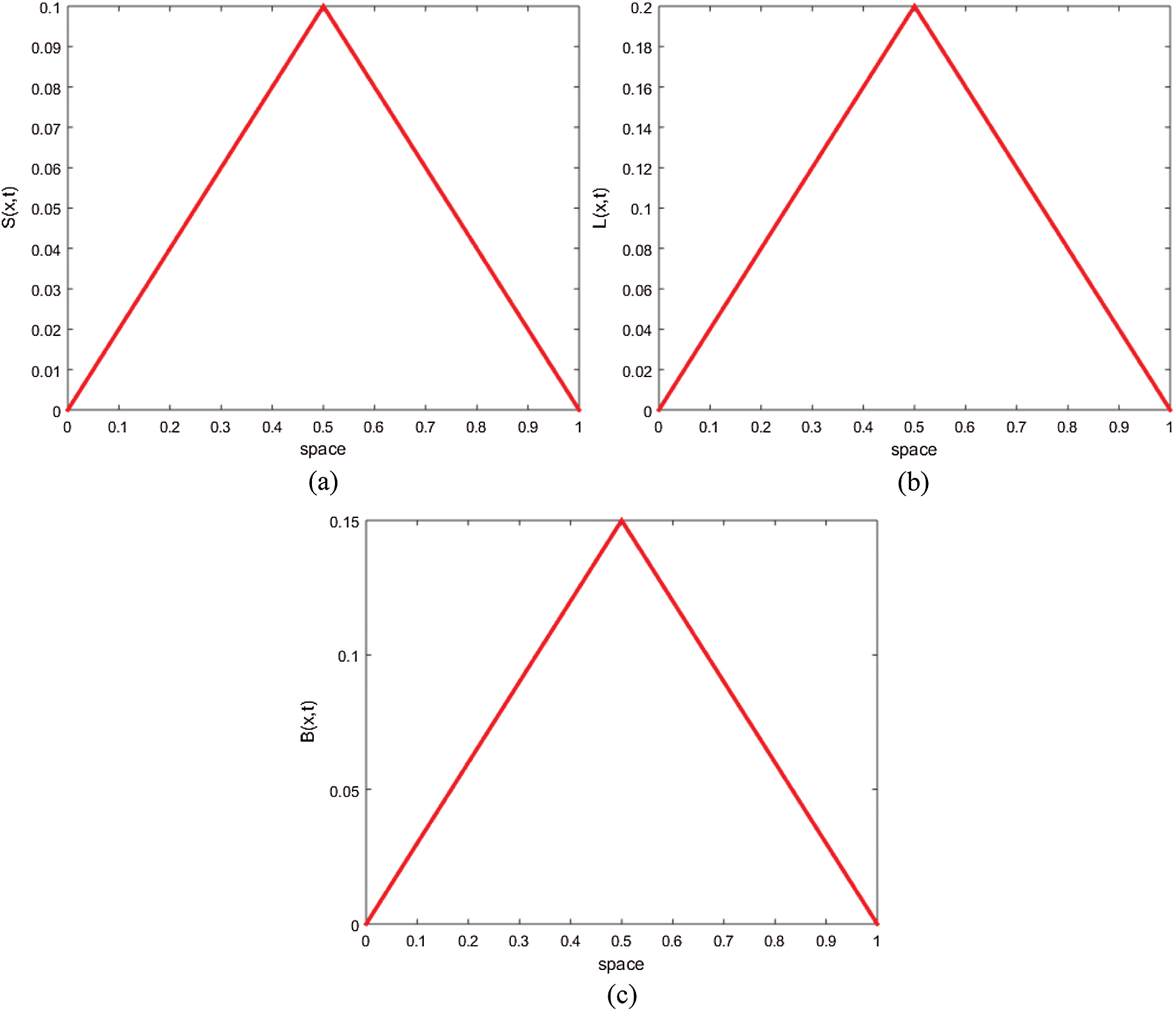
Figure 1: The initial dispersion of (a) susceptible computers, (b) latent computers and (c) breaking out computers

7.2 Disease Free Equilibrium

In this part, the graphical solutions of the proposed algorithm are examined against the parametric values taken in such a way that the value 𝔑cv is less than one i.e., virus free state.

In Fig. 2 we consider the values of the parameters describing VFS as mentioned in Tab. 1. The graphical representations reveal that the proposed algorithm demonstrates the positive behavior of the state variables S, L and B. Also, the algorithm under discussion attains the stability of VFS as these graphs converge to (1, 0, 0).

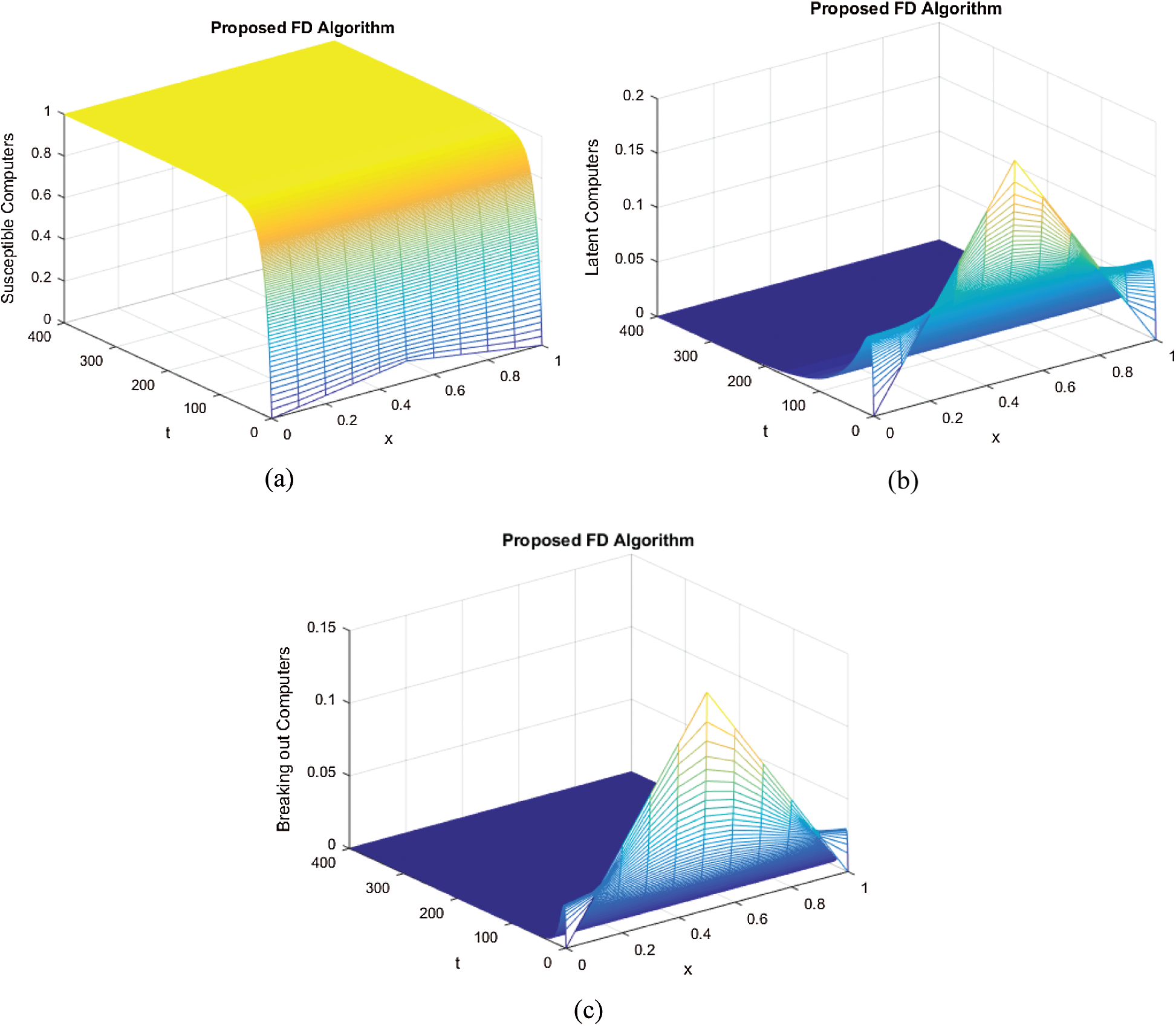
Figure 2: The graphical representation of (a) susceptible class of computers, (b) latent class of computers, (c) breaking out class of computers

Table 1: Parameters values

7.3 Endemic Equilibrium

This section is devoted to perform the graphical solutions of the proposed algorithm against the values that make 𝔑cv is greater than one i.e., virus persistence state.

Fig. 3 elaborates the solution behavior of S(x,t), L(x, t) and B(x, t) using designed algorithm for the state when virus exists in the computer population. Again, the computer simulations illustrate that the designed algorithm holds all the important properties of the SLBR model under discussion.

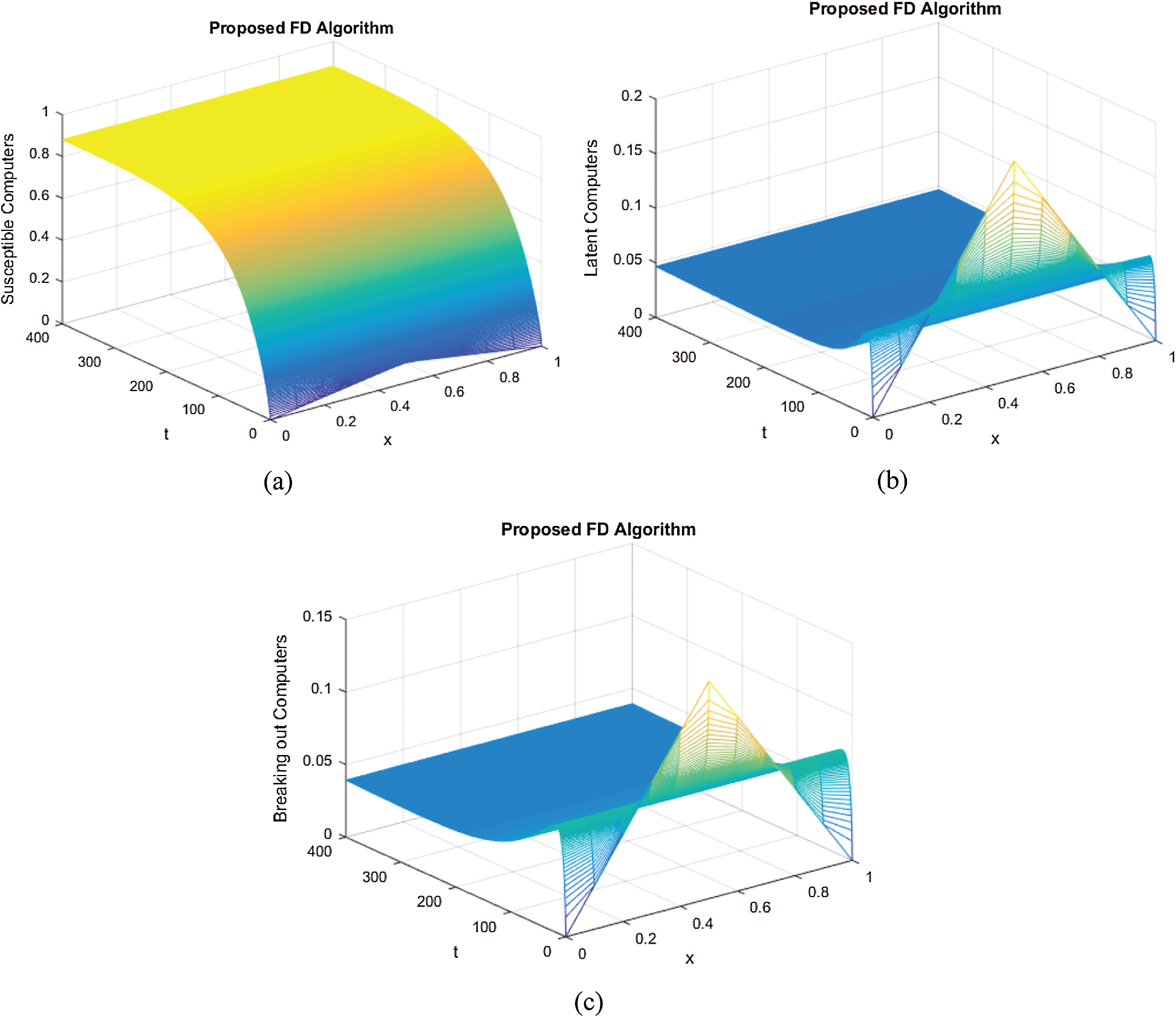
Figure 3: The graphical representation of (a) susceptible class of computers, (b) latent class of computers, (c) breaking out class of computers

8  Conclusion

The spatio-temporal computer virus epidemic model is proposed and studied, numerically. The algorithm proposed for the SLBR model is developed with the aid of the rules developed by Mickens. The consistency and the stability of the designed algorithm are confirmed with the Taylor series expansion and the Von Neumann criteria. The unknown variables of the SLBR model exhibit the computer population, so it is the basic property of the solutions to be positive. A theorem is presented which verifies that the underlying algorithm preserves positivity. The computer simulations demonstrate that the proposed numerical algorithm describes the consistent behavior with the continuous SLBR system. In the future, the current algorithm may be applied to solve the multidimensional reaction-diffusion systems. Furthermore, this numerical scheme may be applied to epidemic reaction-diffusion systems with time delay and predator-prey models with spatial content.

Funding Statement: The author(s) received no specific funding for this study.

Conflicts of Interest: The authors declare that they have no conflicts of interest to report regarding the present study.

This work is licensed under a Creative Commons Attribution 4.0 International License, which permits unrestricted use, distribution, and reproduction in any medium, provided the original work is properly cited.