DOI:10.32604/cmc.2021.012431
| Computers, Materials & Continua DOI:10.32604/cmc.2021.012431 | |
| Article |
Paddy Leaf Disease Detection Using an Optimized Deep Neural Network
1Department of Computer Science & Engineering, University College of Engineering, BIT Campus, Anna University, Tiruchirappalli, 620024, India
2School of Computing, SRM Institute of Science and Technology, Kattankulathur, 603203, India
3Department of Electronics and Communication Engineering, University College of Engineering, BIT Campus, Anna University, Tiruchirappalli, 620024, India
4Department of Electronics & Communication Engineering, SSM Institute of Engineering and Technology, Dindigul, 624002, India
5Department of Mechanical Engineering, Rohini College of Engineering and Technology, Palkulam, 629401, India
6Department of ECE, Karpagam Academy of Higher Education, Coimbatore, 641021, India
7Department of Electrical and Electronics Engineering, SRM Institute of Science and Technology, Chennai, 603203, India
*Corresponding Author: Shankarnarayanan Nalini. Email: autnalini@gmail.com
Received: 30 August 2020; Accepted: 04 February 2021
Abstract: Precision Agriculture is a concept of farm management which makes use of IoT and networking concepts to improve the crop. Plant diseases are one of the underlying causes in the decrease in the number of quantity and quality of the farming crops. Recognition of diseases from the plant images is an active research topic which makes use of machine learning (ML) approaches. A novel deep neural network (DNN) classification model is proposed for the identification of paddy leaf disease using plant image data. Classification errors were minimized by optimizing weights and biases in the DNN model using a crow search algorithm (CSA) during both the standard pre-training and fine-tuning processes. This DNN-CSA architecture enables the use of simplistic statistical learning techniques with a decreased computational workload, ensuring high classification accuracy. Paddy leaf images were first preprocessed, and the areas indicative of disease were initially extracted using a k-means clustering method. Thresholding was then applied to eliminate regions not indicative of disease. Next, a set of features were extracted from the previously isolated diseased regions. Finally, the classification accuracy and efficiency of the proposed DNN-CSA model were verified experimentally and shown to be superior to a support vector machine with multiple cross-fold validations.
Keywords: Leaf classification; paddy leaf; deep learning; metaheuristics optimization; crow search algorithm
The early identification of plant disease indicators is of significant agricultural benefit. However, this task remains challenging due to a lack of embedded computer vision techniques designed for agricultural applications. Agricultural yields are also subject to multiple challenges, such as insufficient water and plant disease [1]. The early detection, treatment, and prevention of plant diseases, particularly in the early stages of onset, is thus an essential activity for increasing production [2]. However, few studies have addressed the issues associated with the efficient early-stage identification and classification of plant diseases, which are subject to strict limitations. For example, the manual examination of plants for this purpose is infeasible, as it is considerably time consuming and labor intensive. This has led to the application of image-processing methods for disease identification and prediction, based on the physical appearance of plant leaves [3]. These techniques have been applied to common rice plant diseases, including sheath rot, leaf blast, leaf smut, brown spot, and bacterial blight [4]. Image processing relies on segmentation results for the extraction of characteristic disease features, such as color, size, and shape [5]. However, efforts to then classify these features as specific disease types are complicated by extensive variations in plant symptoms. A single disease may manifest as yellow structures in some cases and brown in others [6]. A disease may also produce identical shapes and colors in a specific plant type, while others may produce similar colors but different shapes. While experts can readily classify plant diseases based on images, manual identification is far too time consuming and cost prohibitive to offer solutions for large-scale agriculture [7]. In addition, manual inspection is often inconsistent as it depends heavily on personal bias and experience [8]. As such, existing disease examination procedures often lead to inaccurate classification results, which have limited rice yields in the last few decades [9].
These issues have been addressed in recent years through the application of accurate and robust disease detection systems based on machine learning (ML). For example, Lu et al. [10] applied a deep convolution neural network (DCNN) to predicting paddy leaf diseases using a dataset comprised of 500 images of both normal and diseased stems and leaves. Ten common rice diseases were included in the classification task. Experimental results from studies using deep learning (DL) have exhibited increased disease classification accuracy, compared to the levels achieved by conventional ML techniques. Image classification often utilizes region of interest (ROI) estimation, a segmentation approach that relies on neutrosophic logic, preferably expanded from a fuzzy set, as described by Dhingra et al. [11]. This approach has been applied to three-membership functions in various segmentation tasks. Feature subsets are typically used for detecting affected plant leaves with reference to segmented sites. The random forest algorithm has also been shown to be effective in distinguishing diseased and healthy leaves.
Nidhis et al. [12] introduced a framework for predicting paddy leaf diseases based on the application of image-processing models, in which the severity of the disease was determined by calculating the spatial range of affected regions. This enabled the application of appropriate insect repellents in suitable quantities, to reduce bacterial blights, brown spots, and rice blast effects in paddy crops. Islam et al. [13] developed a novel image processing model that used red-green-blue (RGB) images of rice leaves to detect and classify rice plant diseases. Classification was then performed using a simple and effective naive Bayes (NB) classifier. Similarly, Devi et al. [14] applied image processing to diseased regions of rice leaves using a hybridized graylevel co-occurrence matrix (GLCM), a discrete wavelet transform (DWT), and the scan investigate filter target (SIFT) model. Diverse classifiers, such as multiclass support vector machines (SVMs), NBs, backpropagation neural networks, and the k-nearest neighbor algorithm have also been applied to classifying image regions as normal or diseased, based on extracted features. Santos et al. [15] developed a DCNN to identify and categorize weeds present in soybean images, based on a database composed of soil, soybean, broadleaf, and grass weed images. Kaya et al. [16] examined simulation outcomes from four diverse transfer learning techniques, used for plant classification, with a deep neural network (DNN) trained by four common datasets. The results demonstrated that transfer learning improved the accuracy of conventional ML models.
This study proposes a novel DNNfor paddy leaf disease classification. The error was minimized by optimizing weights and biases using a crow search algorithm (CSA), a metaheuristic search technique that mimics the behavior of crows. Optimization was conducted during both the standard pre-training and fine-tuning steps, to establish a DNN-CSA architecture that enables the use of simplistic statistical learning, thereby decreasing computational workload and ensuring high classification accuracy. Paddy leaf images were first preprocessed and areas indicative of disease were extracted using a k-means clustering model. Thresholding was then applied to eliminate healthy regions. Next, a set of features, including color, texture, and shape were extracted from previously isolated diseased regions. Finally, the proposed model was used to classify paddy leaf diseases. Results showed the DNN-CSA was superior to an SVM algorithm under multiple cross-fold validation.
The workflow for the proposed rice plant disease identification and classification technique is illustrated in Fig. 1. The individual steps are discussed in detail below.
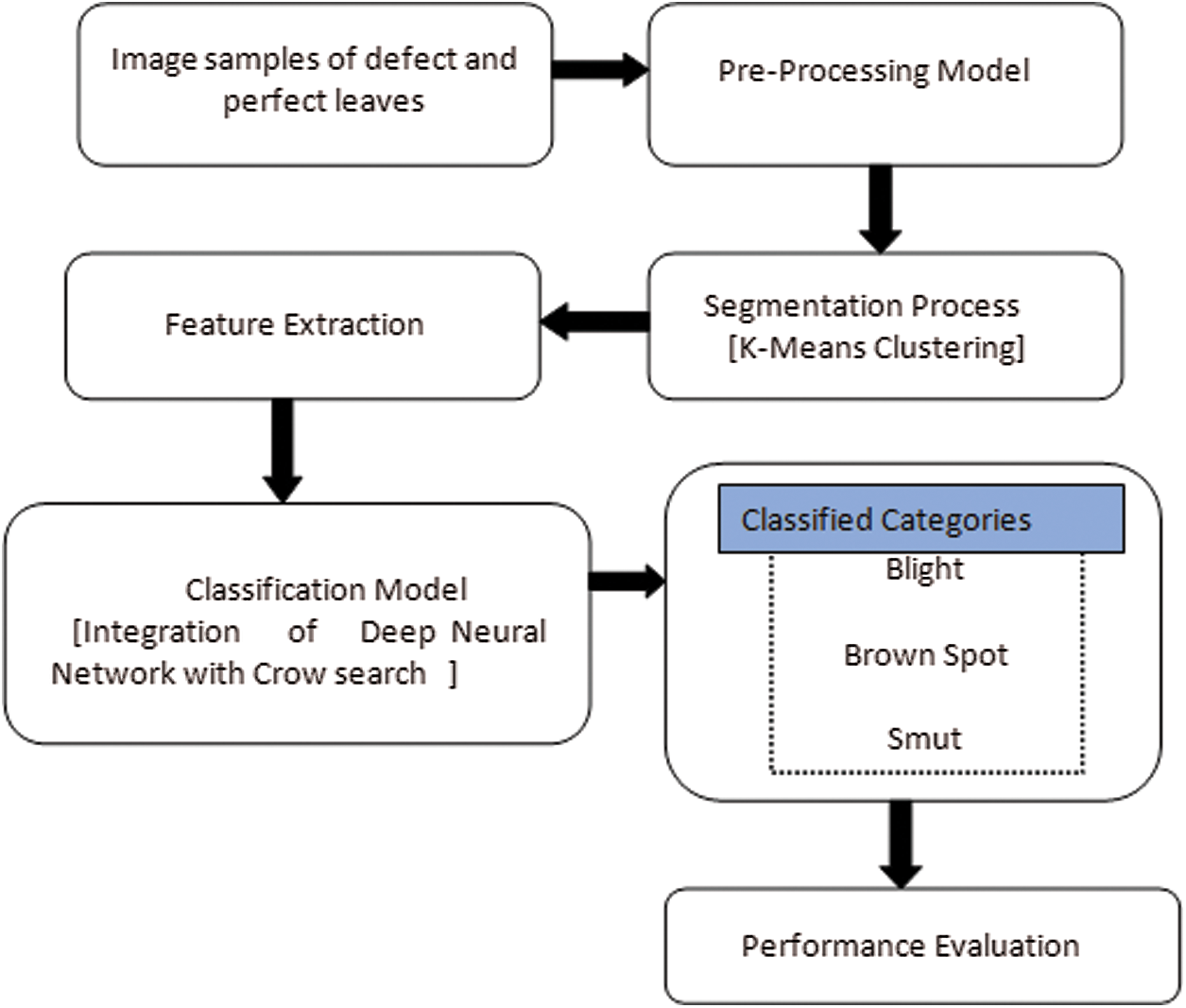
Figure 1: System design process of the proposed DNN-CS model
In real-time applications, photographs of rice plant leaves are collected using a high-resolution digital camera. A dataset containing images of both normal and diseased leaves was used in the analysis process [17]. These data were further divided into training (including ds1 and ds2) and testing sets.
Images in the dataset were scaled to a uniform size of
2.3 K-Means Clustering-Based Segmentation
Diseased regions in the background-eliminated HSV images were detected as clusters using a k-means clustering algorithm based solely on hue. The centroid value was used to make accurate segments for resolving randomness issues by constructing a histogram of hue components. Next, a specific threshold was identified from bin values in the hue histogram and used to distinguish between diseased clusters and normal regions in the image. Maximum hue values in each region were acquired from an appropriately selected cluster centroid. The rates of black colors and chosen centroid values were provided in the clustering step. Diseased regions produced in this process often included irregular regions of green pixels, which affected classification accuracy. Therefore, these irregular regions needed to be removed from the clustered sections. In the hue technique, green colors were mapped to a parameter with both lower and higher values.
Colors were also used to define shape and texture. The mean values of color, shape, and texture features were determined from the non-zero pixels in the RGB images, which represented the non-background regions of an image.
2.4.1 Extraction of Color Features
Diseased regions were defined using 14 colors. Initially, the color extraction process filtered regions of the RGB images that included diseased areas. The mean2 function in MATLAB was then applied after completion of the feature extraction process. The mean values of HSV components in the images were then identified. Finally, the std2 function in MATLAB was applied to the RGB color components.
2.4.2 Extraction of Shape Features
Shape features extracted from binary images acquired during preprocessing were based on irregularly shaped diseased regions (blobs) in the images. These blobs were generally used to detect image areas that represented different objects. Determining the number of diseased sections is therefore a critical component of the blob prediction approach.
2.4.3 Extraction of Texture Features
A GLCM was used to extract texture features from images. The GLCM records the number of times a pixel with a given gray level i is found to be horizontally adjacent to a pixel with a different gray level j, determined using the graycomatrix function in MATLAB. The GLCM used in this study was an
2.5 Deep Learning-Based Classification
The DNN architecture is composed of an input layer consisting of N input neurons (units), three layers of hidden units, and an output layer that provides classification results [18]. The DNN was trained using a DL technique composed of two stages: a pre-training step and a fine-tuning step. In the pre-training process, network weights were randomly initialized, and the model was trained using the training set. A fine-tuning model was then used to determine how well the model could be generalized to different plant species datasets. For this purpose, the training images were divided into two sets denoted as ds1 and ds2. This process is described in detail in the following sections.
In the pre-training step, the deep belief network (DBN) is applied to the input layer of the DNN, which is subsequently forwarded through hidden layers to the output layer, thereby assigning parameters for the activation functions employed in the individual nodes of the network. The assignment of activation function parameters was further performed by a restricted Boltzmann machine (RBM) using the following procedure. The elements of V(visible unit) are uploaded and used for training the RBM vector. A mutual configuration of (v,h) then produces the energy F(v,h) as follows:
Here, v is a visible unit, h is a hidden unit, Wpq represents the weights between a visible unit vp and a hidden unit hq (in the network),
Here,
where
The fine-tuning of network weights was conducted using back propagation (BP), which was applied using the network weights acquired from the pre-training phase. The improved network weights were obtained in the training phase using the training data once a minimum error rate was achieved.
Crows often monitor locations where neighboring birds hide food and will often steal food when competitors leave the immediate area. In addition, crows make use of this information to identify pilfering behavior in other birds and devise safeguarding measures to conceal food by varying hiding locations [19]. The CSA invokes these same strategies as follows:
• Crows move in a flock comprised of N crows;
• Crows remember their food concealment locations;
• Crows follow each other in the execution of a theft.
The CSA involves a metaheuristic search conducted in a d-dimensional space, where d denotes the number of decision variables. The location of crow u (
Suppose crow v moves to hiding place mvitr at iteration itr and crow u follows crow v to locate mvitr. In this case, the following two states must be considered.
State 1: Crow v is unaware of the pursuit activities of crow u. Consequently, crow u freely visits mvitr. The new position of crow u at iteration
where ru denotes an arbitrary value evenly distributed in the range [0, 1] and flu, itr represents the flight length of crow u along the vector [mv, itr − xu, itr]T at iteration itr. Here, small values of flu, itr correspond to local searches in the vicinity of xu, itr and large values correspond to global searches, typically far from xu, itr. As such, a value of flu, itr less than 1 represents a final destination between positions xu, itr and mv, itr, while a value of flu, itr greater than 1 represents a final destination on the side of mv, itropposite from xu, itr.
State 2: Crow v is aware of being followed by crow u and crow v misdirects crow u by travelling randomly to an alternate location in the search space.
States 1 and 2 are determined by the level of awareness rv of crow v at iteration itr, which is defined as an arbitrary value evenly distributed in the range [0, 1]. Therefore, xu, itr+1 is defined for both states by the following relationship:
Here, APv, itr is the awareness probability of crow v at iteration itr. The primary objective of the CSA is to determine optimal values of all d decision variables. A step-by-step procedure for CSA execution is provided below.
Step 1: Define parameters for the search process, including d, N, itrmx, and AP values.
Step 2: Initializethe positions of hidden food caches (in memory) for individual crows.
Step 3: Define the objective function
Step 4: Evaluate the relative fitness of a hidden food cache location for every crow in the flock.
Decision variables are evaluated by introducing the locations stored in memory into the objective function. These locations are defined for each of the N crows and each of the d decision variables as follows:
Step 5: Generatenovel hidden food cache locations (in the search space) for all crows in the flock, using the process outlined in Eq. (5).
Step 6: The fitness function is used to measure the quality of solutions provided by a search agent. Determine the fitness functionf(x
Step 7: Upgrade the elements of Memory at iteration
Step 8: Repeat Steps 5–7 until
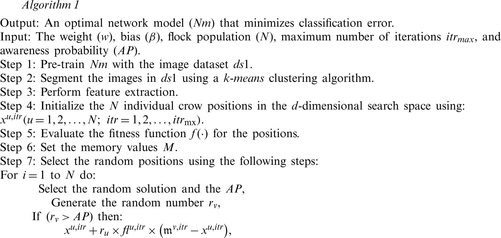
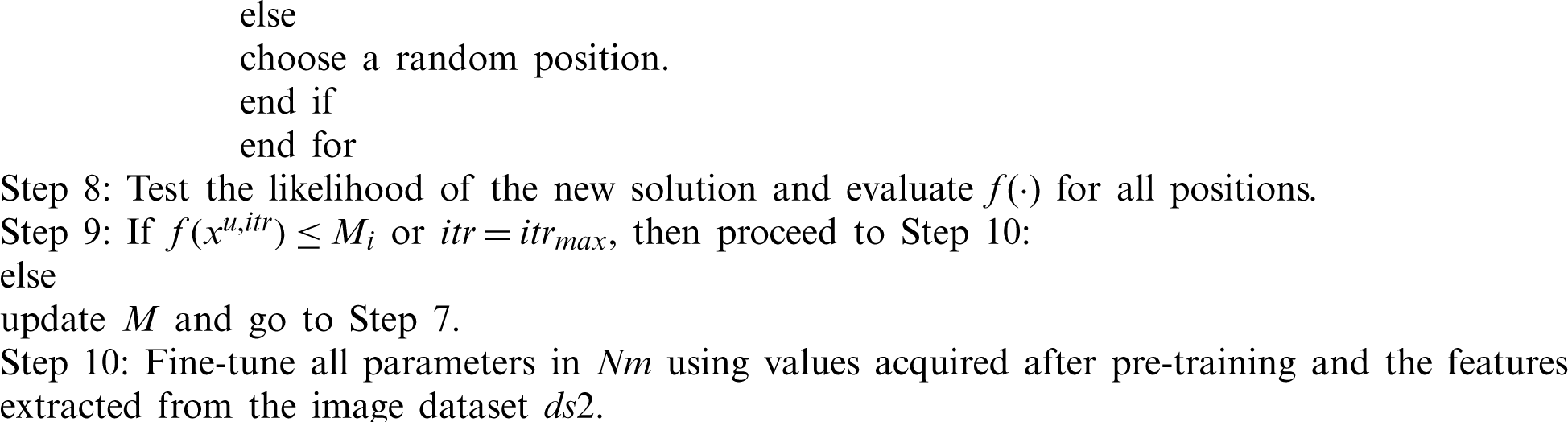
Individual steps in the proposed DNN-CSA module are provided in Algorithm 1. This approach was developed to maximize classification accuracy by reducing the error rate.
An open-source database of rice plant leaves is not presently available. As such, we collected a total of 120 photographs of normal and diseased rice plant leaves using a NIKON D90 digital SLR camera with image dimensions of
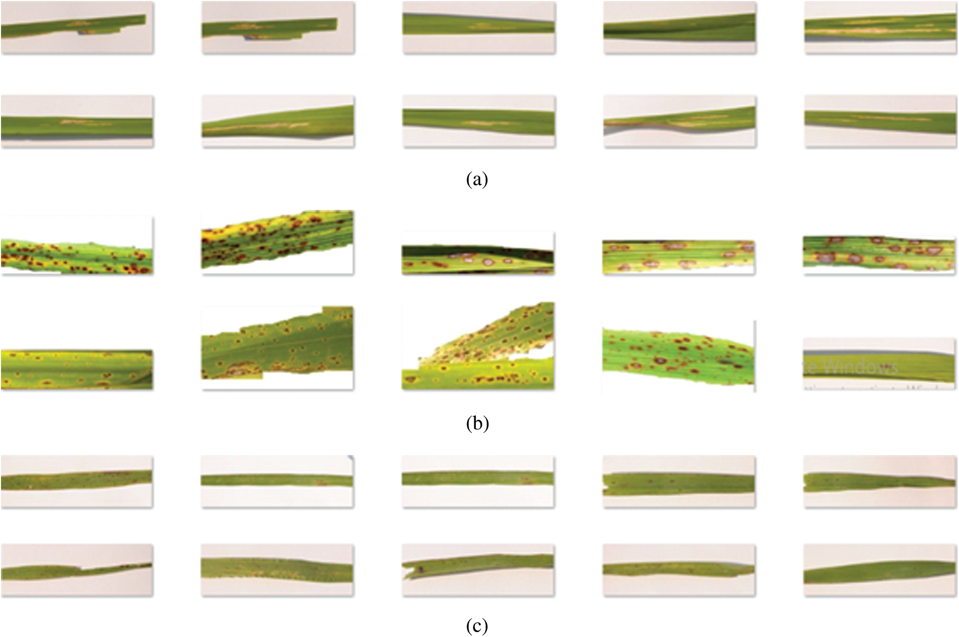
Figure 2: Sample images (a) bacterial leaf blight (b) brown spot (c) leaf smut
Examples of initial RGB images and segmented diseased regions are provided in Figs. 3a and 3b, respectively.
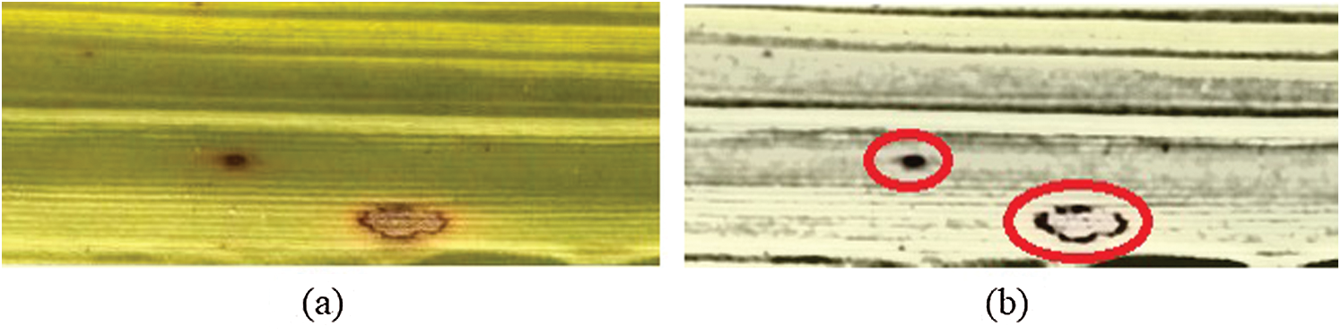
Figure 3: (a) Input image (b) disease segmented image
Rice disease classification results produced by the proposed DNN-CSA module were compared with those of an SVM algorithm during the training and testing phases. Two different multiple cross-fold validations (accuracy and precision) were used as recall metrics. Accuracy is defined as the number of correctly classified samples divided by the total number of samples:
Precision is defined as the ratio of correctly identified positive cases to all predicted positive cases:
Recall compares correctly identified positive cases to the actual number of positive cases:
In these expressions, TP denotes true positives, TN is true negatives, FP is false positives, and FN is false negatives.
The results shown in Tab. 1 and Figs. 4–6 demonstrate that the proposed DNN-CSA model offers superior classification performance, compared to an SVM algorithm, for the considered conditions. While the SVM performed well during the training phase, its classification accuracy was quite poor in the testing phase.
Table 1: Performance analysis of proposed method DNN-CS with state of art methods
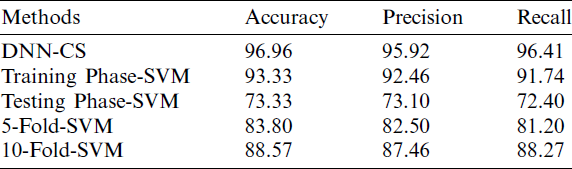
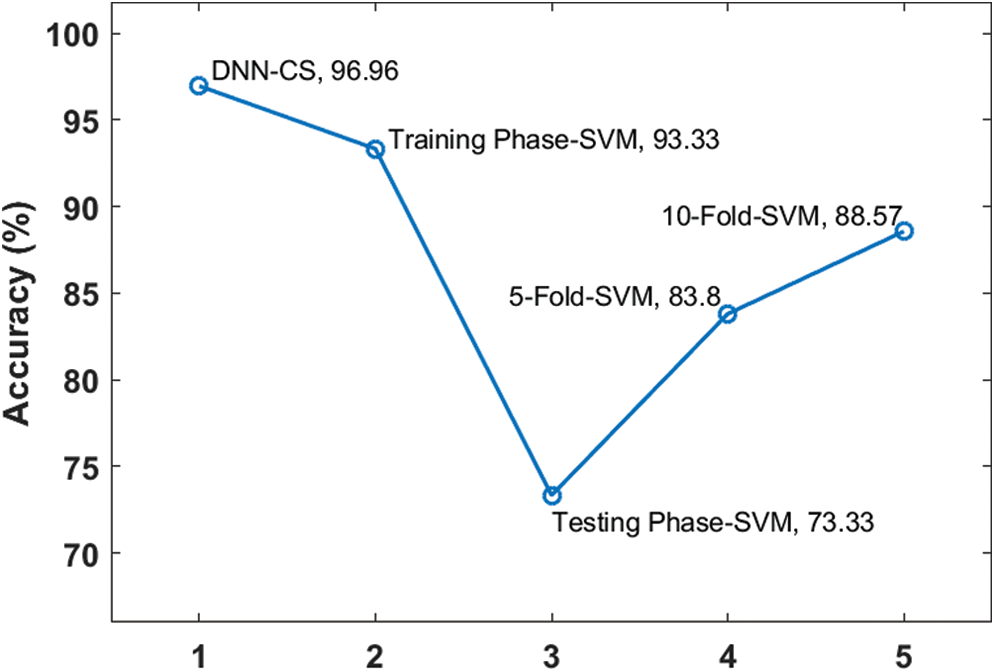
Figure 4: Accuracy analysis of proposed DNN-CS model
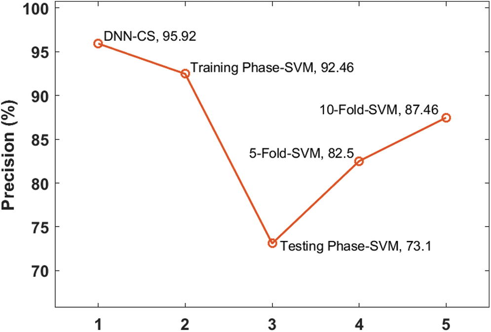
Figure 5: Precision analysis of proposed DNN-CS model

Figure 6: Recall analysis of proposed DNN-CS model
In fact, SVM accuracy remained inferior to that of the proposed model, even after applying cross-fold validation. The accuracy, precision, and recall values produced by the proposed algorithm were respectively 9.5%, 9.7%, and 9.2% higher than those of the 10-fold SVM.
This study addressed a lack of embedded computer vision techniques suitable for agricultural applications by proposing a novelDNN classification model for the identification of paddy leaf diseases in image data. Classification errors were minimized by optimizing weights and biases in the DNN model using the CSA, which was performed during both the standard pre-training and fine-tuning processes to establish a novel DNN-CSA architecture. This approach facilitates the use of simplistic statistical learning techniques together with a decreased computational workload to ensure both high efficiency and high classification accuracy. The performance of the proposed DNN-CSA for the identification of paddy leaf diseases was compared experimentally with that of an SVM algorithm under multiple cross-fold validation. In the experiments, the DNN-CSA achieved an accuracy of 96.96%, a precision of 95.92%, and a recall of 96.41%, each of which were more than 9% higher than that of a 10-fold validated SVM classifier. These results suggest the DNN-CSA could be applied in the future to assisting farmers in the detection and diagnosis of plant diseases in real time, using images collected in the field and loaded onto a remote device.
Funding Statement: The authors have received no specific funding for this research.
Conflicts of Interest: The authors declare that they have no conflicts of interest to report regarding the present study.
1. X. E. Pantazi, D. Moshou and A. A. Tamouridou. (2019). “Automated leaf disease detection in different crop species through image features analysis and one class classifiers,” Computers and Electronics in Agriculture, vol. 156, no. 1, pp. 96–104. [Google Scholar]
2. D. Y. Kim, A. Kadam, S. Shinde, R. G. Saratale, J. Patra et al. (2018). , “Recent developments in nanotechnology transforming the agricultural sector: A transition replete with opportunities,” Journal of the Science of Food and Agriculture, vol. 98, no. 3, pp. 849–864. [Google Scholar]
3. A. K. Singh, B. Ganapathysubramanian, S. Sarkar and A. Singh. (2018). “Deep learning for plant stress phenotyping: Trends and future perspectives,” Trends in Plant Science, vol. 23, no. 10, pp. 883–8898. [Google Scholar]
4. B. H. Prajapati, J. P. Shah and V. K. Dabhi. (2017). “Detection and classification of rice plant diseases,” Intelligent Decision Technologies, vol. 3, no. 3, pp. 357–373. [Google Scholar]
5. J. G. Barbedo, L. V. Arnal and T. T. S. Koenigkan. (2016). “Identifying multiple plant diseases using digital image processing,” Biosystem Engineering, vol. 147, no. 660, pp. 104–116. [Google Scholar]
6. S. Sladojevic, M. Arsenovic, A. Anderla, D. Culibrk and D. Stefanovic. (2016). “Deep neural networks based recognition of plant diseases by leaf image classification,” Computational Intelligence and Neuroscience, vol. 2016, no. 6, pp. 1–11. [Google Scholar]
7. P. Mohanty, D. P. Sharada and M. S. Hughes. (2016). “Using deep learning for image-based plant disease detection,” Frontiers in Plant Science, vol. 7, no. 9, pp. 1–10. [Google Scholar]
8. A. K. Mahlein. (2016). “Plant disease detection by imaging sensors– parallels and specific demands for precision agriculture and plant phenotyping,” Plant Disease, vol. 100, no. 2, pp. 241–251. [Google Scholar]
9. F. T. Pinki, N. Khatun and S. M. M. Islam. (2017). “Content based paddy leaf disease recognition and remedy prediction using support vector machine,” in Proc. 20th Int. Conf. on Computer and Information Technology, Dhaka, Bangladesh, pp. 1–5. [Google Scholar]
10. Y. Lu, S. Yi, N. Zeng, Y. Liu and Y. Zhang. (2017). “Identification of rice diseases using deep convolutional neural networks,” Neuro Computing, vol. 267, no. 12, pp. 378–384. [Google Scholar]
11. G. Dhingra, V. Kumar and H. D. Joshi. (2019). “A novel computer vision based neutrosophic approach for leaf disease identification and classification,” Measurement, vol. 135, no. 3, pp. 782–794. [Google Scholar]
12. A. D. Nidhis, C. N. V. Pardhu, K. C. Reddy and K. Deepa. (2019). “Cluster based paddy leaf disease detection, classification and diagnosis in crop health monitoring unit,” Computer Aided Intervention and Diagnostics in Clinical and Medical Images, vol. 31, pp. 281–291. [Google Scholar]
13. T. Islam, M. Sah, S. Baral and R. R. Choudhury. (2018). “A faster technique on rice disease detection using image processing of affected area in agro-field,” in Proc. Second Int. Conf. on Inventive Communication and Computational Technologies, Coimbatore, India, pp. 62–69. [Google Scholar]
14. T. Devi and P. N. Gayathri. (2019). “Image processing based rice plant leaves diseases in thanjavur tamilnadu,” Cluster Computing, vol. 6, pp. 1–14. [Google Scholar]
15. F. A. D. Santos, D. M. Freitas, G. G. D. Silva, H. Pistori and M. T. Folhes. (2017). “Weed detection in soybean crops using ConvNets,” Computers and Electronic Agriculture, vol. 143, no. 12, pp. 314–324. [Google Scholar]
16. A. Kaya, A. S. Keceli, C. Catal, H. Y. Yalic, H. Temucin et al. (2019). , “Analysis of transfer learning for deep neural network based plant classification models,” Computers and Electronics in Agriculture, vol. 158, no. 3, pp. 20–29. [Google Scholar]
17. S. Ramesh and D. Vydeki. (2020). “Recognition and classification of paddy leaf diseases using optimized deep neural network with java algorithm,” Information Processing in Agriculture, vol. 7, no. 2, pp. 249–260. [Google Scholar]
18. R. J. S. Raj, S. J. Shobana, I. V. Pustokhina, D. A. Pustokhin, D. Gupta et al. (2020). , “Optimal feature selection-based medical image classification using deep learning model in internet of medical things,” IEEE Access, vol. 8, pp. 58006–58017. [Google Scholar]
19. A. Askarzadeh. (2016). “A novel metaheuristic method for solving constrained engineering optimization problems: Crow search algorithm,” Computers & Structures, vol. 169, no. 6, pp. 1–12. [Google Scholar]
 | This work is licensed under a Creative Commons Attribution 4.0 International License, which permits unrestricted use, distribution, and reproduction in any medium, provided the original work is properly cited. |