DOI:10.32604/cmc.2021.015969
| Computers, Materials & Continua DOI:10.32604/cmc.2021.015969 | |
| Article |
Joint Frequency and DOA Estimation with Automatic Pairing Using the Rayleigh–Ritz Theorem
1College of Electrical and Information Engineering, Zhengzhou University of Light Industry, Zhengzhou, 450003, China
2Faculty of Engineering and Information Technology, University of Technology Sydney, Sydney, NSW, 2007, Australia
*Corresponding Author: Haiming Du. Email: duhaiming-007@zzuli.edu.cn
Received: 16 December 2020; Accepted: 23 January 2021
Abstract: This paper presents a novel scheme for joint frequency and direction of arrival (DOA) estimation, that pairs frequencies and DOAs automatically without additional computations. First, when the property of the Kronecker product is used in the received array signal of the multiple-delay output model, the frequency-angle steering vector can be reconstructed as the product of the frequency steering vector and the angle steering vector. The frequency of the incoming signal is then obtained by searching for the minimal eigenvalue among the smallest eigenvalues that depend on the frequency parameters but are irrelevant to the DOAs. Subsequently, the DOA related to the selected frequency is acquired through some operations on the minimal eigenvector according to the Rayleigh–Ritz theorem, which realizes the natural pairing of frequencies and DOAs. Furthermore, the proposed method can not only distinguish multiple sources, but also effectively deal with other arrays. The effectiveness and superiority of the proposed algorithm are further analyzed by simulations.
Keywords: Array signal processing; DOA estimation; automatic pairing; Rayleigh–Ritz theorem
Frequency estimation and DOA estimation for an antenna array are the basic but key problems in the area of array signal processing [1–3], e.g., in the applications of direction finding, radar, sonar, wireless communications, and especially location service [4,5] under the scenario of multiple incoming signals with different frequencies. The maximum likelihood (ML) method [6] is often applied but brings a great computational load. To reduce the computational effort required, the multiple signal classification (MUSIC) algorithm [7], some ESPRIT-based joint angle and frequency estimation methods [8,9] and the propagator method (PM) [10] have been proposed. However, the MUSIC method [7] requires spectral peak searching in both the frequency range and angle range, and this is still computationally expensive, particularly for 2-dimensional arrays. The PM [10] has low complexity, but its parameter estimation performance is poorer than that of the ESPRIT algorithm. Unfortunately, ESPRIT is only applicable to a uniform linear array. In [11], the iterative least-squares method was used for joint frequency and DOA estimation with L-shaped arrays, and many iterations were needed for convergence.
Using multiple-delay outputs, the authors in [12] proposed a joint angle and frequency estimation method based on ESPRIT; this approach outperforms the conventional ESPRIT algorithm, but it not only requires additional pairing operations [13] but is also only suitable for uniform linear arrays. In addition, the angle estimation procedure only utilizes part of the received signals. The ESES method proposed in a recent study [14] has the same procedure for estimating frequency as the method in [12], but unlike in [12], all of the received signals are used to estimate the angle in [14]; thus, the performance is better than the method developed in [12]. The ESES approach [14] can also be employed for other array structures. However, the ESES method in [14] carelessly neglects that the eigenvalues of two matrices from the different permutations of one matrix may not be in the same order, so the frequencies and angles obtained from the eigenvalues require some additional computations for pairing those parameters (as in [13]), and the process cannot always arrive at the correct pairings under some conditions.
To pair the frequency and angle estimations automatically and avoid potential pairing mistakes, relative to the multiple-delay output model used in [12,14], this paper is an improvement and presents a novel joint frequency and angle estimation algorithm without additional pairings owing to the Rayleigh–Ritz theorem [15, Section 4.2]. Frequencies can be calculated by a one-dimensional search, and angles can be obtained as closed-form solutions. Furthermore, the proposed algorithm can work with other arrays, such as nonuniform linear arrays. Hence, a unified framework for joint frequency and angle estimations is established by the proposed algorithm. In addition, the proposed method has better estimation performance than that of the ESES method in [14] and has acceptable computational complexity, which is confirmed by simulation results.
An outline of this paper is as follows. Section 2 describes the data model. Section 3 addresses the algorithmic issues encountered with some remarks. Section 4 shows the simulation results, which are followed by conclusions in Section 5.
Notations:  ,
,  , and
, and  denote the transpose, conjugate transpose and pseudoinverse operations, respectively; diag(v) stands for a diagonal matrix whose
  diagonal element is the
  entry in vector v; IM is an
  identity matrix;
  represents the Kronecker product;
  is the rank of the chosen matrix;
  returns the phase angle of the chosen element; and
  and
and  stand for the maximum and minimum arguments, respectively.
Consider an arbitrary array of M sensors on which K (assuming K is known in this study) incident waves impinge; if the sources are all narrow-band signals without the same center frequency, the signal received at the  antenna can be expressed as

where  are the frequency and narrow-band signal of the
  source, respectively.
  represents spatially and temporally additive Gaussian white noise with zero mean.
  is the time delay of the
  sensor; therefore, it depends on the structure of the array and the
  incoming angle of the received signal. Thus,
  of the uniform linear array can be denoted by

where d is the distance between the adjoining sensors, c is the velocity of light, and  is the incoming angle of the
  source. The output of the array is

The received signal of array antennas can be shown in matrix form as

where
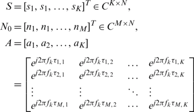
The angle steering vector is
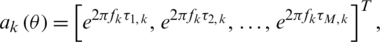
and the delayed signal for (1) with  can be written as
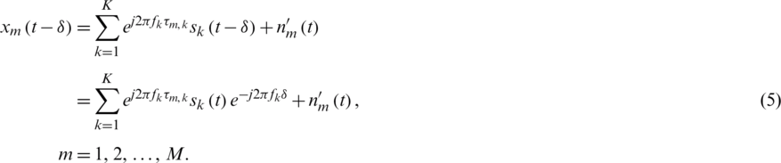
Afterwards, the delayed signal for (5) with  can be denoted as

where  ,
,  ,
,  .
.
Therefore, the delayed signal for (1) with  can be expressed as

where P is the number of delays.
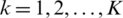
According to (4), (6) and (7), the multiple-delay output model [12,14] can be described as
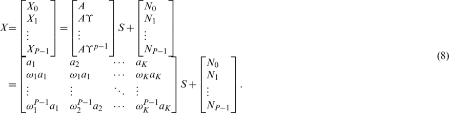
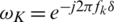
Define the frequency steering vector  ,
,  . Then, (8) can be reconstructed as

where  is the frequency-angle steering vector.
3 Joint Frequency and Angle Estimation
From (9), we know that the frequency fk and angle  can be estimated by attaining
  and ak from the received array signal. The covariance matrix of the received signal can be calculated via Rxx = XXH. Using the eigenvalue decomposition of Rxx, we can obtain En, which is the noise space spanned by the
  eigenvectors corresponding to the minimal
  eigenvalues of the covariance matrix Rxx. Hence, the frequency fk and angle
  can be obtained by the MUSIC algorithm [1,7] as
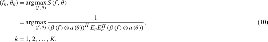
However, to obtain all source parameters  from (10), an exhaustive search in the two-dimensional space is generally required, thereby resulting in a heavy computational burden. Here, by the property of the Kronecker product, a novel implementation of the two-dimensional parameter estimation process without the exhaustive two-dimensional search is developed based on the Rayleigh–Ritz theorem [15, Section 4.5].
By the property of the Kronecker product, the frequency-angle steering vector can be reformulated in the following form

From (11), it is obvious that the frequency-angle steering vector is decomposed into the product of one matrix 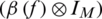 that is only related to the frequency steering vector and the other matrix
  that is only concerned with the angle steering vector; this product lays a foundation for estimating fk and
  separately and enables us to avoid a two-dimensional search.
Inserting (11) into (10), we can obtain

Define

where  is an
is an  Hermitian matrix dependent on f and independent of
  . Thus, (12) can be rewritten as
Since  is a Hermitian matrix, the Rayleigh quotient of
  is a scalar that can be defined as

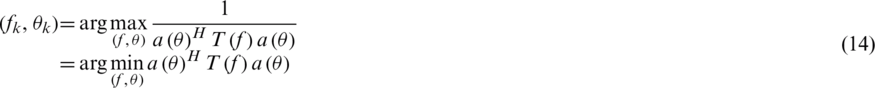
Notice that  and
and 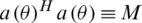 ; thus, (14) can be converted into a Rayleigh quotient problem:
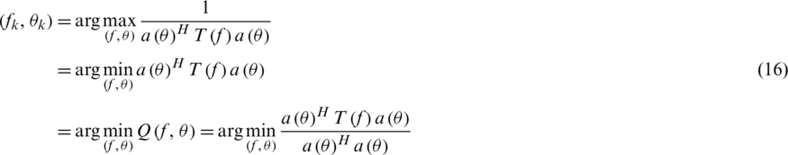
If f does not correspond to one of the true values, and if

then,  is invertible, and its eigenvalues are all greater than zero. According to the Rayleigh–Ritz theorem in [15], the minimum value of the objective in (16) is the minimum eigenvalue of
  , and in this case,
  should be proportional to the minimum eigenvector of
  ; thus, the frequency fk satisfies

and  has the following relationship with
  :
:

where  is the minimal eigenvalue of the matrix
  ,
,  is the eigenvector corresponding to the minimal eigenvalue of the matrix
  , and h is a constant. There are many fast algorithms, such as [16], for finding the minimal eigenvalue and eigenvector of a Hermitian matrix.
To solve for  from (19), let
  denote the
  phase angle of the
  element of the eigenvector
  , that is,
  , where
  is the
  element of
  . Then, it follows that

in which 
For an unambiguous uniform linear array, the interspacing between two adjacent elements d is not greater than  (
( is the wavelength of the signal), so
  and kq = 0. Afterwards, recall the fk obtained by (18), and the accurate value of
  can be estimated by solving the equation set of (20) using the least-squares method.
It should be pointed out that  is obtained by inserting fk into (19) and solving the equation set of (20); thus, it is inferred that fk and
  are paired naturally.
The proposed method can also address the case in which multiple signals have the same frequency but different DOAs by distinguishing the number of minimal eigenvalues with respect to fk in (18) and their corresponding eigenvectors in (19).
Because the frequency is obtained via an eigenvalue and the angle is obtained via an eigenvector, this method is named the EVEV algorithm.
It is worth noting that to obtain the frequency fk from (18), a one-dimensional search in the frequency space is required. If the true frequency lies in a set with few values, there is little computational expense. In contrast, if the estimated frequency depends on a wide range of frequencies, this may lead to a great computational load. To pursue a more convenient implementation of joint frequency and angle estimation than the EVEV algorithm, the DOA  can be found from (20) subsequent to the frequency fk estimated by the ESPRIT algorithm, as in [12,14].
By the eigenvalue decomposition of Rxx, the signal subspace Es is spanned by the K eigenvectors corresponding to the first K maximal eigenvalues. Then, we divide Es into E1 (the first  rows of Es) and E2 (the last
  rows of Es). Define

Then we can obtain the eigenvalues 
 of the matrix
  . Finally, the frequency fk is estimated by (see [12,14] for more information)

Subsequently, based on the Rayleigh–Ritz theorem,  is constructed with (13), and then the DOA is obtained by substituting the fk obtained from (22) into (20), as in the previous subsection. This method, which is named the ESEV algorithm, is a combination of the ESES method in [14] and the EVEV method proposed in this study, and it provides joint frequency and angle estimations in closed-form solutions.
In this section, we analyze the computational complexities of the EVEV and ESEV algorithms and compare them with that of the ESES method [14]. For the EVEV algorithm, obtaining the covariance matrix estimation Rxx requires  flops, obtaining En through the eigendecomposition of Rxx costs
  flops, and the estimation of
  and obtaining the minimal eigenvalue of
  and its eigenvector via several iterative methods requires
  flops. Thus, the total computational complexity of the EVEV algorithm is
  flops, where r is the number of search grids within the search frequency region. To pair the frequency and DOA, the ESES method needs
 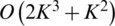 flops. Hence, the ESES algorithm requi- res
  flops in total. Therefore, the proposed ESEV algorithm needs
  flops.
It can be concluded that the EVEV method has the largest computational complexity among these three methods if the number of search grids r is large. Furthermore, both the ESEV and ESES methods provide frequency and DOA estimations in closed-form solutions, as mentioned previously, so their computational complexities with respect to r are irrelevant. In addition, the ESEV method has almost the same computational complexity as that of the ESES method.
From these aforementioned derivations, some remarks can be made:
Remark 1: From (17), the number of resolvable sources satisfies  ; however, (18) indicates that K must not be greater than the dimension of the matrix
  , that is,
  . In general, the number of delays satisfies
  , so the maximum number of resolvable sources satisfies
  for the EVEV method. The ESES method only estimates the frequency and DOA if
  ; therefore, the maximum numbers of resolvable sources for the ESES and ESEV methods also satisfy
  . The abilities of these three methods to resolve multiple sources, based on the multiple-delay output model, exceed those of conventional algorithms [6–11], which can resolve at most
  sources.
Remark 2: Both the EVEV algorithm and ESEV algorithm can achieve the automatic pairing of the estimation parameters. The angle  is obtained by inserting fk into (19); thus, the frequency fk and direction of arrival
  can be paired naturally with both the EVEV and ESEV methods.
Remark 3: Both the EVEV algorithm and ESEV algorithm can be applied to arbitrary arrays. Obtaining the frequency from (18) or (22) is irrelevant to the array geometry, and angle estimation can be realized from (20) based on prior information about the array structure. Therefore, the two proposed methods have no dependencies on the array configurations and can be used with any array, for example, a nonuniform linear array.
Remark 4: From the delay segment  in (5), it is easy to see that the delay time must satisfy
  to avoid ambiguity in the estimation of the frequency fk; this is a milder requirement for
  than
than  in [12].
Remark 5: The EVEV, ESEV and ESES methods can all deal with the case in which two or more signals have the same frequency but are from different incoming DOAs. In contrast, none of these methods can work effectively in a coherent source environment.
The performances of the proposed methods are evaluated with some Monte Carlo simulations. In the following experiments, assume that M is the number of antennas, P is the number of delays, L is the number of snapshots, and K is the number of sources. The distance between two adjacent elements in the uniform linear array is half of the wavelength of the maximum estimated frequency, and the other parameters are M = 10, P = 3, L = 200, signal-to-noise ratio SNR = 20 dB, sampling frequency fs = 2000000 HZ and delay time  . The following results are evaluated by the estimated root mean square errors (RMSEs) obtained from the average results of 2000 Monte Carlo simulations. Frequency RMSE stands for the RMSE of the estimated frequencies, and DOARMSE stands for the RMSE of the estimated DOAs. If there is no additional instruction, these parameters all hold in the simulations. In addition, we compare EVEV and ESEV with ESES [14], which has the same data model as the one in this study.
Simulation 1. The performance of ESES is investigated. Tab. 1 indicates the results of the ESES, EVEV and ESEV methods when the angles are  ,
,  and
and  , and their carrier frequencies are 200000, 400000 and 800000 HZ, respectively. From Tab. 1, it is easy to see that the ESES method has estimation ambiguity with respect to the angles, and there are two DOAs for 200000HZ and three DOAs each for 400000 and 800000 HZ. For example, there are three DOAs
  ,
,  and
and  corresponding to the frequency 400000 HZ, so additional computations [13] are needed for determining the true frequency and angle pair. In contrast, neither the EVEV nor the ESEV method requires additional pairing computations.
Table 1: DOA estimation of ESES, EVEV and ESEV

Simulation 2. The performances of the proposed algorithms (EVEV and ESEV) are examined. Figs. 1 and 2 display the outcomes of the EVEV method and ESEV method when the angles of the 10 incoming signals are  ,
,  , and
, and  with the same frequency of 200000 HZ;
  ,
,  ,
,  , and
, and  with the same frequency of 400000 HZ; and
  ,
,  and
and  with the same frequency of 800000 HZ. From Figs. 1 and 2, we find that the EVEV and ESEV methods can not only obtain the frequency and angle estimations correctly without pairing ambiguity but can also resolve
  sources. However, the ESES method cannot handle this case.
Figure 1: Frequency and DOA estimation performance of EVEV
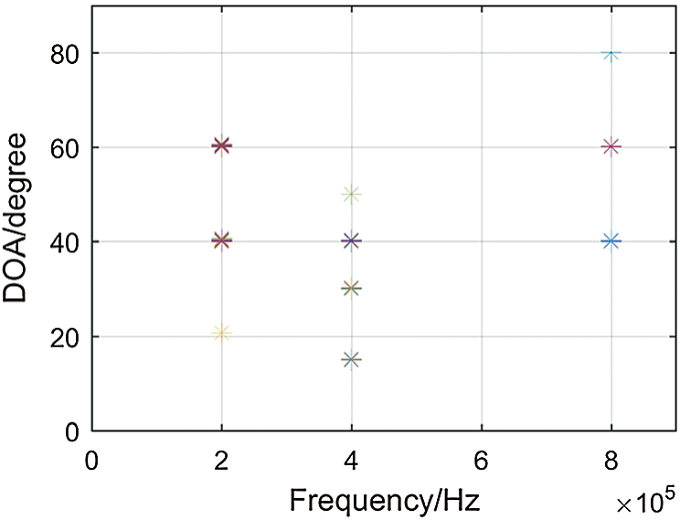
Figure 2: Frequency and DOA estimation performance of ESEV
Simulation 3. The performances of ESES, ESEV and EVEV under different SNRs and different numbers of snapshots are studied in this simulation. All the simulation conditions are the same as those in Simulation 1 except for the following descriptions. The number of snapshots for each experiment is set to 200, and the SNR is changed from 0 to 30 dB for the three sources. Figs. 3 and 4 show the simulation results of the frequency and DOA parameters when the SNR changes, respectively. Then, the SNR is fixed to 20 dB, and the number of snapshots is varied from 100 to 800. In this case, the simulation results of the frequency and DOA parameters are illustrated in Figs. 5 and 6, respectively.
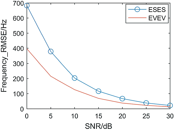
Figure 3: The RMSEs of the frequency estimations vs. the SNR
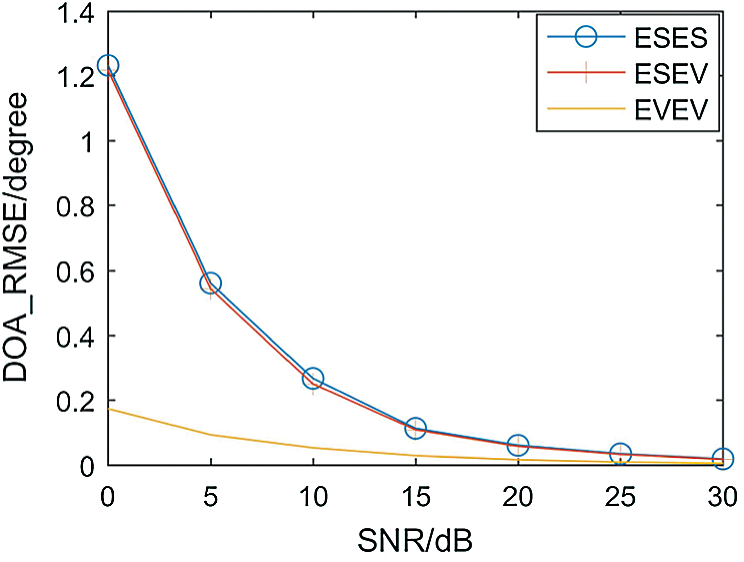
Figure 4: The RMSEs of the DOA estimations vs. the SNR
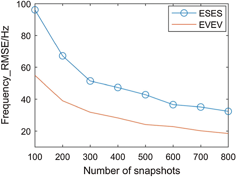
Figure 5: The RMSEs of the frequency estimations vs. the number of snapshots
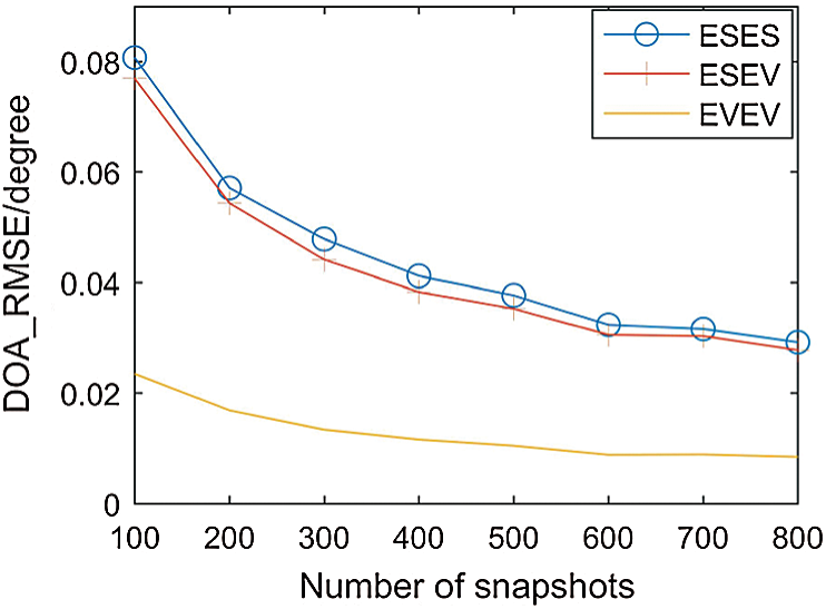
Figure 6: The RMSEs of the DOA estimations vs. the number of snapshots
From Figs. 3–6, it can be observed that all three methods are effective for joint frequency and angle estimation. In addition, when the SNR or the number of snapshots increases, the RMSEs of both the frequency and angle estimations decrease. Figs. 3 and 5 illustrate that the frequency estimation performance of the EVEV method is better than that of the ESES method. Additionally, it can be seen from Figs. 4 and 6 that the angle estimation performance of the ESEV method is slightly better than that of the ESES method. In addition, note that the ESEV method has the same frequency estimation result as that of the ESES method and the same angle estimation result as that of the EVEV method. Therefore, from Figs. 4 and 6, it is inferred that the angle estimation performance of the EVEV method is better than that of the ESES method.
Simulation 4. The computational complexities of these three methods are compared in this subsection. Suppose M = 10, P = 3 and K = 3, as in Simulations 1 and 3. For simplicity of comparison with other methods, the number of search grids r = 20 for the EVEV method. When the number of snapshots is varied from L = 100 to L = 2000, Fig. 7 shows the computational complexities of the three methods. The EVEV algorithm has the largest computational complexity under this condition. In fact, the computational burden of EVEV becomes heavier as r increases. It can also be seen from Fig. 7 that the ESEV algorithm has almost the same computational complexity as that of the ESES method. In summary, these results coincide with the aforementioned theoretical analysis.
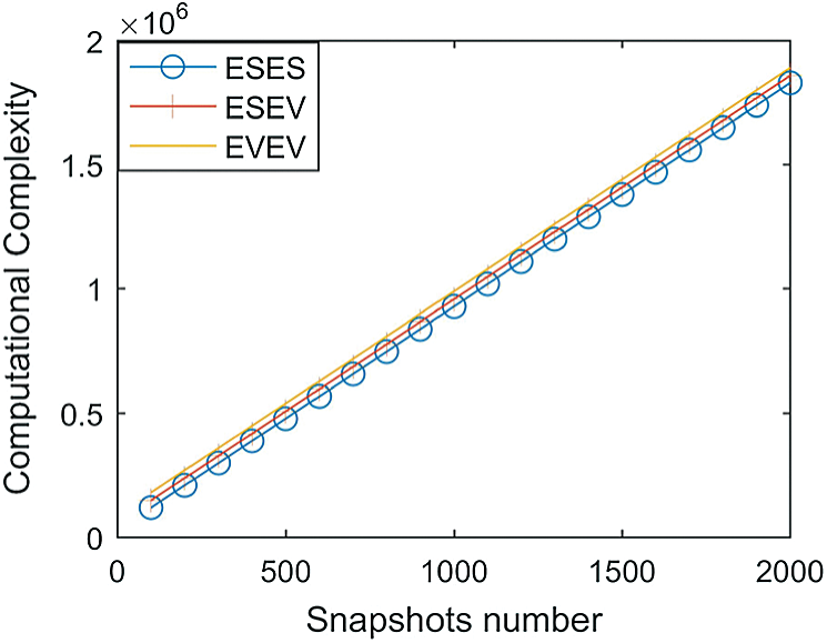
Figure 7: Computational complexity of ESES, ESEV and EVEV
Simulation 5. The effectiveness of ESES, ESEV and EVEV in handling a nonuniform linear array is studied. Assume that eight sensors are located at positions  and normalized by half of the wavelength. The three sources are from
  ,
,  and
and  with different frequencies for different methods. From Fig. 8, it is verified that all three methods can work well with the nonuniform linear array.
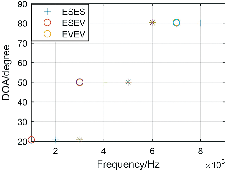
Figure 8: Frequency and DOA estimation for a nonuniform linear array
This paper has considered the problem of joint frequency and DOA estimation in array signal processing. By applying the Rayleigh–Ritz theorem to the multiple-delay output model, the proposed methods can achieve automatically paired frequency and DOA estimations without an exhaustive two-dimensional search. The investigations, which were demonstrated in theory and through the use of extensive simulations, have shown that the proposed methods have better estimation performances than those of the ESES and ESEV methods, making a good compromise between estimation accuracy and computational complexity compared with EVEV and ESES. Furthermore, the proposed two methods can always resolve no fewer sources than can ESES. In addition, these methods can also be used for other arrays, including but not limited to nonuniform linear arrays. Future research might be expected to extend the applications of these methods to situations in the presence of multiple coherent sources, array gain-phase errors or mutual coupling effects among the examined sensors.
Acknowledgement: The authors acknowledge the help of their colleagues and families.
Funding Statement: This work was supported by the colleges and universities of the Key Projects Scientific Research Plan of Henan Province (19B413005). The authors are grateful for their support.
Conflicts of Interest: The authors declare that they have no conflicts of interest to report regarding the present study.
1. R. Schmidt. (1986). “Multiple emitter location and signal parameter estimation,” IEEE Transactions on Antennas and Propagation, vol. 34, no. 3, pp. 276–280. [Google Scholar]
2. V. V. Reddy, B. P. Ng and A. W. H. Khong. (2013). “Insights into MUSIC-like algorithm,” IEEE Transactions on Signal Processing, vol. 61, no. 10, pp. 2551–2556. [Google Scholar]
3. Y. J. Sun, Y. Q. Yuan, Q. Wang, L. H. Wang, E. L. Li et al. (2019). , “Research on the signal reconstruction of the phased array structural health monitoring based using the basis pursuit algorithm,” Computers Materials & Continua, vol. 58, no. 2, pp. 409–420. [Google Scholar]
4. J. Wang, X. H. Qiu and Y. F. Tu. (2019). “An improved MDS-MAP localization algorithm based on weighted clustering and heuristic merging for anisotropic wireless networks with energy holes,” Computers Materials & Continua, vol. 60, no. 1, pp. 227–244. [Google Scholar]
5. W. Y. Liu, X. Y. Luo, Y. M. Liu, J. Q. Liu, M. H. Liu et al. (2018). , “Localization algorithm of indoor Wi-Fi access points based on signal strength relative relationship and region division,” Computers Materials & Continua, vol. 55, no. 1, pp. 71–93. [Google Scholar]
6. M. Djeddou, A. Belouchrani and S. Aouada. (2005). “Maximum likelihood angle-frequency estimation in partially known correlated noise for low-elevation targets,” IEEE Transactions on Signal Processing, vol. 53, no. 8, pp. 3057–3064. [Google Scholar]
7. J. D. Lin, W. H. Fang, Y. Y. Wang and J. T. Chen. (2006). “FSF MUSIC for joint DOA and frequency estimation and its performance analysis,” IEEE Transactions on Signal Processing, vol. 54, no. 12, pp. 4529–4542. [Google Scholar]
8. A. N. Lemma, A. J. Van der Veen and E. Deprettere. (1998). “Joint angle-frequency estimation using multi-resolution ESPRIT,” in Proc. IEEE Int. Conf. on Acoustics, Speech and Signal Processing, Seattle, Wash, USA, pp. 1957–1960. [Google Scholar]
9. A. N. Lemma, A. J. Van Der Veen and E. F. Deprettere. (2003). “Analysis of joint angle-frequency estimation using ESPRIT,” IEEE Transactions on Signal Processing, vol. 51, no. 5, pp. 1264–1283. [Google Scholar]
10. L. L. Xu, X. F. Zhang and Z. Z. Xu. (2010). “Improved joint direction of arrival and frequency estimation using propagator method,” in Proc. IEEE Int. Conf. on Information Science and Engineering, Hangzhou, China, pp. 2139–2142. [Google Scholar]
11. L. Y. Xu, X. F. Zhang, Z. Z. Xu and M. Yu. (2012). “Joint 2D-DOA and frequency estimation for L-shaped array using iterative least squares method,” International Journal of Antennas and Propagation, vol. 2012, Article ID 983092, 9 pages. [Google Scholar]
12. X. D. Wang. (2010). “Joint angle and frequency estimation using multiple-delay output based on ESPRIT,” EURASIP Journal on Advances in Signal Processing, vol. 2010, Article ID 358659, 6 pages. [Google Scholar]
13. D. F. Chen, B. X. Chen and G. D. Qin. (2008). “Angle estimation using ESPRIT in MIMO radar,” Electronics Letters, vol. 44, no. 12, pp. 770–771. [Google Scholar]
14. X. D. Wang, X. F. Zhang, J. F. Li and J. C. Bai. (2012). “Improved esprit method for joint direction-of-arrival and frequency estimation using multiple-delay output,” International Journal of Antennas and Propagation, vol. 2012, Article ID 309269, 10 pages. [Google Scholar]
15. R. A. Horn, C. R. Johnson and H. Matrices. (2012). “Symmetric matrices, and congruences,” in Matrix Analysis, 2 ed., vol. 9. Cambridge: Cambridge University Press, pp. 225–312. [Google Scholar]
16. X. Yang, T. K. Sarkar and E. Arvas. (1989). “A survey of conjugate gradient algorithms for solution of extreme eigen-problems of a symmetric matrix,” IEEE Transactions Acoustics, Speech, Signal Processing, vol. 37, no. 10, pp. 1550–1556. [Google Scholar]
 | This work is licensed under a Creative Commons Attribution 4.0 International License, which permits unrestricted use, distribution, and reproduction in any medium, provided the original work is properly cited. |