DOI:10.32604/cmc.2021.015495
| Computers, Materials & Continua DOI:10.32604/cmc.2021.015495 | |
| Article |
Parallel Optimization of Program Instructions Using Genetic Algorithms
Department of Electronics, Communications and Computers, University of Pitesti, Pitesti, 110040, Romania
*Corresponding Author: Petre Anghelescu. Email: petre.anghelescu@upit.ro
Received: 24 November 2020; Accepted: 12 January 2021
Abstract: This paper describes an efficient solution to parallelize software program instructions, regardless of the programming language in which they are written. We solve the problem of the optimal distribution of a set of instructions on available processors. We propose a genetic algorithm to parallelize computations, using evolution to search the solution space. The stages of our proposed genetic algorithm are: The choice of the initial population and its representation in chromosomes, the crossover, and the mutation operations customized to the problem being dealt with. In this paper, genetic algorithms are applied to the entire search space of the parallelization of the program instructions problem. This problem is NP-complete, so there are no polynomial algorithms that can scan the solution space and solve the problem. The genetic algorithm-based method is general and it is simple and efficient to implement because it can be scaled to a larger or smaller number of instructions that must be parallelized. The parallelization technique proposed in this paper was developed in the C# programming language, and our results confirm the effectiveness of our parallelization method. Experimental results obtained and presented for different working scenarios confirm the theoretical results, and they provide insight on how to improve the exploration of a search space that is too large to be searched exhaustively.
Keywords: Parallel instruction execution; parallel algorithms; genetic algorithms; parallel genetic algorithms; artificial intelligence techniques; evolutionary strategies
The importance of parallel instruction execution for our digital society is undeniable, and the development of fast processing algorithms raises interesting research questions in a wide range of fields: Aerospace technology, banking systems, CAD/CAM technologies, and IoT. Modern society depends on the parallel processing capabilities of electronic devices, and we would not be able to maintain our current operations without different optimization techniques. However, there is currently no polynomial algorithm capable of parallelizing software instructions.
Optimizing parallel computing algorithms is an open research field. Research methods generally involve finding a series of suboptimal solutions that asymptotically tend to the optimal solution. For some poorly optimized problems, probabilistic algorithms can be used to improve efficiency. They usually do not guarantee the best solution, but there is a chance that, through random selection, they will approach the proposed goal. In addition, analytical models cannot be applied to such problems either, because the problem of optimal distribution in multiprocessor systems is not a typical problem of the extremum. It has been shown that this type of problem is NP-complete (there are no polynomial algorithms capable of providing solutions) [1].
Running parallel instructions on multiple processors becomes more difficult in the case of additional communication constraints between processors. For example, there are dependencies between the instructions executed in parallel on different processors, dependencies between the instructions on the same processor, and dependencies between instructions on different processors, that are not executed in parallel. Optimization for parallel computation is generally based on broad and poorly structured search areas. For this reason, heuristic techniques are much more appropriate. Artificial intelligence methods provide effective solutions, and genetic algorithms, a type of evolutionary strategies, are perfectly suitable for complex optimization. Moreover, if a task is properly encoded, in some cases, it is possible to obtain better results than analytical approaches.
This paper is structured in five sections as follows. Section 2 provides a brief review of the parallelization of program instructions and genetic algorithms used for exploring large search spaces. Section 3 presents our method for the parallelization of software program instructions and our implementation of the genetic algorithm-based solution. Section 4 contains experimental results, with a focus on the functional performance in terms of processing speed and quality of the obtained results. Finally, Section 5 discusses our findings and sets some goals for future research directions.
2 Basic Concepts on Parallelization of Program Instructions and Genetic Algorithms
In this section, we briefly present the literature on the parallelization of program instructions and existing genetic algorithms-based models.
2.1 Parallelization of Program Instructions
The parallelization of program instructions or instruction scheduling is performed with a set of program instructions and a number of functional units. As reported by [2] the task involves selecting, from the large number of possible arrangements of concurrent instructions, one combination that decreases both the program space and the runtime. Scheduling methods include local scheduling and global scheduling. Existing instruction scheduling methods can be classified into linear methods [3], backtracking algorithms [4], constraint programming [5], machine learning based on reinforcement and rule-based learning [6–13], simulated annealing [14,15] and list scheduling [16,17]. List scheduling uses a directed acyclic graph and a heuristic algorithm that ends when all program instructions have been scheduled on the available functional units. List scheduling depends on the value of the heuristic used to select the best possible arrangement of instructions in the frontier list. In [18], a group of transformations were applied to the data dependency graph to solve the local instruction scheduling problem.
It has been proven that there are no polynomial algorithms that can scan the solution space and solve the instruction scheduling problem [1]. An alternative is the use of list and genetic algorithms to search through the problem space and find suitable solutions. In [19], a solution based on the injection of randomness in the instruction scheduling list was presented. The solution space was explored by randomly choosing instructions from the frontier list, instead of choosing the first one.
Research has been conducted on the different heuristics that can be applied for different computer architectures. The aim of the artificial intelligence-based strategies, including genetic algorithms, is to move away from investigating regions of the search space that do not produce significant results. In [20], the authors used a perceptron variant in which the weights are adjusted using heuristics. This patent did not give detailed experimental results, but the proposed variant is time-consuming. A group of researchers, in [21,22], proposed the use of genetic algorithms to scan the solution space and to adjust the heuristics values depending on various hardware targets in a greedy scheduler.
An interesting approach was presented in [23] in which the instruction scheduling, for optimizing embedded software performance includes building a data dependency graph for each basic block in an assembly program. A genetic technique was used to find the correct order of instructions with the highest performance, minimum execution time, for different kinds of processor architectures.
In [24,25], meta-heuristic techniques were proposed to solve the task scheduling problem using heterogenous computing systems. The authors proved that task scheduling is NP-complete for certain computer architectures and a genetic-based algorithm with a multi-objective fitness function reduces the runtime, increases the scheduling efficiency, and can reach a relatively optimal solution. Another interesting question, presented in [26], was how to design a general genetic algorithm that can adapt to various models of scheduling problems. The results of this paper showed that, for non-identical parallel machine scheduling, there is no ideal genetic algorithm, and their numerical example shows a promising execution time.
In [27], a genetic algorithm evolved a cellular automaton to perform instruction scheduling. This paper suggested two phases: In the first phase, the learning phase, the genetic algorithm is used to discover the suitable cellular automata rules for solving the instruction scheduling problem; in the second phase, the operation phase, the cellular automata operate as a parallel scheduler.
Taking previous research into consideration, we investigated instruction scheduling techniques, and we designed and developed a general genetic algorithm applicable to different parallelization methods and functional units. By investigating the way solutions are found, we improved our understanding of instruction scheduling and proposed optimized arrangements of concurrent instructions for different implementations.
2.2 Basic Concepts of the Genetic Algorithms
The beginnings of genetic algorithms are rooted in the 1950s, when several biologists suggested using computers to simulate biological systems. Later it was found that genetic algorithms were powerful computing tools for optimization problems. Therefore, models for finding optima in complex problems were established using the basic principles of genetics [28,29]. The core of genetic algorithms is to reproduce the mechanisms that govern the evolution of species in nature.
There are several forms for a genetic algorithm [30], but the commonest form is the following:

The algorithm above requires some discussion. First, the initial population is generated by randomly creating a fixed number of chromosomes, with each chromosome being a valid solution to the problem at hand. An evaluation function is then applied to each individual in the population [31]. The evaluation function is chosen that reflects the proximity or the distance of an individual from the optimal solution to the problem. A good genetic algorithm depends on the proper choice of this function. The selection of individuals to be crossed can be done in several ways. The commonly used technique is based on the Russian roulette, which has a number of slots equal to the number of individuals representing the population. The size of each slot is proportional to the value of the evaluation function applied to the individual. In other words, if an individual is closer to the optimal solution, it is more likely to be selected for the crossover. The selection procedure maintains superior solutions and removes inferior ones based on the fitness value at each iteration [32]. Of course, selection alone cannot find new points in the search space, so technically it cannot insert new individuals in population. For this reason, a crossover probability can be used, to select a part of the population for crossover. Along with the population size, this probability is one of the genetic algorithm’s parameters and generally has values above 30%. Another parameter is the mutation probability, based on which individuals are selected. Subsequently, the mutation operator is applied to them. In this way, new, and possibly better, individuals are obtained. The mutation probability generally has low values, below 5%. Finally, the  value is the parameter that represents the maximum number of generations for which the algorithm is run.
In this section, we present our method for the parallelization of program instructions. First, we describe the parallelization steps and the construction of the general data dependence graph using an example. Second, we present our genetic algorithm in detail. Third, we illustrate our algorithm with a general diagram and describe our implementation.
3.1 Problem Description and Representation
A software program consists of a set of instructions, each of them with associated latencies. Parallelization is possible when there are multiple processors that can execute the instructions. The goal is to rearrange the program’s instructions so that the number of the unparalleled instructions and the makespan (task execution time) are minimized. In order to describe the problem, let a program consist of several instructions that we number in the order of their appearance:
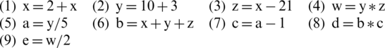
Using two processors, to parallelize, we can distribute these instructions as presented in Tab. 1.
Table 1: A possible example of instruction scheduling on two processors
In this example, we could parallelize instructions (1) and (2) because there are no data dependences between them, as well as (3) and (5), (6) and (7), and (4) and (8) for the same reason. However, we cannot parallelize (3) and (4) because to calculate w, in (4), z is required, but z is modified in (3), so there is a data dependence between instructions (3) and (4). Also, instruction (3) depends on (1), because (3) needs x, which is modified in (1). Moreover, instructions (1) and (3) must appear in this order. Instructions (4) and (5) depend on (2) and (4) depends on (2) and (3), so (4) must appear after (2) and (3).
We can generate a general data dependence graph in which the nodes contain the instructions, and each edge denotes a data dependence constraint between the nodes it connects. The general data dependence graph for the instructions presented above is depicted in Fig. 1.

Figure 1: General data dependence graph for the instructions presented above
One possibility for representing a chromosome (possible solution) would be: (1), (3), (6), (4), (9), (2), (5), (7), (8), –, i.e., by taking the instructions in order on the first processor and then on the second one (as in Tab. 1). However, we should bear in mind additional pieces of information, where the instructions on the first processor end and where the instructions on the second processor start. That is why we prefer another representation, namely: (1) (3) (6) (4) (9) 0 0 0 0 | (2) (5) (7) (8) 0 0 0 0 0 (the symbol “|” is fictive, indicating the middle of the chromosome). The idea is to make the length of the chromosome equal to twice the number of instructions so that the length of the chromosome remains fixed for a given problem, and where no instruction is assigned, we put 0. This gives a clear delimitation between the instructions corresponding to the two processors. It is also important to note that the chromosome representation does not contain repetitions of the genes. To avoid complications related to the implementation of the crossover operation, it is recommended to have distinct values within a chromosome, so we propose the following representation: (1) (3) (6) (4) (9) −1 −2 −3 −4 | (2) (5) (7) (8) −5 −6 −7 −8 −9, where a negative number shows that no instructions were given. This representation can be easily implemented and maintains a low complexity for the crossover operation. In order to further reduce the effort of implementing the algorithm, we will consider that a chromosome consists of the following possible elements: 0, 1, 2, 3, 4, 5, 6, 7, 8, 9, 10, 11, 12, 13, 14, 15, 16 and 17, where: 9, 10, 11, 12, 13, 14, 15, 16, 17–correspond to −1, −2, −3, −4, −5, −6, −7, −8 and −9.
3.2 Proposed Genetic Algorithm Based Solution
Our proposed genetic algorithm for parallelizing instructions of a software program has six main components: The initialization function, the initial population (chromosomes), the evaluation function, the selection function, the crossover function, and the mutation function.
Initialization function—The program instructions are read from a file and checked for the order and the dependences between them. The general data dependence graph is created.
Construction of the initial population (array of chromosomes)—The individuals of the initial population are created randomly, and they represent possible solutions of the instruction scheduling problem. As we described at the end of Section 3.1, a chromosome represents a sequence of instructions that represent a possible schedule.
Genetic operators (crossover & mutation)
We first describe how to perform the crossover operation. The crossover operator is applied to individuals from the intermediate population and imitates natural inter-chromosomal crossover. Crossover provides an exchange of information between the two parents, with the offspring having the characteristics of both parents. The crossover operator acts as follows: Two individuals of the intermediate population (also known as the “crossover pool”) are randomly selected, and some parts of the two individuals are interchanged.
For our experiment, the selection of the individuals to be crossed is based on a roulette wheel that has a number of slots equal to the number of individuals in the population, but the slots are not equal in size. The size of each slot is proportional to the value of the evaluation function applied to the individual it represents. In the first step, we calculated the fitness value of each chromosome from the old population and then computed the ratio of each solution’s fitness value to the solution. In other words, even if an individual is far from the optimal solution, there is still a chance that the individual with improper fitness will reproduce, but if an individual is closer to the optimal solution, it is more likely to be selected for the crossover. The number of chromosomes involved in the crossover operation is calculated in software with the expression:

The crossover consists of the exchange of genetic information between two parents and is performed by randomly choosing two positions within each selected chromosome to obtain two new chromosomes according with the pseudocode presented in Subsection 3.3.
As an example, let two chromosomes be:

and

Two positions from each chromosome are randomly selected, for example, 5 and 8 (the vectors start with the index 0 and end with 17). The new chromosomes are obtained as follows: The elements between positions 5 and 8 remain unchanged and the other positions are replaced by elements from the other chromosome.

and

Two valid chromosomes have been obtained, and any supplementary checking is unnecessary.
For the mutation operator, we use a swap mutation. We randomly choose two positions from a chromosome and interchange the elements on these positions. For example, let the chromosome be:

If we generate positions 1 and 13, and we interchange the corresponding values, a new chromosome can be obtained:

Evaluation function.
There should be very little dependencies between instructions, ideally none. There are three types of dependencies:
Case 1: Dependencies between parallel instructions (executed in parallel on different processors),
Case 2: Dependencies between two instructions on the same processor,
Case 3: Dependencies between instructions on different processors, that are not parallel.
Example.
Case 1: If we try to parallelize instructions (1) and (3) from Section 3.1, there is a data dependence between them, so we increase the value of such a chromosome by 1 (where a high value means a solution far from optimal). The goal is to minimize this value.
Case 2: If we interchange instructions (1) and (3) on the first processor, we will add a new penalty because  from (3) uses
  , from (1).
Case 3: If we have instruction (3) on the first processor and (1) on the second, so that the execution of (1) follows the execution of (3), we will get a new penalty for the same reasons as before.
A chromosome that has zero dependencies between instructions is a potential solution, because the instructions were able to be parallelized. But we can imagine a chromosome such as 1 2 3 4 5 6 7 8 9 | 10 11 12 13 14 15 16 17 18, for which the number of dependencies is zero, but it is not an optimal solution, because all the instructions were put on the first processor, and all the instructions are executed in sequential order. Therefore, we need a parameter to indicate how many instructions were not actually put in parallel. We should also note whether the instructions have the appropriate sequence. Therefore, it is necessary to define a more complex evaluation function, capturing the multitude of possible situations.
Taking into account the above explanations, the structure of the evaluation function can be expressed as follows.
Based on the three cases that were identified, we construct a chromosome evaluation function with three components, as presented in Eq. (1). If we note the first component that appears in the fitness function with dependencies, the second component with rest, and the third component with valid, then the evaluation function of an individual is:

where dependencies—is the number of dependencies, rest—is the number of non-parallelized instructions, valid—indicates whether the order of the instructions is valid, and x, y, and z are values which are assigned based on the importance of each component.
It is clear that the last component named valid is the most important, and this requirement must be strictly met (we are not interested in a solution where the running order of the instructions is invalid), and the first two must be minimized (ideally, the first must be brought to zero). Then, the first component is the second most important because we do not want to get code with data dependencies between instructions; we would prefer purely sequential code. Therefore, we have chosen values for parameters x, y and z as follows:  ,
,  ,
,  .
.
For instance, suppose the first individual (chromosome) with the  ,
,  , and
, and  has the value of the evaluation function:
  , while the second individual (chromosome) which describes a completely sequential code has the components 0, 9, 0 and the value:
  . The second chromosome is better than the first one and this is natural, because if we try to solve the only dependence in the first chromosome, we will probably bump into the second one. However, a chromosome with the components 1 and 6 is better than another with the components 3 and 0, which proves that the number of dependencies is more important than the number of non-parallelized instructions.
For an odd number of instructions and when everything can parallelize, the best values for components are as follows:  ,
,  (the odd number of instructions implies that one instruction cannot be parallelized),
  . The final result for the evaluation function is:

For an even number of instructions and when everything can be parallelized, the best values for components are as follows:  ,
,  ,
,  . The final result for the evaluation function is:

Consequently, the stop criterion (desired optimum) in the ideal case where all instructions can be parallelized is  in the case of an odd number of instructions and
  in the case of an even number of instructions (Fig. 2).
3.3 Implementation of the Proposed Genetic Algorithm Solution
This subsection presents the implementation of our proposed genetic algorithm for parallel optimization of a program instructions. Based on the details presented in Subsections 3.1. and 3.2., our algorithm is represented in Fig. 2.

Figure 2: The diagram of the proposed GA based solution
The crossover act as follows: Select two chromosomes from the population using roulette wheel, randomly place two positions within each selected chromosome and obtain two new chromosomes according with the details presented in Section 3.2. The pseudocode of our algorithm for computing the crossover is the following:
1. Input: Old population
2. Output: New chromosomes in the new population (the number of new chromosomes is determined by the parameter named crossover probability)
Start
while not done do
Select two chromosomes from the old population. We use the roulette wheel to generate two numbers (between 0 and population size).
Generate two random positions inside of the selected chromosomes (the positions must be between 0 and chromosome size).
Perform the two-point crossover, according with the details presented in Section 3.2. (Explanation of genetic operators—crossover) and obtain two new chromosomes.
Add the two generated chromosomes in the new population.
end while
Stop
The algorithm will be applied until the application crossover probability is reached. The formula used to calculate the number of new chromosomes resulting from the crossover operation is:

The mutation (changing an element, gene, from a chromosome) is accomplished as follows:
1. Input: Old population
2. Output: New chromosomes in the new population (the number of new chromosomes is determined by the parameter named mutation probability).
Start
while not done do
Select one chromosome from the old population. We use the roulette wheel to generate the chromosome number (between 0 and population size).
Generate two random positions inside of the selected chromosome (the positions must be between 0 and chromosome size).
Perform the swap mutation, according with the details presented in Section 3.2. (Explanation of genetic operators—mutation) and obtain one new chromosome.
Add the generated chromosome in the new population.
end while
Stop
The algorithm will be applied until the mutation probability established in the application interface is reached. The formula used to calculate the number of new chromosomes resulting from the mutation operation is:  .
.
The evaluation function of each chromosome from the population is presented in detail and with different examples in Section 3.2. (explanation of evaluation function). The evaluation function (fitness) is accomplished as follows:
1. Input: Current population of chromosomes.
2. Output: Current population of chromosomes each having attached the value of the evaluation function.
Start
while not done do
Select one chromosome from the current population.
for each gene (which is actually a program instruction) i from the selected chromosome verify the dependencies between parallel instructions (executed in parallel on different processors)
if there are dependencies 
verify the dependencies between two instructions on the same processor
if there are dependencies

verify the dependencies an instruction on a processor and other instructions on different processors
if there are dependencies

end for each gene
verify the number of non-parallelized instructions (comparing the gene values) if there are non-parallelized instructions

verify the running order of the instructions (the gene that cannot be parallelized) if there are non-parallelized instructions

Compute the fitness for the selected chromosome using Eq. (1)
end while
Stop
For this problem, the contribution to the evaluation function of one gene from a chromosome depends on the value and the position of other genes from the same chromosome.
The algorithm shown in Fig. 2 is repeated until the completion criteria are met: Either the desired optimum is achieved or the number of generations required is met.
4 Experimental Results and Discussion
This section presents testing and experimental results of the proposed genetic algorithm used for the parallel optimization of software program instructions. In this section, we test our genetic algorithm in two experiments, using different input files that contains program instructions.
The first scenario: Program with five instructions. For this scenario, the input file has a block of five program instructions, and the application main interface is presented in Fig. 3.

Figure 3: Application main interface—first scenario
Once all input data has been transformed into the required format, the genetic algorithm with the parameters specified in Fig. 3, in the general settings tab, is executed. The genetic algorithm parameters are as follows:  ,
,  ,
,  , and
, and  .
.
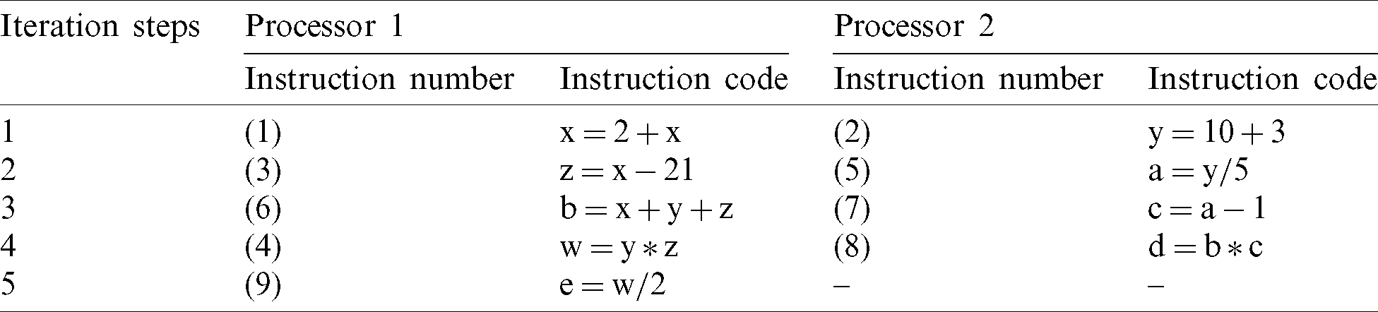
The data from Tab. 2 presents the results obtained after one iteration of the genetic algorithm and shows the chromosomes components and the corresponding fitness values. In Tab. 2, only a selection of the initial population is presented because there are a total of 150 chromosomes.
Table 2: Initial population—generation 0 (selection)
In Tab. 2, the fitness value was calculated according to the Paragraph 3.2 and the subparagraph named “Explanation of evaluation function”—( ). For the instructions presented in Fig. 3, the desired optimum is obtained after 3 iterations (
 ) and the chromosome corresponding to this optimum is: “8 6 7 2 4 5 0 9 1 3”.
Fig. 4 shows the distribution of instructions to the processors. In this figure, the symbol “–” means that there is no instruction to be executed. In the compressed solution, these symbols were removed.

Figure 4: Results obtained for first scenario
The evolution of fitness (best fitness) through the generations is depicted in Fig. 5. According to this figure, the desired fitness is obtained after three generations. The fitness value reflects the fact that all instructions were parallelized on the available processors.

Figure 5: Fitness evolution through generations
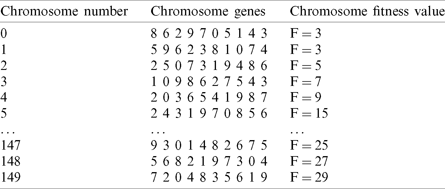
The second scenario: Program with nine instructions (as presented in Section 3.1). For this scenario, the input file has a block of nine instructions and the application main interface is presented in Fig. 6.
Figure 6: Application main interface—second scenario
For the instructions presented in Fig. 6, the desired optimum was obtained after 53 iterations ( ) and the chromosome corresponding to this optimum is: “ 0 4 10 6 7 9 8 15 16 1 2 13 5 3 17 11 14 12”.
Fig. 7 shows, accordingly with the chromosome shown above, the distribution of the instructions to the processors.

Figure 7: Results obtained for second scenario
The algorithms were coded in C# programming language, version 2015, and run on a Dell XPS L502X system with a configuration based on an i7-2630QM processor (frequency 2 GHz) and 8 GB RAM, and using the Microsoft Windows 10 PRO 64-bit operating system.
The evolution of fitness (best fitness) through the generations is depicted in Fig. 8. This figure indicates that the genetic algorithm achieves the desired fitness in an acceptable number of generations.
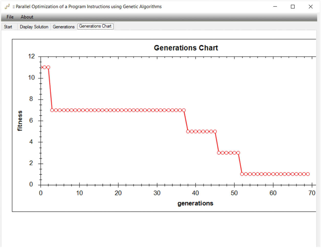
Figure 8: Fitness evolution through generations
Discussion. The problem of the optimal distribution of a set of instructions on the available processors, especially in today’s complex processors, is part of the NP-complete category. We showed through experiments that our genetic algorithm method is simple and efficient for implementation, because it is able to be scaled to a larger or smaller number of instructions that must be parallelized. Compared to the cellular automata variant presented in [27], our proposed solution is more efficient, because it is very difficult to use the knowledge acquired during the learning phase and transform it into cellular automata rules. As stated in [27], some questions are still open: e.g., What is the optimal cellular automata general structure? and How do we use the rules for new instances of the instruction scheduling task? In case of the local instruction scheduling presented in [18], the main problem was that the group of transformations that were applied to the data dependency graph imply adding edges, which adds constraints to the data dependency graph, and increases the runtime. The logic proposed in [19], injection of randomness in instruction scheduling list, can improve the efficiency in some cases, but there are also cases when the algorithm fails to produce efficient parallelization of instructions. In addition, this approach adds significant overhead to the process. All in all, the genetic algorithm-based method proposed in this research is generally scalable to a large number of instructions. The fact that instruction parallelizing works on varying number of instructions that must be scheduled means that the genetic algorithm is scalable. Our experimental results show that our method improves the exploration of the search space.
5 Conclusion and Possible Extensions to This Research
In this paper, we proposed a genetic algorithm to perform the parallelization of the instructions of a software program. The applicability and the efficiency of the proposed genetic algorithm in instruction scheduling is demonstrated by the experimental evaluation. The simulation results demonstrate that the solution based on genetic algorithms is suitable for this kind of problems and this approach can be used by compiler designers.
The steps we took to build our algorithm provide insight on how to further improve exploration of the search space. The results we obtained show that genetic algorithms are definitely worth investigating and represent a promising approach for future research. The logic used here to develop the genetic algorithm may be helpful with a few modifications to address other complicated parallelizing problems, such as parallelizing complex arithmetic instructions, and the treatment of cycles and decisions. In addition, it is possible to create a parallel version of the described algorithm, e.g., in a message passing interface, by using multiple computers or the IoT.
Funding Statement: The author received no specific funding for this study.
Conflicts of Interest: The author declare that they have no conflicts of interest to report regarding the present study.
1. J. L. Hennessy and T. R. Gross. (1982). “Code generation and reorganization in the presence of pipeline constraints,” in Proc. of the 9th ACM SIGPLANSIGACT Symp. on Principles of Programming Languages, Albuquerque, pp. 120–127. [Google Scholar]
2. P. K. Muhuri, A. Rauniyar and R. Nath. (2019). “On arrival scheduling of real-time precedence constrained tasks on multi-processor systems using genetic algorithm,” Future Generation Computer Systems, vol. 93, pp. 702–726. [Google Scholar]
3. G. De Micheli. (1994). Synthesis and Optimization of Digital Circuits, New York, United States: McGraw Hill. [Google Scholar]
4. S. G. Abraham, W. M. Meleis and I. D. Baev. (2000). “Efficient backtracking instruction schedulers,” in Proc. of the Int. Conf. on Parallel Architectures and Compilation Technique, Philadelphia, USA, pp. 301–308. [Google Scholar]
5. K. Wilken, J. Liu and M. Hefiernan. (2000). “Optimal instruction scheduling using integer programming,” in Proc. of the SIGPLAN Conf. on Programming Language Design and Implementation, Vancouver, pp. 121–133. [Google Scholar]
6. A. McGovern, J. E. B. Moss and A. G. Barto. (2002). “Building a basic block instruction scheduler using reinforcement learning and rollouts,” Machine Learning, vol. 49, no. 2–3, pp. 141–160. [Google Scholar]
7. J. E. B. Moss, P. E. Utgofi, J. Cavazos, D. Precup, D. Stefanovic et al. (1997). , “Learning to schedule straight-line code,” in Proc. of the 10th Conf. on Advances in Neural Information Processing Systems, Denver, USA, pp. 929–935. [Google Scholar]
8. D. Jimenez and C. Lin. (2001). “Perceptron learning for predicting the behavior of conditional branches,” in Proc. of the Int. Joint Conf. on Neural Networks, Washington, USA, pp. 2122–2126. [Google Scholar]
9. M. Stephenson, U. M. O’Reilly, M. C. Martin and S. Amarasinghe. (2003). “Genetic programming applied to compiler heuristic optimization,” Genetic Programming—EuroGP, vol. 2610, pp. 238–253. [Google Scholar]
10. M. Stephenson, S. Amarasinghe, M. C. Martin and U. M. O’Reilly. (2003). “Meta optimization: Improving compiler heuristics with machine learning,” ACM SIGPLAN Notices, vol. 38, no. 5, pp. 77–90. [Google Scholar]
11. S. Long and M. O’Boyle. (2004). “Adaptive java optimization using instance-based learning,” in Proc. of the 18th Annual Int. Conf. on Supercomputing, Saint-Malo, France, pp. 237–246. [Google Scholar]
12. G. Fursin, C. Miranda, O. Temam, M. Namolaru, E. Yom-Tov et al. (2008). , “MILEPOST GCC: Machine learning based research compiler,” in GCC Summit’08, Ottawa, Canada, pp. 1–13. [Google Scholar]
13. K. E. Coons, B. Robatmili, M. E. Taylor, B. A. Maher, D. Burger et al. (2008). , “Feature selection and policy optimization for distributed instruction placement using reinforcement learning,” in Int. Conf. on Parallel Architectures and Compilation Techniques, Toronto, Canada, pp. 32–42. [Google Scholar]
14. P. H. Sweany and S. J. Beaty. (1998). “Instruction scheduling using simulated annealing,” in Proc. of the 3rd Int. Conf. on Massively Parallel Computing Systems, Colorado Springs, USA. [Google Scholar]
15. K. E. Coons, X. Chen, D. Burger, K. S. McKinley and S. K. Kushwaha. (2006). “A spatial path scheduling algorithm for EDGE architectures,” in Proc. of the 12th Int. Conf. on Architectural Support for Programming Languages and Operating Systems, San Jose, pp. 129–140. [Google Scholar]
16. S. S. Muchnick. (1997). Advanced Compiler Design and Implementation, Burlington, Massachusetts, United States: Morgan Kaufmann Publishers Inc. [Google Scholar]
17. A. V. Aho, M. S. Lam, R. Sethi and J. D. Ullman. (2007). “Chapter 10—Compilers: Principles, techniques, and tools,” in Instruction-Level Parallelism, 2nd ed., Boston, Massachusetts, United States: Pearson/Addison Wesley. [Google Scholar]
18. M. Bahtat, S. Belkouch, P. Elleaume and P. Le Gall. (2016). “Instruction scheduling heuristic for an efficient FFT in VLIW processors with balanced resource usage,” EURASIP Journal on Advances in Signal Processing, vol. 38, no. 1, pp. 297. [Google Scholar]
19. G. Kouveli, K. Kourtis, G. Goumas and N. Koziris. (2019). “Exploring the benefits of randomized instruction scheduling,” . [Online]. Available: http://grow2011.inria.fr/media/papers/p3.pdf. [Google Scholar]
20. G. Tarsy and M. Woodard, “Method and apparatus for optimizing cost-based heuristic instruction schedulers,” US Patent #5,367,687, EP 0503928A3, filed 7/7/93, Granted 11/22/94.20G. [Google Scholar]
21. S. J. Beaty. (1991). “Genetic algorithms and instruction scheduling,” in Proc. of the 24th Int. Symp. on Microarchitecture, Portland, USA, pp. 206–211. [Google Scholar]
22. S. Beaty, S. Colcord and P. Sweany. (1999). “Using genetic algorithms to fine-tune instruction scheduling heuristics,” in Proc. of the Int. Conf. on Massively Parallel Computer Systems, Colorado Springs, USA. [Google Scholar]
23. V. H. Pham, N. H. Bui and N. B. Nguyen. (2014). “An approach to instruction scheduling at the processor architecture level for optimizing embedded software,” in Int. Conf. on Advanced Technologies for Communications, Hanoi, pp. 226–231. [Google Scholar]
24. M. Akbari, H. Rashidi and S. H. Alizadeh. (2017). “An enhanced genetic algorithm with new operators for task scheduling in heterogeneous computing systems,” Engineering Applications of Artificial Intelligence, vol. 61, pp. 35–46. [Google Scholar]
25. Z. Wang, Z. Ji, X. Wang, T. Wu and W. Huang. (2017). “A new parallel DNA algorithm to solve the task scheduling problem based on inspired computational model,” Biosystems, vol. 162, pp. 59–65. [Google Scholar]
26. S. Balin. (2011). “Non-identical parallel machine scheduling using genetic algorithm,” Expert Systems with Applications, vol. 38, no. 6, pp. 6814–6821. [Google Scholar]
27. F. Seredynski and A. Y. Zomaya. (2002). “Sequential and parallel cellular automata-based scheduling algorithms,” IEEE Transactions on Parallel and Distributed Systems, vol. 13, no. 10, pp. 1009–1023. [Google Scholar]
28. J. Holland. (1975). Adaptation in Natural and Artificial Systems, Michigan, United States: University of Michigan Press. [Google Scholar]
29. D. Goldberg. (1989). Genetic Algorithms in Search, Optimization, and Machine Learning, Boston, Massachusetts, United States: Addison-Wesley. [Google Scholar]
30. A. O. Fatma and M. A. Arafa. (2010). “Genetic algorithms for task scheduling problem,” Journal of Parallel and Distributed Computing, vol. 70, no. 1, pp. 13–22. [Google Scholar]
31. A. Y. Hamed, M. H. Alkinani and M. R. Hassan. (2020). “A genetic algorithm to solve capacity assignment problem in a flow network,” Computers, Materials & Continua, vol. 64, no. 3, pp. 1579–1586. [Google Scholar]
32. J. C. Potts, T. D. Giddens and S. B. Yadav. (1994). “The development and evaluation of an improved genetic algorithm based on migration and artificial selection,” IEEE Transactions on Systems, Man, and Cybernetics, vol. 24, no. 1, pp. 73–86. [Google Scholar]
 | This work is licensed under a Creative Commons Attribution 4.0 International License, which permits unrestricted use, distribution, and reproduction in any medium, provided the original work is properly cited. |