DOI:10.32604/cmc.2021.015426
| Computers, Materials & Continua DOI:10.32604/cmc.2021.015426 | |
| Article |
Energy-Efficient Transmission Range Optimization Model for WSN-Based Internet of Things
1Department of Computer Science and Engineering, Sejong University, Seoul, Korea
2Department of Electronics and Communication Engineering, D.B.R.A. National Institute of Technology, Jalandhar, India
3SCMS School of Engineering and Technology, Ernakulam, India
4Department of Electronics Engineer, Kyung Hee University, Yongin, Korea
*Corresponding Author: Doug Young Suh. Email: suh@khu.ac.kr
Received: 02 November 2020; Accepted: 10 December 2020
Abstract: With the explosive advancements in wireless communications and digital electronics, some tiny devices, sensors, became a part of our daily life in numerous fields. Wireless sensor networks (WSNs) is composed of tiny sensor devices. WSNs have emerged as a key technology enabling the realization of the Internet of Things (IoT). In particular, the sensor-based revolution of WSN-based IoT has led to considerable technological growth in nearly all circles of our life such as smart cities, smart homes, smart healthcare, security applications, environmental monitoring, etc. However, the limitations of energy, communication range, and computational resources are bottlenecks to the widespread applications of this technology. In order to tackle these issues, in this paper, we propose an Energy-efficient Transmission Range Optimized Model for IoT (ETROMI), which can optimize the transmission range of the sensor nodes to curb the hot-spot problem occurring in multi-hop communication. In particular, we maximize the transmission range by employing linear programming to alleviate the sensor nodes’ energy consumption and considerably enhance the network longevity compared to that achievable using state-of-the-art algorithms. Through extensive simulation results, we demonstrate the superiority of the proposed model. ETROMI is expected to be extensively used for various smart city, smart home, and smart healthcare applications in which the transmission range of the sensor nodes is a key concern.
Keywords: Internet of Things; wireless sensor networks; routing; transmission range optimization; energy-efficiency; hot-spot problem; linear programming
1.1 Background and Problem Statement
Data-driven wireless sensor networks (WSNs) are widely applied to enhance the Internet of Things (IoT) in terms of the data throughput, energy efficiency, and self-management [1]. WSN-based IoTs are composed of wireless sensor nodes, which realize data collection and communication [2,3]. In this framework, the sensor nodes are deployed in the physical environment to sense the phenomena and report their readings in a distributed manner to the sinks [4]. However, the sensor nodes exhibit certain limitations in terms of energy, computation resources, and communication range [5,6].
When a WSN-based IoT is deployed over a large application area, the nodes perform multihop communication due to the limited transmission range, and direct data transmission cannot be realized. Furthermore, it has been reported that a larger number of relay nodes on the path of data delivery to the sink corresponds to a higher probability of these nodes closer to the sink suffering from hot-spot problem [7]. In such a scenario, the number of intermediate nodes should be reduced to decrease the emergence of a no-connection zone for distantly located nodes.
Moreover, the battery of the sensor nodes may not be able to be changed or recharged. Therefore, it is necessary to ensure efficient power consumption in a WSN-based IoT [8]. Furthermore, transmitting one kilobyte of data corresponds to the processing of three million instructions [9]. Therefore, data transmission in the WSNs should be minimized with regard to the distance between any two entities among sensor nodes, cluster heads (CHs), or sinks [10].
One solution is to maximize the transmission range between nodes. The key concept of transmission range maximization is that if a sensor initiates a data packet transmission to a sink located 1000 m away, the least number of relay sensors should be selected to forward the packet. The communication range of sensor nodes depends on their transmission power and the volume of the packet to be transmitted. Transmission over long distances requires a higher energy [11,12]. Therefore, it is necessary to determine the maximum possible distance (transmission range) to which the sensor nodes can transmit the data packets.
Many researchers have attempted to reduce the energy consumption by avoiding the hot-spot problem [13]. In particular, Verma et al. [14] proposed the multiple sink-based genetic algorithm-based optimized clustering (MS-GAOC) approach, in which four data collection sinks were incorporated outside the network. However, the cost of using four sinks may be prohibitive in various applications.
Moreover, researchers generally apply the corona-based model to avoid hot-spot problems. A survey of the various corona-based approaches has been presented in an existing study [15]. Nevertheless, even corona-based methods are not sufficiently reliable in mitigating the hot-spot problem. In fact, the literature review indicates that the concept of transmission range adjustment for the sensor nodes, to realize direct data transfer to the sink or transfer with the least possible number of intermediate nodes, has not been extensively investigated.
The review pertaining to the mitigation of hot-spot problems indicated that the optimization-based approach can provide a balanced solution to specific problems. Therefore, in this work, we used linear programming (LP) to compute the maximum data transmission range [16,17]. In particular, LP exhibits remarkable exploration and exploitation capabilities, enabling fast convergence to the optimal solution. Moreover, LP is highly computationally efficient [16].
In the context of the aforementioned problems, the key contributions of this work are as follow:
a) We propose an energy-efficient transmission range optimized model for IoT (ETROMI) to optimize the transmission range of the sensor nodes to reduce the hot-spot problem in WSN-based IoT.
b) The mathematical model and formulation using LP is presented.
c) The simplex method is used to solve the defined problem.
d) The proposed model’s performance of the proposed model is analyzed in terms of various aspects, and the optimal solution is identified.
The remaining paper is structured as follows. Section 2 presents the background of transmission range adjustment algorithms and describes the existing work pertaining to the hot-spot problem in WSNs. Section 3 describes the system model and explains the LP formulation. Section 4 describes the performance evaluation of ETROMI, which is used to compute the maximized distance corresponding to the transmission range of a node. The concluding remarks, along with the limitations and scope for future work, are presented in Section 5.
In this section, we discuss the existing work focused on addressing the hot-spot problem through various state-of-the-art techniques and on realizing the transmission range adjustment of a sensor node.
2.1 Approaches to Solve the Hot-Spot Problem
In applications involving an extremely large network area, the sensor nodes inevitably perform multi-hop communication [18]. In this process, a hot-spot is created at the nodes located nearest to the sink. Several researchers have addressed this concern through various topology-based methods. Moreover, the many-to-one approach (many sensor nodes corresponding to one sink) has been widely implemented through corona-based structures [13]. Many researchers use the term “energy-hole,” which is equivalent in meaning to a hot-spot.
Elkamel et al. [19] proposed an unequal clustering method to overcome the hot-spot problem by placing the small and large clusters nearer to and farther from the sink, respectively. However, the proposed technique failed to eliminate the hot-spot problem, and the network’s energy consumption was high. Verma et al. [7,14] implemented multiple data sinks in a given network to mitigate the hot-spot problem. In their former and latter studies, the authors used the conventional approach and the genetic algorithm, respectively. However, the network incurred a higher financial cost owing to the use of multiple data sinks. The authors in [20] proposed a virtual-force-based energy-hole mitigation strategy to ensure sensor nodes’ uniform distribution. Moreover, the network was composed of various annuli, and virtual gravity was used to optimize the sensor node positions in each annulus. However, due to the multi-hop communication, the number of overheads in each annulus was extremely high, which increased the energy consumption in the network. Sharmin et al. [21] proposed a strategy in which the network was partitioned into several wedges, and residual energy was considered to combine the various wedges. The head node was selected based on the distance between the innermost corona and node. However, the inefficient selection of the head node led to the mediocre performance of this strategy.
In addition to the static network scenario, certain researchers introduced sink mobility to curb the hot-spot problem. Sahoo et al. [22] proposed a particle-swarm-optimization-based energy-efficient clustering and sink mobility (PSO-ECSM) technique, in which the sink mobility was used to alleviate the hot-spot problem. However, the mobility scenario was not efficiently utilized, and the slow convergence of the PSO degraded the performance of the proposed scheme. Furthermore, Kaur et al. [23] introduced dual sink mobility outside the network to target unattended applications. Although the authors implemented the PSO-based sink mobility, the use of the dual sink introduced overheads in the network, which increased the energy consumption. In addition, the data delivery was required to be synchronized when using the two sinks in the network. Certain other researchers also employed the sink mobility scenario to alleviate the hot-spot problem. However, it was observed that the use of sink mobility limited the applicability of the approaches in various real-time scenarios.
2.2 Transmission Range Adjustment Algorithms
In addition to the network topological changes associated with the introduction of the corona-based model, the characteristics of sensor nodes have been examined. The focus of the present study is to optimize the transmission range. Although certain researchers have attempted to adjust the transmission range to alleviate the hot-spot problem, the proposed approaches suffer from the inherent problems, which limit their relevance.
In an existing strategy [24] pertaining to the transmission range adjustment, the network was divided into various concentric sets termed as coronas. Every corona was assigned a transmission range level. Furthermore, the authors presented an ant colony optimization (ACO)-based transmission range adjustment strategy [24] to prolong the network lifetime. Liu [25] considered the energy consumption balancing (ECB) and energy consumption minimization (ECM) techniques to avoid the occurrence of energy holes. The authors exploited the short-trip moving scheme for the ACO, which helped in decreasing the complexity and in the amelioration of convergence speed. Furthermore, the authors considered a reference transmission distance to implement the ECB and ECM techniques. Xin et al. [26] were the first to attempt to solve the many-to-one data transmission problem, particularly in strip-based WSNs. The authors adjusted the transmission range based on the computation of the accurate distance. The objective was to prolong the network lifetime. However, the proposed algorithm was applicable only for strip-based WSNs, for example, railway track, bridge, and tunnel systems.
In summary, only a few studies have been focused on addressing the hot-spot problem through transmission range adjustment, and this approach exhibits considerable scope for improvement. Furthermore, the use of LP for energy-hole mitigation in the transmission range adjustment context is yet to be explored. Therefore, we implement these aspects in our proposed strategy.
In this section, we describe the network assumptions and the system model.
The following network assumptions are considered to implement ETROMI.
a) The WSN is composed of one sink and several sensor nodes that collect data and transfer them to the sink.
b) Each sensor has a unique ID.
c) There is no dispute for medium access, and thus, proportional fair channel access is available to all the sensors.
d) The minimum cost forwarding approach is employed as the multi-hop-routing protocol.
e) The sensor nodes are homogeneous, i.e., all the nodes have the same configuration in terms of energy, computational resources, transmission range, etc.
f) The entire network is static, including the CHs and the sink.
g) The entire network has ideal conditions in terms of security, physical medium factors, reflection, refraction, splitting of signals, and presence of other obstacles.
3.2 Fundamental Principle of ETROMI
Assume a WSN with N sensor nodes, in which one of the sensor nodes initiates a data packet with the intent to transmit it to the sink (final receiver base station). In the conventional clustering method, a CH collects the data from the sensors node in the corresponding cluster and forwards the data toward the sink via the other CHs. However, this approach is not efficient because the CHs suffer from battery limitations, even more than the other data collecting elements, but must be involved in all transmissions.
In contrast, the lifetime of the WSNs depends on the remaining energy of the members, i.e., the sensor nodes. Therefore, the number of forwarding nodes must be minimized. In this study, we assume that instead of always selecting the CHs to receive and forward the data packets, the sensors select the farthest sensor node in their transmission range. In other words, the sensor nodes increase their transmission power to transmit a data packet over a longer distance. In this configuration, the number of nodes that are involved in a transmission are minimized, which can considerably improve the energy efficiency. In Fig. 1, the red dotted line represents the routing procedure in a clustering-based method.

Figure 1: Routing procedure in WSNs
In this approach, the nodes send their packets to their corresponding CH, which then forwards the packet to the next CH and so on. Finally, the closest CH delivers the packet to the sink. In contrast, in the approach represented by the green dashed line, the node that initiates the packet sends the packet to the farthest node, and the receiver node follows the same principle and send the packet to the farthest node in its transmission range. Consequently, the number of nodes involved in the transmission procedure is less than that in the clustering-based method.
Consider a network involving 100 sensor nodes. Sensor 1 initiates a data packet and wants to send it to node 100. As mentioned earlier, in the WSNs, the topology is multi-hop. In other words, node 1 sends its packet to its neighbor, which receives the packet and forwards it to the neighboring nodes, excluding the node that the packet was received from. This process continues until node 100 receives the packet. The problem then is to determine the number of nodes in the transmission process that receive and forward the packet. This number of the relay nodes should be minimized to abate the energy consumption and, in turn, prolongs the network lifetime.
One solution is to increase the transmission range of the nodes involved in the transmission process from the source to the destination. In this case, a node selects a neighboring node, which is far from it, but in its range, i.e., on the edge of its transmission range, and the number of intermediate nodes is decreased. To this end, we consider the energy consumption accounted to transmission and reception of data packets and also the magnitude of data packets. The total required energy can be expressed as

The list of main symbols used in this paper are listed in Tab. 1.

Consider a WSN-based IoT represented by graph  , in which
 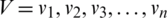 is the set of sensor nodes, and
  is the set of direct wireless links between the nodes, such that
  . Link
  exists if and only if
  , where Li is the set of all nodes that can be reached by sensor i directly with a certain transmission power level. Furthermore, each sensor i has the initial power EI. The transmission energy consumed by node i to send a data packet to the neighboring sensor j is
  ;
;  is the energy required for a node to receive a packet from node i; and
  is the set of the packet volumes.
The objective function is to maximize the transmission distance with respect to the packet volume and the transmission and receiving energies, that is


Constraint (3) specifies that the total number of packets received or transmitted to/from node i must be less than a threshold for a specific time slot. Constraints (4) and (5) control the maximum transmission and receiving energy consumptions, respectively. Constraint (6) ensures that the total consumed energy for transmission and receiving by node i, is not less than the initial energy of the node.
To evaluate the performance of the technique, we consider that a data packet is to be sent from a sensor node to the sink via two intermediate sensor nodes. Therefore, four sensor nodes are involved in the process: one sender, one sink, and two relay nodes. The size of each packet is 50 bits, and the transmission and receiving power are 100 and 70 W, respectively.
The linear problem can be expressed as


By adding slack variables to constraints, the primal problem in standard format is represented as follows:


We use the simplex method to solve the problem. The simplex method is used to solve LP models by using slack variables, tableaus, and pivot variables to determine the optimal solution of an optimization problem [27]. To solve the optimization problem, the following steps are performed:
a) Obtain the standard form,
b) Introduce slack variables,
c) Create the tableau,
d) Identify the pivot variables,
e) Create a new tableau,
f) Check for optimality,
g) Identify the optimal values.
The procedure starts with an initialization phase, followed by several iterations to determine the optimal solution.
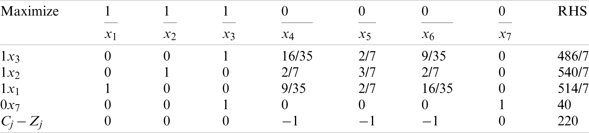
The initialization step for our optimization problem is presented in Tab. 2. After the first step, x6 is the leaving variable, x1 is the entering variable, and 4 is the pivot element.

Subsequently, we apply the first iteration, as indicated in Tab. 3. Upon completing this iteration, the leaving variable is x5, the entering variable is x2, and the pivot element is 4.

We continue by applying the second iteration as indicated in Tab. 4, which results in a leaving variable x4, an entering variable x3, and a pivot element, 35/16.

We proceed to the third iteration, in which all Cj − Zj values are zero or negative; therefore, the simplex method is terminated at this step, as indicated in Tab. 5. The optimal solution for the defined problem is presented in Tab. 6.


The duality refers to a specific relationship between an LP problem and another problem, both of which involve the same original data, albeit located differently [28]. The former and latter problems are referred to as the primal and dual problems, respectively. The feasible regions, optimal solutions, and optimal values of these problems must be strongly correlated. The duality and optimality conditions obtained from these aspects are a basis for the LP theory. Once either of the primal or dual problems is solved, both the problems can be solved owing to duality. To convert the primal problem to a dual problem, the following steps are performed:
a) If the primal problem corresponds to “Maximize,” the dual problem corresponds to “Minimize.”
b) The number of variables in the dual problem is equal to the number of constraints in the primal problem.
c) The number of constraints in the dual problem, is equal to the number of variables in the primal problem.
d) The coefficients of the objective function in the dual problem, are equal to the right-hand side (RHS) values in the primal problem.
e) The RHS values in the dual problem are equal to the coefficients of the objective function in the primal problem.
f) The coefficient variables in the constraints of the dual problem correspond to the transpose matrix of the coefficient variables in the primal problem.
g) “ ” constraints in the primal problem are “
 ” constraints in the dual problem, and vice versa.
h) The variables in the dual problem are denoted as “y”.
i) The objective function is denoted as “w”. The primal problem is as follows:
Our primal problem is as below:


Coefficient matrix of basic variables in objective function is  , Coefficient matrix of basic variables in constraints is
  , and RHS matrix is
  . Based on the aforementioned steps, our dual problem will be as bellow:


By adding surplus variables, the dual problem is as follows:


As indicated in the dual problem, no identity matrix exists for the coefficients of the variables in the constraints; therefore, artificial variables must be introduced. In this case, the dual problem in the standard format is:


By adding artificial variables, an identity matrix can be generated, and the simplex method can be implemented.
As indicated in Tab. 7, after completing the initialization section, the leaving variable is a3, the entering variable is x1, and the pivot element is 4. Subsequently, we implement the first iteration, as indicated in Tab. 8. Upon completing iteration I, the leaving variable is a2, the entering variable is x2, and our pivot element is 4. We then proceed to the second iteration, as indicated in Tab. 9. After the second iteration, the leaving variable is a1, the entering variable is x3, and the pivot element is 35/16. We attempt to determine the optimal solution by using the two-phase simplex method. All the artificial variables are removed, and the problem can be solved through the other variables. We then apply the third iteration in two phases, as indicated in Tabs. 10 and 11.

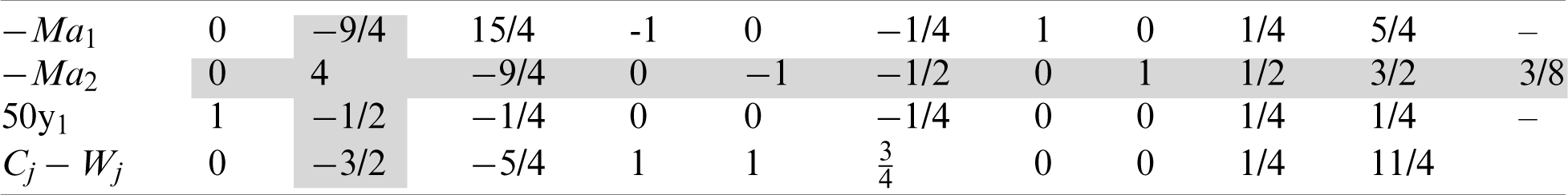

Table 10: Phase I, Iteration III

Table 11: Phase II, Iteration III

Finally, it is observed that the primal solution, presented in Tab. 12, is equal to the dual solution, presented in Tab. 13, that is Z* = W*.
Table 12: Primal optimal Solution

Table 13: Dual optimal solution
Sensitivity analysis is aimed at examining the influence of changes in the variables, such as the RHS, coefficients of the objective function, and constraints, on the solution. We start with Tab. 14 and make the some changes as explained in the next subsection.
Table 14: Simplex optimum tableau

4.4.1 Change in the Objective Function Coefficient for Non-Basic Variables
In the last iteration, no non-basic variables of the objective function exist. Therefore, if one of the coefficients is changed, the optimal solution is not influenced.
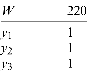
Suppose the intention is to change the first RHS to b1; then we have  . To calculate new RHS;
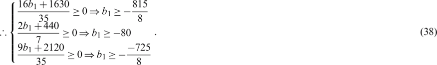
Because,  8. We suppose a b1 value beyond the specified range; as an example −110.
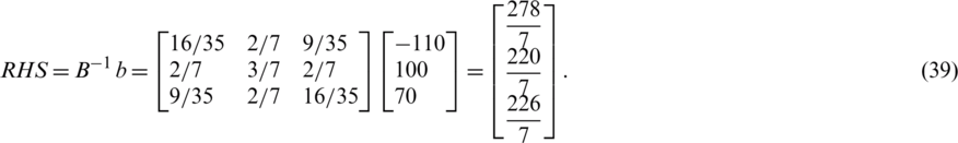
Now, we continue the tableau with new RHS values;
As indicated in Tab. 15, the primal solution is not feasible; therefore, we attempt to find the optimal solution through the dual problem.

The initialization step, as the first iteration, is presented in Tab. 16. After completing the initialization step, the leaving variable is x1, the entering variable is x5, and the pivot element is 3/7.

Subsequently, we implement the second iteration, as indicated in Tab. 17. After finishing the second iteration, it is noted that the primal is feasible; the leaving variable is x5, the entering variable is x2, and the pivot element is 7/3.
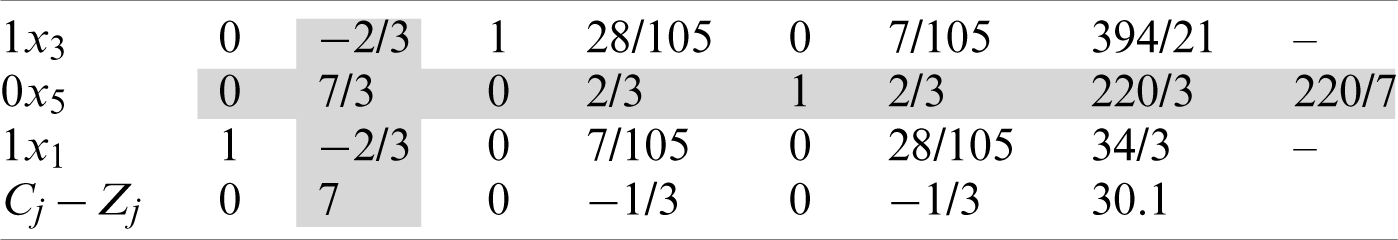
We then implement the third iteration as indicated in Tab. 18. All the values for Cj − Zj are zero or negative; therefore, the process is terminated at this step. The optimal solution is as presented in Tab. 19.

4.4.3 Change in the Objective Function Coefficient for the Basic Variable
We consider the case in which the coefficient of x1 changes. Suppose the coefficient of x1 is c1.
Any change in the coefficient of the basic variables of the objective function affects the value of Cj − Zj.


If  then the present solution remains optimal solution;


In this case, the range of c1 is greater than −26/9. Thus, we assign c1 beyond this range, for example c1 = −4, and implement the first iteration, as indicated in Tab. 20.

Upon completing the first iteration, the leaving variable is x3, the entering variable is x6, and the pivot element is 9/35.
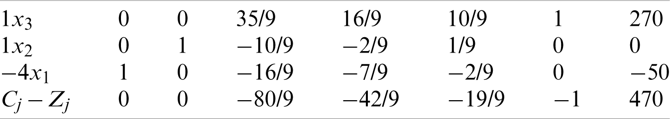
The second iteration is presented in Tab. 21. All the values for Cj − Zj are zero or negative; therefore, the process is terminated at this step. We conclude that the optimal solution is as follows: x1 = −50, x2 = 0, x3 = 270 and z = 470.
4.4.4 Change in the Constraint Coefficient Corresponding to Non-basic Variables
In the last iteration, no non-basic variable of the objective function exists. Therefore, if one of the coefficients is changed, the optimal solution is not influenced.
4.4.5 Addition of a New Variable
Consider a new variable x7 with coefficient c7 = 12 and  , then;
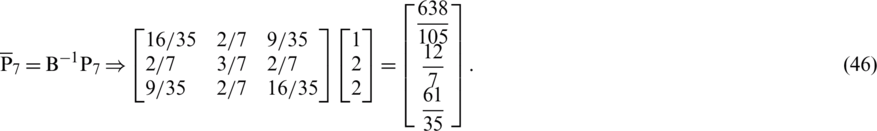
In this case, we perform three iterations as indicated in Tabs. 22–24.

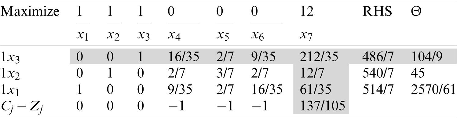
Upon completing the first iteration, the leaving variable is x3, the entering variable is x7, and the pivot element is 212/35.
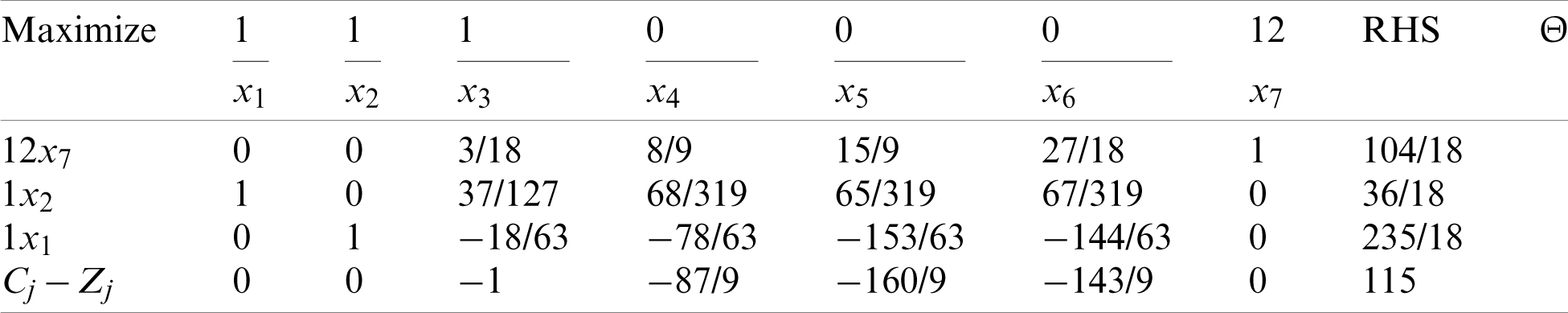
The third iteration is presented in Tab. 12, in which all the values for Cj − Zj are zero or negative and; therefore, the program is terminated at this step, and the optimal solution is as indicated in Tab. 25.
4.4.6 Addition of a New Constraint
To examine the influence of the addition of a new constraint to the problem, we consider  :
:
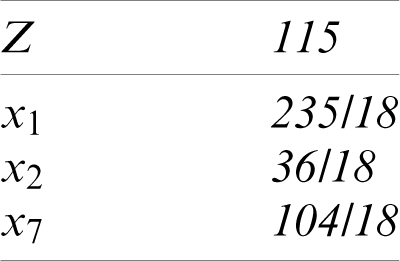
As indicated in Tab. 26, the optimal solution is as follows: x1 = 514/7, x2 = 540/7, x3 = 486/7, and Z = 20.
Table 26: Additional constraint
5 Conclusion and Future Direction
The transmission range of a sensor node defines whether the communication mode is single-hop or multi-hop. In this paper, we proposed the use of ETROMI, which can determine the maximum distance to which a sensor node can transmit data with the least possible number of relay nodes. We presented an LP-based analytical model to determine the transmission range of the sensor node. Moreover, we explained the mathematical model associated with the ETROMI to reduce the energy consumption of WSN-based IoT. A key concern about the ETROMI is that it considers the ideal conditions involving no obstacles between the sensor nodes and the sink. Therefore, the model performance is specific to the circumstances. Furthermore, the network is assumed to be homogeneous, whereas homogeneity does not exist in an actual network due to the different factors associated with network deployment. In future work, we aim to extend our work to address the aforementioned scenarios.
Funding Statement: This research was supported by Korea Electric Power Corporation (Grant Number: R18XA02).
Conflicts of Interest: The authors declare that they have no conflicts of interest to report regarding the present study.
1. S. Kumar and V. K. Chaurasiya. (2018). “A strategy for elimination of data redundancy in Internet of Things (IoT) based wireless sensor network (WSN),” IEEE Systems Journal, vol. 13, pp. 1650–1657. [Google Scholar]
2. P. Swarna, P. Maddikunta, M. Parimala, S. Koppu, T. Gadekallu et al. (2020). , “An effective feature engineering for DNN using hybrid PCA-GWO for intrusion detection in IoMT architecture,” Computer Communications, vol. 160, pp. 139–149. [Google Scholar]
3. R. Vinayakumar, M. Alazab, S. Srinivasan, Q. Pham, S. Padannayil et al. (2020). , “A visualized botnet detection system based deep learning for the Internet of Things networks of smart cities,” IEEE Transactions on Industry Applications, vol. 56, no. 4, pp. 4436–4456. [Google Scholar]
4. M. Piran, Y. Cho, J. Yun and D. Y. Suh. (2014). “Cognitive radio-based vehicular ad hoc and sensor networks (CR-VASNET),” International Journal of Distributed Sensor Networks, vol. 2014, pp. 1–11. [Google Scholar]
5. T. M. Behera, S. K. Mohapatra, U. C. Samal and M. S. Khan. (2019). “Hybrid heterogeneous routing scheme for improved network performance in WSNs for animal tracking,” Internet of Things, vol. 6, pp. 1–9. [Google Scholar]
6. T. M. Behera, S. K. Mohapatra, U. C. Samal, M. S. Khan, M. Daneshmand et al. (2019). , “Residual energy-based cluster-head selection in WSNs for IoT application,” IEEE Internet of Things Journal, vol. 6, pp. 5132–5139. [Google Scholar]
7. S. Verma, N. Sood and A. K. Sharma. (2019). “A novelistic approach for energy efficient routing using single and multiple data sinks in heterogeneous wireless sensor network,” Peer-to-Peer Networking and Applications, vol. 12, pp. 1110–1136. [Google Scholar]
8. Y. Liu, C. Yang, L. Jiang, S. Xie and Y. Zhang. (2019). “Intelligent edge computing for IoT-based energy management in smart cities,” IEEE Network, vol. 33, pp. 111–117. [Google Scholar]
9. D. K. Gupta. (2013). “A review on wireless sensor networks,” Network and Complex Systems, vol. 3, no. 1, pp. 18–23. [Google Scholar]
10. L. Krishnasamy, R. K. Dhanaraj, G. D. Ganesh, G. Reddy, M. K. Aboudaif et al. (2020). , “A heuristic angular clustering framework for secured statistical data aggregation in sensor networks,” Sensors, vol. 20, pp. 1–15. [Google Scholar]
11. S. Bhattacharya, P. Maddikunta, S. Somayaji, K. Lakshmanna, R. Kaluri et al. (2020). , “Load balancing of energy cloud using wind driven and firefly algorithms in internet of everything,” Journal of Parallel and Distributed Computing, vol. 142, pp. 16–26. [Google Scholar]
12. C. Iwendi, P. K. Maddikunta, T. R. Gadekallu, K. Lakshmanna, A. K. Bashir et al. (2020). , “A metaheuristic optimization approach for energy efficiency in the IoT networks,” Software: Practice and Experience, vol. 22, no. 6, pp. 1–14. [Google Scholar]
13. H. Asharioun, H. Asadollahi, T. C. Wan and N. Gharaei. (2015). “A survey on analytical modeling and mitigation techniques for the energy hole problem in corona-based wireless sensor network,” Wireless Personal Communications, vol. 81, pp. 161–187. [Google Scholar]
14. S. Verma, N. Sood and A. K. Sharma. (2019). “Genetic algorithm-based optimized cluster head selection for single and multiple data sinks in heterogeneous wireless sensor network,” Applied Soft Computing, vol. 85, pp. 1–21. [Google Scholar]
15. A. U. Rahman, A. Alharby, H. Hasbullah and K. Almuzaini. (2016). “Corona based deployment strategies in wireless sensor network: A survey,” Journal of Network and Computer Applications, vol. 64, pp. 176–193. [Google Scholar]
16. D. Bertsimas and J. N. Tsitsiklis. (1997). Introduction to Linear Optimization, vol. 6. Belmont, MA: Athena Scientific. [Google Scholar]
17. V. Tabus, D. Moltchanov, Y. Koucheryavy, I. Tabus and J. Astola. (2015). “Energy efficient wireless sensor networks using linear-programming optimization of the communication schedule,” Journal of Communications and Networks, vol. 17, pp. 184–197. [Google Scholar]
18. V. Sandeep, N. Sood and A. K. Sharma. (2019). “QoS provisioning-based routing protocols using multiple data sink in IoT-based WSN,” Modern Physics Letters, vol. 34, pp. 1–36. [Google Scholar]
19. R. Elkamel, A. Messouadi and A. Cherif. (2019). “Extending the lifetime of wireless sensor networks through mitigating the hot spot problem,” Journal of Parallel and Distributed Computing, vol. 133, pp. 159–169. [Google Scholar]
20. C. Sha, C. Ren, R. Malekian, M. Wu, H. Huang et al. (2019). , “A type of virtual force-based energy-hole mitigation strategy for sensor networks,” IEEE Sensors Journal, vol. 20, pp. 1105–1119. [Google Scholar]
21. N. Sharmin, A. Karmaker, W. Lambert, M. Alam and M. Shawkat. (2020). “Minimizing the energy hole problem in wireless sensor networks: A wedge merging approach,” Sensors, vol. 20, pp. 1–25. [Google Scholar]
22. B. Sahoo, T. Amgoth and H. Pandey. (2020). “Particle swarm optimization based energy efficient clustering and sink mobility in heterogeneous wireless sensor network,” Ad Hoc Networks, vol. 106, pp. 1–21. [Google Scholar]
23. S. Kaur and V. Grewal. (2020). “A novel approach for particle swarm optimization-based clustering with dual sink mobility in wireless sensor network,” International Journal of Communication Systems, vol. 33, no. 16, pp. 1–23. [Google Scholar]
24. M. Liu and C. Song. (2012). “Ant-based transmission range assignment scheme for energy hole problem in wireless sensor networks,” International Journal of Distributed Sensor Networks, vol. 8, pp. 1–12. [Google Scholar]
25. X. Liu. (2016). “A novel transmission range adjustment strategy for energy hole avoiding in wireless sensor networks,” Journal of Network and Computer Applications, vol. 67, pp. 43–52. [Google Scholar]
26. H. Xin and X. Liu. (2017). “Energy-balanced transmission with accurate distances for strip-based wireless sensor networks,” IEEE Access, vol. 5, pp. 16193–16204. [Google Scholar]
27. V. Zhadan. (2019). “Two-phase simplex method for linear semidefinite optimization,” Optimization Letters, vol. 13, pp. 1969–1984. [Google Scholar]
28. S. Nasseri and D. Darvishi. (2018). “Duality results on grey linear programming problems,” The Journal of Grey System, vol. 30, pp. 127–142. [Google Scholar]
 | This work is licensed under a Creative Commons Attribution 4.0 International License, which permits unrestricted use, distribution, and reproduction in any medium, provided the original work is properly cited. |