DOI:10.32604/cmc.2021.015402
| Computers, Materials & Continua DOI:10.32604/cmc.2021.015402 | |
| Article |
An Energy-Efficient Mobile-Sink Path-Finding Strategy for UAV WSNs
Department of Computer and Communication Technology, Faculty of Information and Communication Technology, Universiti Tunku Abdul Rahman, Perak, 31900, Malaysia
*Corresponding Author: Lyk Yin Tan. Email: tanlyky@utar.edu.my
Received: 19 November 2020; Accepted: 19 December 2020
Abstract: Data collection using a mobile sink in a Wireless Sensor Network (WSN) has received much attention in recent years owing to its potential to reduce the energy consumption of sensor nodes and thus enhancing the lifetime of the WSN. However, a critical issue of this approach is the latency of data to reach the base station. Although many data collection algorithms have been introduced in the literature to reduce delays in data delivery, their performances are affected by the flight trajectory taken by the mobile sink, which might not be optimized yet. This paper proposes a new path-finding strategy, called Energy-efficiency Path-finding Strategy (EPS) in the Air-Ground Collaborative Wireless Sensor Network (AGCWSN). The proposed approach is able to greatly enhance the efficiency of data collection. The performance of the proposed strategy is simulated and compared with the existing strategies over several parameters. The simulation results show that the mobile sink with EPS can collects data with lower data delivery delay as compared to other existing strategies. The number of data retransmissions between sensor nodes and mobile sink in EPS is also the lowest in EPS among several existing strategies. The data delivery delay is 66% and 120% lower than Rest Center Tractor Scanning (RCTS) and Non-stop Center Tractor Scanning (NCTS) in irregular and grid topology respectively. The data delivery delay is 62% lower than Two Row Scanning (TRS) in grid topology and 120% lower than RkM in irregular topology. The packet loss of EPS-2 is 1.3% lower than RkM.
Keywords: Wireless network; mobile sink; efficient path; data collection
Wireless Sensor Network (WSN) has revealed great potential in a wide range of applications such as agribusiness, military, health care, environmental etc. [1–3]. WSN is a wireless network consists of spatially distributed autonomous devices with inbuilt sensors, called sensor nodes to monitor physical or environmental information of a targeted area [4]. The low-power and inexpensive sensor nodes are equipped with small data processing unit, limited memory unit, constrained transmission range transceiver, and finite available energy [5,6]. With the equipped components, the sensor nodes are able to sense the environmental attributes and forward the sensed data to a base station. Typically, such data forwarding is carried out through multi-hop communication as shown in Fig. 1 [7].

Figure 1: Multi-hop communication of WSN [7]
In multi-hop communication, the sensor nodes which are close to the base station prone to experience traffic congestion because they act as the relay nodes to forward the sensed data from other sensor nodes to the base station. As a result, the nearer a sensor node is to the base station, generally the more quickly its energy is depleted. While the energy of a sensor node is depleted, the communication linkage between the base station and some sensor nodes could be broken, leaving the base station unreachable from these sensor nodes and thus interrupting the data collection process. In the literature, this situation is named as the energy hole problem, which is also referred to as the uneven sensor nodes’ energy depletion phenomenon in the sensed area [8].
The energy hole problem is one of the critical challenges in enhancing network lifetime for WSN using multihop communication [9]. To resolve the issue, a mobile sink approach has then been introduced where a mobile sink is scheduled to move around in the WSN to collect sensed data directly from sensor nodes so as to improve load balancing among the sensor nodes [10]. After collecting the data, the mobile sink will have to return to the base station in order to offload the data and charge its battery. Due to the vehicle capability, the weight carried by the mobile sink and thus the battery capacity are limited. Therefore, the duration of a round of data collection by the mobile sink in the sensed area is quite tight [11]. To enhance the efficiency of data collection in WSN, the energy (battery capacity) used by the mobile sink needs to be optimized [12,13].
In general, there are two possibilities to implement a mobile sink—Using a ground or an aerial vehicle. However, there are several disadvantages of using a ground vehicle for data collection in a WSN, especially when the terrain is unstructured and with obstacles. For example, the sensed area is located inside a forest which creates difficulty for the ground mobile sink to move; or a river lies between the base station and the sensed area which isolates the base station from the sensed area. To avoid the above-mentioned problems, this paper studies the approach that uses an aerial mobile sink for data collection in WSN. Such a WSN is also known as the Air-Ground Collaborative Wireless Sensor Network (AGCWSN).
We propose an Energy-efficiency Path-finding Strategy (EPS) for AGCWSN to enhance the efficiency in data collection. Basically, an aerial mobile sink in an AGCWSN will be flying through several data collection points to collect data [14]. Rather than each data collection point covers only one sensor node, we further propose that Intermediate Points (IPs) can be pre-defined so that each of them covers several sensor nodes rather than one. That is, when the mobile sink passes by an IP, the sensor nodes within the transmission range will upload the sensed data to the mobile sink by single-hop transmission. Moreover, the entire set of IPs should cover all the sensor nodes in the sensed area. Throughout study and simulation, if a proper set of IPs and the corresponding fairly good flying path can be identified, EPS is able to effectively reduce the mobile sink’s flight distance. Since the time needed to create the best flight trajectory is increased exponentially when the number of IPs increases, the Genetic Algorithm (GA) is used to compute an acceptable flight trajectory to avoid a long waiting time for flight trajectory generation [15].
The remaining of the paper is organized as follows. Section 2 presents a background review of existing AGCWSN algorithms. A design of EPS is exhibited in Section 3. Simulation results are shown and discussed in Section 4. Lastly, Section 5 concludes our work.
Traditionally a WSN is formed by a number of sensor nodes and a static sink where the sensor nodes forward sensed data to the static sink wirelessly in the sensed area. A multi-hop routing protocol is needed in data collection when the distance between the sensor nodes and the static sink exceeds the transmission range [10]. Hence, it triggers the energy hole issue in WSN [16].
Several heuristic algorithms are proposed in [17] showed that by employing a high number of static sinks, it can effectively shorten the average distance from each sensor node to one of the sinks. This greatly reduces the number of hops needed for data relaying and the energy consumption of the sensor nodes. In [7], a fast, adaptive, and energy-efficient data collection protocol is proposed. The sensor nodes are paired in the different time slots, so the sensed data is transmitted simultaneously in every time slot to archive fast and energy-efficient during data collection. This results in lower data delivery latency and packet loss. Both [7,17] outperform other existing algorithms and protocols, but the energy hole issue still exists.
The mobile sink is introduced to resolve the issue mentioned above. In [18], an approach that combines a mobile sink and multiple static sinks is proposed. In particular, the authors propose that a Cluster Head (CH) is selected in each cluster to act as the static sink in that cluster. Furthermore, the selection is based on two criteria, (1) the sensor nodes which have higher remaining energy than the average residual energy of other sensor nodes, (2) the sensor nodes which are closer to the mobile sink. The mobile sink is then moving around to collect data from the CHs. In [19], the authors propose Mobility based Data Collection Algorithm (MDCA) for WSN to prolong the network lifetime, where multiple mobile sinks are deployed to collect sensed data from their respective CHs at the sensed area. One of the predetermined trajectories is the diameter of the circle area and the other two are fixed on arc lines. The authors in [20] introduce one static sink and one mobile sink for data collection. The static sink collects sensed data from the CHs in the inner circle whereas the mobile sink collects sensed data from the CHs in the outer circle of the sensed area. The network lifetime is extended for the sensor nodes by the balanced network load in [18–20] with the use of the multi-hop routing protocol. However, the battery energy of each CHs, which acts as the sink node, would deplete much faster as compared to non-CHs sensor nodes [21]. This is because the CHs have to perform some mathematic calculations [22] and relay all of the collected sensed data from their respective cluster members to the mobile sink(s).
In [23] sensor nodes are arranged in a structured topology. After sensed data are collected from two rows of sensor nodes, the mobile sink returns to the base station. Research work in [24] attempts to reduce the battery consumption of the mobile sinks as they do not need to traverse every sensor node on the field. The approaches proposed in both [23,24] can achieve low data delivery delay because the flight trajectory of a mobile sink is shortened. However, they may also result in inefficient use of energy as the battery energy could still need to be used for collecting data from the remaining sensor nodes.
During data collection, mobile sinks in [13] return to the base station only when the buffer is full or the battery needs to be recharged. The simulation result shows that data collection efficiency is increased by maximizing buffer and battery capacity utilization. However, the mobile sink’s trajectory in [13] is using the “Scan” movement pattern [25] as shown in Fig. 2. This is unsuitable in an irregular topology because some areas along the mobile sinks’ trajectory might not have any sensor node being placed.

Figure 2: Mobility pattern of mobile sinks in [13]
In [26], two algorithms are proposed for the Rendezvous Points (RPs) selection process. The algorithms consider two main factors which are to maximize the number of one-hop neighbors or to reduce the average hop distance. The flight trajectory is formed by minimizing the distance of the RPs from the center of the sensed area. The simulation results show that [26] outperforms some existing algorithms in terms of energy consumption and network lifetime but the packet loss factor is high due to the channel contention issue.
3 Energy-Efficiency Path-Finding Strategy (EPS)
In our proposed EPS framework for AGCWSN, the base station determines suitable Intermediate Points (IPs) that can cover all sensor nodes and arranges a flight trajectory for the mobile sink during setup time. It consists of two phases, which are the Intermediate Point Selection (IPS) phase and the path selection phase.
3.1 Intermediate Point Selection Phase
Considering the Cartesian coordinate system over the sensed area, in the beginning, the coordinates of all the sensor nodes yet to be covered by IPs are recorded in set  ,
,  where n is the total number of sensor nodes deployed in the sensed area. With reference to Fig. 3, the sensed area is further divided into multiple grids with an equal size of
  per grid, because the radius of transmission range of a sensor node is considered to be 50 m. Assume that there are R rows and C columns of the grid system, the information about the row and column where each sensor node is located is store into an array. We further assume that the base station is located at the leftmost of the sensed area as shown in Fig. 3, then in the IPS phase, the base station starts the calculation for IPs formation from the sensor nodes located in the leftmost column to the rightmost column, in a row-by-row manner. This is to ensure that the generated IPs are closer to the base station in order to reduce the flight distance.

Figure 3: The floor plan of IPs formation
The base station will first select a sensor node as a reference point and denoted by E. Then, the base station will start to locate all sensor nodes which are neighboring E, and inserted these sensor nodes into Set  . To define the radius of the E’s neighborhood, we need to consider that the mobile sink’s velocity is unchanged during data collection in the sensed area, and this may result in that the mobile sink exits the transmission range of a sensor node before the data collection is completed. Hence, we have to have some buffer for the neighborhood of E, and thus only the sensor node which is less than 40 m from E are qualified to be inserted into Set B. The coordinates of E and the sensor nodes(s) in Set B are used to form an IP in the next step. After some calculation (which will be discussed in the next subsections), IPs will be determined for E and the sensor node(s) in Set B in such a way that they will be covered. Since they are covered by IPs already, E and the sensor node(s) in Set B will be removed from Set A, and in the meantime Set B will be made empty for the next round of calculation. When the next round of calculation starts, the base station will again select a sensor node from Set A and make it the next reference point E, and the algorithm repeats. Such a process will continue until the remaining sensor nodes in Set A are unqualified to form as a group, then the base station creates IPs for the remaining sensor nodes by using sensor nodes’ coordinates. Based on the calculated IPs, the base station can then generate a flight trajectory by using GA.
As mentioned, one of the key actions in the above process is to determine IPs for E and the sensor node(s) in Set B. Such an action is referred to as IP formation. In this paper, we consider two possible IP formations strategies, namely two sensor nodes per group and three sensor nodes per group, respectively. The details are discussed in the following subsections.
3.1.1 Two Sensor Nodes Per Group
The mobility strategy for two sensor nodes per group is named as Energy-efficiency Path-finding Strategy-2 (EPS-2). The distances between E and every sensor node in Set B is calculated. The sensor node in Set B that has the shortest distance with E, for example, Pi, is chosen to form an IP with E. An IP is created by calculating the intermediate position of E and Pi and is stored into Set C. E and Pi are removed from Set A and Set B respectively.
This strategy is illustrated in Fig. 4. Fig. 4a shows that the strategy calculates the distance between two sensor nodes. The IP is created as shown in Fig. 4b. The strategy will continue to form IPs for the remaining sensor nodes as shown in Fig. 4c. If the sensor node is far from its neighbor and unable to form an IP, the IP is created by using its positioning information as shown in Fig. 4d.

Figure 4: IPS phase for EPS2
3.1.2 Three Sensor Nodes Per Group
The mobility strategy for three sensor nodes per group is named as Energy-efficiency Path-finding Strategy-3 (EPS-3). The distance between E and two sensor nodes from Set B is calculated. If the distances between these three sensor nodes are within 40 m, then their semi perimeter and the triangular area will be calculated.
The result is recorded into Set  . The group of sensor nodes that have the smallest value in Set T is selected to form a permanent group and removed from Set A and Set B respectively as shown in Fig. 5. An IP is calculated for the permanent group. The x-position of the IP is calculated by taking the average of the x-position of the three sensor nodes from the permanent group. While the IP’s y-position is obtained by taking the average of the y-position of the three sensor nodes. The x-position and y-position of the IP is stored into Set
  .
.

Figure 5: IPS phase for EPS3
This strategy is continued to form IPs for the remaining sensor nodes in Set A and Set B. If the remaining sensor nodes are unable to form a triangle, then the EPS-2 is executed.
To find the shortest trajectory for a mobile sink, theoretically all possible trajectories should be considered. However, the total number of the possible flight trajectories is actually the factorial of the number of IPs to be visited. Thus, if the number of IPs is large, then the waiting time in trajectories generation will be too long using the current modern computing equipment.
The problem of finding the optimal trajectory can actually be formulated as a travelling salesman problem, which has been proven to be NP-complete [27]. Hence, it is impractical to find the shortest flight trajectory as it consumes too much time. Therefore, a “good-enough” flight trajectory should be considered to avoid a long waiting time. The “good-enough” trajectory might not be the shortest flight trajectory, but it is the flight trajectory that fulfills the predefined minimum criteria. For example, the criteria can be defined as that the mobile sink has to return to the base station before the battery energy is running out, and in the meantime, it has to stay in the sensed area as long as possible to cover the data collection for as many nodes as possible. The “good-enough” flight trajectory is generated by using the GA, so the path selection process is ended when a “good-enough” flight trajectory that meets the predefined minimum criterion is found.
Based on the calculated IPs’ positioning information during the initialization stage, the GA selects a recorded position randomly to be a parent and uses it to select a child for the next generation. This process is repeated until a flight trajectory is generated. After that, the GA rebuilds the flight trajectory until it meets the predefined minimum criterion.
In this section, the simulation network model, parameters, configurations, and results are discussed as follows.
Grid and irregular topologies are simulated in this paper. In the grid topology, sensor nodes are arranged neatly by 50 m away from their neighbors. In the irregular topology, sensor nodes are placed randomly. A base station is located outside the sensed area. The mobile sinks are located at the base station initially and they will move into the sensed area for data collection.
The following network characteristics are assumed in the network model:
• One mobile sink is allowed to operate in the sensed area at any given time.
• Mobile sinks are not affected by external factors such as wind.
• A base station has an unlimited power supply.
• Mobile sinks will recharge when they arrive at the base station.
• Stop-and-Wait (S&W) Automatic Repeat Request (ARQ) technique is applied to retransmit a lost packet [18].
• At any given time, the mobile sink can communicate to only one sensor node and exchange only one data packet at a time.
4.2 Simulation Parameters and Configuration
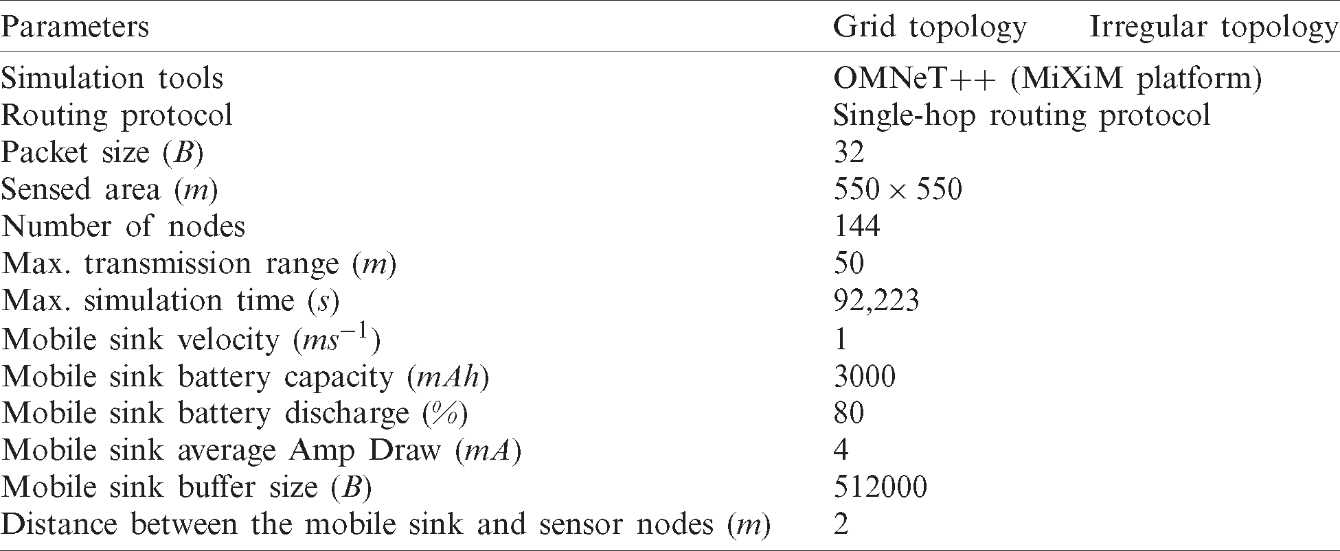
The proposed model is simulated using OMNeT++ [28]. The maximum simulation time can only be set to 92,223 s due to the restriction of the simulation tool. The simulation parameters are shown in Tab. 1.
Table 1: Simulation parameters
4.3 Simulation Result and Discussion for Irregular Topology
In the irregular topology, EPS-2 and EPS-3 are compared with several related strategies, namely RkM [26], RCTS [14], and NCTS [14]. The impacts of different strategies on packet lost percentage, average flight distance, and data delivery delay are investigated.
Fig. 6 illustrates the packet loss percentage for different strategies. It shows that the RkM has the highest value of packet loss percentage, which is 3.5% over its total packet collected. For EPS-2 and EPS-3, the packet loss percentages are 2.2% and 2.5% respectively. For RCTS and NCTS, the packet loss percentages are both closed to 1%. According to Tab. 2, 81% of the sensor nodes in RkM are assigned to an IP and 47% of the sensor nodes are connected to the same IP with three or more sensor nodes. Due to multiple connections are trying to be established between the mobile sink and the sensor nodes during limited contact duration, the channel is congested. Hence, the packet lost count in RkM is higher compared to the other mobility strategies. In EPS-2, at most two sensor nodes are registered to the same IP while in EPS-3, at most three sensor nodes are registered to the same IP. Therefore, the total packet loss of ESP-3 is higher than of ESP-2 because of the channel contention issue.

Figure 6: Packet loss % in irregular topology
Table 2: Percentage of sensor nodes formed one intermediate point
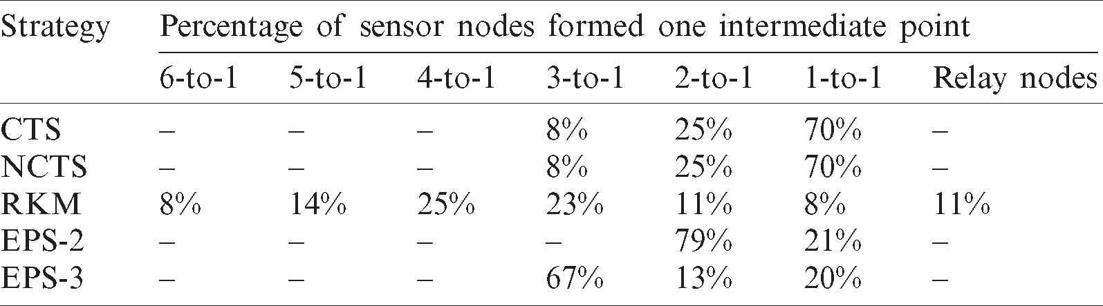
Fig. 6 shows that the packet lost percentages of RCTS and NCTS are the lowest among the mobility strategies. This is because according to Tab. 2, 70% of the sensor nodes in RCTS and NCTS do not share the IP with any other neighbors. Hence, the possibility of a packet loss to happen is lower compared to the other mobility strategies.
Fig. 6 proves that the fewer number of sensor nodes are registered to an IP results in a lower percentage of packet loss. However, more Ips that the mobile sink should visit and thus the fewer sensor nodes can be covered in each trip.
The average flight distance for these strategies is recorded as in Fig. 7. RkM uses the k-means clustering algorithm to obtain a set of potential positions of RP. Then the RP positions are utilized to obtain the flight trajectory by using Christofis’s heuristic [26]. EPS-2 and EPS-3 use IPS to obtain a set of IPs. After that, the IPs are utilized to obtain the flight trajectory by using GA.

Figure 7: Average flight distance per round trip in irregular topology
According to Fig. 7, RCTS and NCTS are having the highest average flight distance per round trip as compared to RkM, EPS-2, and EPS-3. In the irregular network topology, the density of sensor nodes in the sensed area is not equally distributed. Some areas in the sensed area may have none or fewer sensor nodes are allocated while some may have more. The flight trajectories that are applied in RCTS and NCTS cover every part of the sensed area. This includes the areas without any existence of a sensor node. However, areas without the allocation of sensor nodes are excluded from the flight trajectory that is applied in RkM, EPS-2, and EPS-3. Hence, the average flight distance per round trip for RCTS and NCTS are double of RkM, EPS-2, and EPS-3. This shows that the existence of the IPs reduces unnecessary flight distance during data collection.
Data delivery delay is one of the important factors to determine the efficiency of data collection in AGCWSN. The data delivery delay of the strategies is presented in Fig. 8 which shows that the data average delivery delay of RkM is 9360s, which is 120% higher than EPS-2. According to Fig. 7, the average flight distance for RkM is almost the same as EPS-2 and EPS-3. However, Tab. 2 also shows that 47% of the sensor nodes in RkM are registered to the same IP with three or more sensor nodes, which causes the channel contention issue. Besides that, the multi-hop routing protocol is applied in RkM. In the simulation, 11% of the sensor nodes relay the sensed data to the sensor nodes which are nearer to the IPs. The sensor nodes which act as relay nodes have to upload their own sensed data and their neighbors’ sensed data to the mobile sink within the limited contact duration. Within the limited contract duration between the mobile sink and the sensor nodes, a limited number of packets is received by the mobile sink. This causes a situation where the sensor nodes have packets that are yet to be uploaded to the mobile sink, but the mobile sink might have already left the communication range. Hence, the data delivery delay is high.
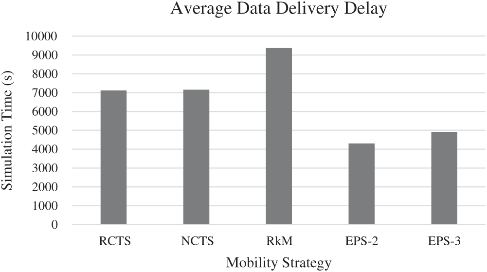
Figure 8: Average data delivery delay in irregular topology
The reason for RCTS and NCTS has a higher average data delivery delay, compared to EPS-2 and EPS-3, is because of their long flight distance which is shown in Fig. 7. The sensor nodes’ waiting time for the next approach of the mobile sink is longer, so the data delivery delay is higher. This shows that the data delivery delay is impacted by the number of sensor nodes which are connected to an IP and the flight distance taken by the mobile sink.
4.4 Simulation Result and Discussion for Grid Topology
To investigate the impact of IPs in the grid topology, EPS-2, TRS [23], RCTS [13], and NCTS [13] are simulated. The results are shown and the impacts of different strategies on packet lost percentages, average flight distance, and data delivery delay are discussed in this subsection. It should be noted that EPS-3 is not considered because in the grid topology being studied, it is not possible to find an IP to cover a group of 3 sensor nodes.
Fig. 9 shows the packet loss percentage for RCTS, NCTS, TRS, and EPS-2 in the grid topology. EPS-2 has the highest value of packet loss as shown in Fig. 9. This is due to only one sensor node establishes communication with the mobile sink in RCTS, NCTS, and TRS. But in EPS-2, two sensor nodes are trying to establish the connection with the mobile sink at the same transmission window. Therefore, the channel is congested which causes packet loss as shown in Tab. 3.

Figure 9: Packet loss % in grid topology
Table 3: Packet loss % in grid topology
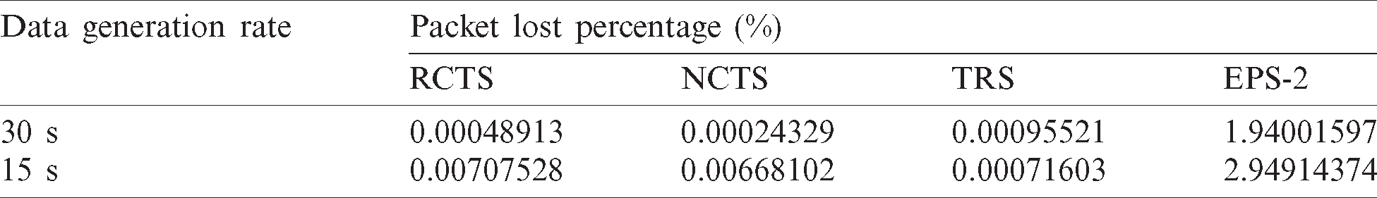
Fig. 10 presents the average flight trajectories of these strategies. The flight trajectories that are applied in RCTS and NCTS cover every part of the sensed area. This includes the areas without any existence of a sensor node. However, the areas without the allocation of sensor nodes are excluded from the flight trajectory which is applied in EPS-2. This is to preserve the mobile sink’s limited battery capacity during data collection. Hence, the average flight distance per round trip for RCTS and NCTS are 170% higher than EPS-2 as shown in Fig. 10.

Figure 10: Average flight distance per round trip in the grid topology
TRS is similar to RCTS and NCTS where the flight trajectory covers every part of the sensed area. However, according to Fig. 10, the average flight trajectory for TRS is 42% lower than RCTS and NCTS. This is because the mobile sink in TRS returns to the base station after collects data from two rows of the sensor nodes. However, the mobile sink in RCTS and NCTS only returns to the base station when its battery energy is running out. In the situation where the mobile sink in RCTS and NCTS stops the flight when it is visiting a sensor node which is located far away from the base station, the mobile sink spends a larger amount of time to return to the base station. The fully charged mobile sink is also required to spend a larger amount of time to reach the position where the previous mobile sink has stopped. This is the reason why the average flight distance for TRS is lesser than RCTS and NCTS.
Fig. 11 shows that the average data delivery delay for RCTS and NCTS are 120% higher than EPS-2. This is because EPS-2 has a shorter flight distance taken by the mobile sink during data collection as shown in Fig. 10. The average data delivery delay for all mobility strategies in the buffer full scenario is slightly higher than in the buffer non-full scenario. This is because in the buffer full scenario, the mobile sink returns to the base station due to the buffer is full. The remaining sensed data which is yet to be uploaded to the mobile sink will have to wait for the next mobile sink’s approach. Hence, the average data delivery delay is higher. Fig. 11 shows that the flight distance taken by the mobile sink greatly impacts the data delivery delay.

Figure 11: Average data delivery delay in the grid topology
In this paper, we have proposed an Energy-efficient Path-finding Strategy (EPS) in the Air-Ground Collaborative Wireless Sensor Network (AGCWSN) to improve the efficiency of data collection. The performance of the proposed strategy is compared with other existing strategies under the same simulation network model, parameters, and configuration. The simulation results show that EPSs outperform the other existing data collection strategies in terms of data delivery delay and utilization of the mobile sink’s battery capacity. It is observed that the proposed strategy has a higher packet loss percentage as compared to the strategies which do not have IP or RP involved. This is explained by the occurrence of channel contention issue when more than one sensor node is connected to the mobile sink during the same communication window. However, with the lower data delivery delay and better utilization of the mobile sink’s battery capacity, the proposed strategies still have much better performance as compared to the other strategies. For the future work, this study can be extended to multiple mobile sinks that operate simultaneously in the sensed area to further reduce data delivery latency. The data burst scenario can also be considered in the future simulation.
Acknowledgement: Thanks to our families and colleagues who supported us morally.
Funding Statement: The authors received no specific funding for this study.
Conflicts of Interest: The authors declare that they have no conflicts of interest to report regarding the present study.
1. D. Giri, S. Borah and R. Pradhan. (2018). “Approaches and measures to detect wormhole attach in wireless sensor networks: A survey,” In: R. Bera, S. Sarkar, S. Chakraborty, Advances in Communication, Devices and Networking. Lecture Notes in Electrical Engineering, Singapore: Springer, vol. 462. pp. 855–864. [Google Scholar]
2. H. Luo, K. Wu, R. Ruby, Y. Liang, Z. Guo et al. (2018). “Software-defined architectures and technologies for underwater wireless sensor networks: A survey,” IEEE Communications Surveys & Tutorials, vol. 20, no. 4, pp. 2855–2888. [Google Scholar]
3. K. Ghosh, S. Neogy, P. K. Das and M. Mehta. (2017). “Intrusion detection at international borders and large military barracks with multi-sink wireless sensor networks: An energy efficient solution,” Wireless Personal Communications, vol. 98, no. 1, pp. 1083–1101. [Google Scholar]
4. I. F. Akyildiz, W. Su, Y. Sankarasubramaniam and E. Cayirci. (2002). “Wireless sensor networks: A survey,” Computer Networks, vol. 38, no. 4, pp. 393–422. [Google Scholar]
5. M. Y. Kumar and A. Trivedi. (2014). “Performance improvement of clustered WSN by using multi-tier clustering,” in Handbook of Research on Progressive Trends in Wireless Communications and Networking, USA: IGI Global, pp. 365–388. [Google Scholar]
6. J. Zhou, Y. Liang, Q. Shen, X. Feng and Q. Pan. (2018). “A novel energy-efficient multi-sensor fusion wake-up control strategy based on a biomimetic infectious-immune mechanism for target tracking,” Sensors (Basel), vol. 18, no. 4, pp. 1255–1277. [Google Scholar]
7. S. Y. Liew, C. K. Tan, M. L. Gan and H. G. Goh. (2018). “A fast, adaptive, and energy-efficient data collection protocol in multi-channel-multi-path wireless sensor networks,” IEEE Computational Intelligence Magazine, IEEE, vol. 13, no. 1, pp. 30–40. [Google Scholar]
8. Z. Wadud, N. Javaid, M. A. Khan, N. Alrajeh and M. S. Alabed et al. (2017). “Lifetime maximization via hole alleviation in IoT enabling heterogeneous wireless sensor networks,” Sensors, vol. 17, no. 7, pp. 1677. [Google Scholar]
9. A. Khan, N. Javaid, A. Sher, R. A. Abbasi and Z. Ahmad et al. (2018). “Load balancing and collision avoidance using opportunitistic routing in wireless sensor networks,” in 2018 IEEE 32nd Int. Conf. on Advanced Information Networking and Applications, Krakow, pp. 236–243. [Google Scholar]
10. M. I. Khan, W. N. Gansterer and G. Haring. (2013). “Static vs. mobile sink: The influence of basic parameters on energy efficiency in wireless sensor networks,” Computer Communication, vol. 36, no. 9, pp. 965–978. [Google Scholar]
11. M. A. Rahman, S. Azad, A. T. Asyhari, M. Z. A. Bhuiyan and K. Anwar. (2018). “Collab-SAR: A collaborative avalanche search-and-rescue missions exploiting hostile alpine networks,” IEEE Access, vol. 6, pp. 42094–42107. [Google Scholar]
12. R. Dasgupta and A. Dasgupta. (2017). “A multiple-level method for miniziming data gathering latency in wireless sensor networks using mobile elements,” in Int. Conf. on Electrical, Computer and Communication Engineering, Cox’s Bazar, pp. 123–127. [Google Scholar]
13. L. Y. Tan, H. G. Goh, S. Y. Liew and S. K. Teoh. (2018). “Data store-and-delivery approach for air-ground collaborative wireless sensor network,” in 9th IEEE Control and System Graduate Research Colloquium, IEEE, Shah Alam, Malaysia, pp. 45–49, , 2018. [Google Scholar]
14. M. Assaf and M. Ndiaye. (2017). “Multi travelling salesman problem formulation,” 4th Int. Conf. on Industrial Engineering and Applications, vol. 2017, pp. 292–295. [Google Scholar]
15. A. A. Khan and H. Agrawal. (2016). “Optimization of delay of data delivery in wireless sensor network using genetic algorithm,” in 2016 Int. Conf. on Computation of Power, Energy Information and Communication, Chennai, pp. 159–164. [Google Scholar]
16. J. Lian, K. Naik and G. B. Agnew. (2006). “Data capacity improvement of wireless sensor networks using non-uniform sensor distribution,” International Journal of Distributed Sensor Networks, vol. 2, no. 2, pp. 121–145. [Google Scholar]
17. N. T. Hanh, P. L. Nguyen, P. T. Tuyen, H. T. Thanh and E. Kurniawan et al. (2018). “Node placement for target coverage and network connectivity in WSNs with multiple sinks,” in 15th IEEE Annual Consumer Communications and Networking Conference, Las Vegas, NV, pp. 1–6. [Google Scholar]
18. J. Chang and T. Shen. (2016). “An efficient tree-based power saving scheme for wireless sensor networks with mobile sink,” IEEE Sensors Journal, vol. 16, no. 20, pp. 7545–7557. [Google Scholar]
19. J. Wang, L. Zuo, Z. Zhang, F. Xia and J. Kim. (2013). “Mobility based data collection algorithm for wireless sensor networks,” in 2013 IEEE 9th Int. Conf. on Mobile Ad-hoc and Sensor Networks, Dalian, pp. 342–347. [Google Scholar]
20. Q. Tang, G. Tong, X. Wang, J. Shi and Y. Han. (2016). “An energy-efficient scheme for data collection in wireless sensor networks,” in 25th Wireless and Optical Communication Conf., PyeongChang, pp. 60–65. [Google Scholar]
21. P. Patil, U. Kulkarni and N. H. Ayachit. (2011). “Some issues in clustering algorithms for wireless sensor networks,” 2nd National Conf. on Computing, Communication and Sensor Network, vol. 4, no. 4, pp. 18–23. [Google Scholar]
22. M. Meghji and D. Habibi. (2011). “Transmission power control in multihop wireless sensor networks,” in Third Int. Conf. on Ubiquitous and Future Networks, Dalian, pp. 25–30, [Google Scholar]
23. P. Mathur, R. H. Nielsen, N. R. Prasad and R. Prasad. (2016). “Data collection using miniature aerial vehicles in wireless sensor networks,” IET Wireless Sensor Systems, vol. 6, no. 1, pp. 17–25. [Google Scholar]
24. J. Valente, D. Sanz, A. Barrientos, J. D. Cerro, A. Ribeiro et al. (2011). “An air-ground wireless sensor network for crop monitoring,” Sensors, vol. 11, no. 6, pp. 6088–6108. [Google Scholar]
25. A. Bujari, C. T. Calafate, J. Cano, P. Manzoni, C. E. Palazzi et al. (2017). “Flying ad-hoc network application scenarios and mobility models,” International Journal of Distributed Sensor Networks, vol. 13, no. 10, pp. 155014771773819. [Google Scholar]
26. A. Kaswan, K. Nitesh and P. K. Jana. (2017). “Energy efficient path selection for mobile sink and data gathering in wireless sensor networks,” International Journal of Electronics and Communications, vol. 73, pp. 110–118. [Google Scholar]
27. A. Jaradat, B. Matalkeh and W. Diabat. (2019). “Solving travelling salesman problem using firefly algorithm and k-means clustering,” in IEEE Jordan Int. Joint Conf. on Electrical Engineering and Information Technology, Amman, Jordan, pp. 586–589. [Google Scholar]
28. A. Varga. (2010). “OMNeT++,” In: K. Wehrle, M. Gunes, J. Gross, Modeling and Tools for Network Simulation, vol. 3. Berlin, Heidelberg: Springer, pp. 35–59. [Google Scholar]
 | This work is licensed under a Creative Commons Attribution 4.0 International License, which permits unrestricted use, distribution, and reproduction in any medium, provided the original work is properly cited. |