DOI:10.32604/cmc.2021.015294
| Computers, Materials & Continua DOI:10.32604/cmc.2021.015294 | |
| Article |
Feasibility-Guided Constraint-Handling Techniques for Engineering Optimization Problems
1Institute of Numerical Sciences, Kohat University of Science & Technology, Kohat, Pakistan
2Department of Economics, Abbottabad University of Science & Technology, Abbottabad, Pakistan
3Institute of Computing, Kohat University of Science & Technology, Kohat, Pakistan
4Faculty of Applied Studies, King Abdulaziz University, Jeddah, Saudi Arabia
5Jinnah College for Women, University of Peshawar, Peshawar, Pakistan
6Department of Physics, Kohat University of Science & Technology, Kohat, Pakistan
*Corresponding Author: Muhammad Asif Jan. Email: majan.math@gmail.com; majan@kust.edu.pk
Received: 14 November 2020; Accepted: 02 January 2021
Abstract: The particle swarm optimization (PSO) algorithm is an established nature-inspired population-based meta-heuristic that replicates the synchronizing movements of birds and fish. PSO is essentially an unconstrained algorithm and requires constraint handling techniques (CHTs) to solve constrained optimization problems (COPs). For this purpose, we integrate two CHTs, the superiority of feasibility (SF) and the violation constraint-handling (VCH), with a PSO. These CHTs distinguish feasible solutions from infeasible ones. Moreover, in SF, the selection of infeasible solutions is based on their degree of constraint violations, whereas in VCH, the number of constraint violations by an infeasible solution is of more importance. Therefore, a PSO is adapted for constrained optimization, yielding two constrained variants, denoted SF-PSO and VCH-PSO. Both SF-PSO and VCH-PSO are evaluated with respect to five engineering problems: the Himmelblau’s nonlinear optimization, the welded beam design, the spring design, the pressure vessel design, and the three-bar truss design. The simulation results show that both algorithms are consistent in terms of their solutions to these problems, including their different available versions. Comparison of the SF-PSO and the VCH-PSO with other existing algorithms on the tested problems shows that the proposed algorithms have lower computational cost in terms of the number of function evaluations used. We also report our disagreement with some unjust comparisons made by other researchers regarding the tested problems and their different variants.
Keywords: Constrained evolutionary optimization; constraint handling techniques; superiority of feasibility; violation constraint-handling technique; swarm based evolutionary algorithms; particle swarm optimization; engineering optimization problems
Optimization can be simply defined as the process of searching for the best outcome. The process of optimization is not new to human beings; they have been applying it since the dawn of time. Owing to its role in solving real-world problems, optimization is imperative for research in applied mathematics. With the advent of digital computing machines in the early 1950s, population-based stochastic algorithms started to develop, paving the way for solutions to complex optimization problems that were previously considered to be unsolvable [1]. In particular, during the past five decades, optimization has emerged as a new branch of computational mathematics. Optimization can be categorized into two main sub-branches: unconstrained optimization and constrained optimization. In an unconstrained optimization, each objective or cost function is optimized without any constraint, whereas in a constrained optimization, the objective or cost function is optimized subject to certain constraints. As almost all real-world problems can be modeled as constrained optimization problems (COPs), algorithms designed for unconstrained optimization are often hybridized with CHTs to solve these problems.
Without loss of generality, in the minimization sense, a COP can be defined as follows [2]:
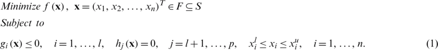
In problem (1),  is called the objective function, which is to be minimized. In the case of maximization,
  is multiplied with a negative sign. The n-dimensional vector
  is called the decision variables vector. There are l inequality-type and p − l equality-type constraints.
  and
and  are the lower and upper bounds for the component xi of the decision variable vector
  . These bounds define the search space S. Solutions that meet all constraints of problem (1) are called feasible solutions. If F is the feasible region containing all feasible solutions, then
  . On the other hand, solutions that violate any of the constraints of problem (1) are called infeasible solutions, and the region of all such solutions is called the infeasible region.
Nature-inspired algorithms (NIAs), as the name suggests, are inspired by successful biological and/or physical systems in nature [3]. NIAs are population-based meta-heuristics and have two major subdivisions: evolutionary algorithms (EAs) and swarm intelligence (SI)-based algorithms. EAs are optimization techniques that work on Darwin’s principle of “survival of the fittest” [4], whereas the main theme of SI-based algorithms is communication among members of a swarm. Through this communication, they learn from the experience of other members of the swarm, and the swarm reaches a level of intelligence that no individual could attain. Designing SI-based algorithms is a relatively new research area in the field of NIAs. Important SI-based algorithms include ant colony optimization [5], the bat algorithm (BA) [5], firefly algorithm (FA) [5], and particle swarm optimization (PSO) [6].
PSO was developed by Kennedy and Eberhart in 1995. Owing to its ease of implementation, PSO is one of the most widely used SI-based algorithms. In the PSO algorithm, an initial population of particles (swarm members) is generated randomly in a given search space. Each particle is assigned a velocity. In subsequent iterations, the velocity of each particle is updated using appropriate formulae. This updated velocity is then used to update the position of the particle. This process of updating velocities and then positions is repeated until some stopping criteria are fulfilled. To deal with constrained problems, PSO, like other EAs and SI-based algorithms, needs modification in the sense that some CHT must be incorporated into its framework. Several such modifications for single- and multi-objective constrained optimization are detailed in [7–15].
Any parameter-free CHT is preferred over the commonly used penalty function approach for constraint handling provided it gives competitive results. The superiority of feasibility (SF) [16] approach is one such CHT. In a penalty function approach, if competing solutions are feasible, then selection among them for the next generation is based on their objective functions’ values. However, if competing solutions are infeasible, then their objective functions’ values are augmented with penalty terms. The SF technique is different in that if the competing solutions are infeasible, their functions’ values are not important; instead, their degrees of infeasibility are used in their ranking.
In [17], a new CHT, violation constraint-handling (VCH), was introduced, using the number of constraint violations as a decisive factor. The authors developed VCH-GA by combining VCH with a genetic algorithm (GA), and obtained striking results for some engineering problems. This technique is similar to SF, with some modifications towards the end. In this technique, candidates with fewer constraint violations are preferred over candidates with more constraint violations. In this work, we integrate SF and VCH into the PSO framework to handle the constraints of problem (1), thereby adapting PSO for constrained optimization and designing two constrained versions of PSO, denoted SF-PSO and VCH-PSO.
The remainder of the paper is organized as follows. Section 2 contains a brief literature review pertaining to PSO and some constrained versions of PSO. Section 3 presents a brief introduction of the two CHTs and details of proposed algorithms. Section 4 presents and discusses experimental results. A short summary of the work and plans for the future are given in the concluding Section 5.
In this section, we first describe PSO and a number of its improved variants. Then, a number of promising constrained algorithms employing PSO as a base algorithm are discussed.
PSO is among the most popular algorithms in the field of optimization. It has been widely used in various applications including in engineering and industry. PSO was inspired by the navigation patterns and synchronized movements of bird flocks. PSO was developed in 1995 for unconstrained optimization problems. Over the years, various versions of PSO have been developed. Owing to its ease of implementation, PSO is among the most widely used SI-based algorithms. However, PSO differs from EAs, as it assumes that a member of the swarm never dies but rather flies from one place to another in a given search space. In the PSO algorithm, an initial population of particles (swarm members) is generated randomly in a given search space. Each particle is assigned a velocity, which can initially be set to zero or generated randomly [18]. In subsequent iterations, the velocity of the ith particle at generation t + 1,  , is updated using the following equation [19]:

where  is the current velocity,
  is the current position,
  is the best particle in the linage of the ith particle,
  is the best particle of the entire population so far, and
  and
and  are randomly generated vectors with components lying between 0 and 1 that give a stochastic nature to the algorithm. In Eq. (2), the first term on the right-hand side is the velocity of the particle in the previous generation and is termed the inertia component. One purpose of this component is to avoid any abrupt change in the direction of the particle. The second term is based on the personal experiences of the particle and is called the cognitive component, while the third term is based on the experiences of the whole swarm and is called the social component. In the initial version of PSO, r1 and r2 were randomly generated numbers, but the authors soon replaced them with randomly generated vectors. Parameters c1 and c2 are learning parameters used to balance the local and global search. In the initial version of PSO, these two parameters were set to 2. The role of these two parameters is very important, as they control the explorative and exploitative capabilities of the algorithm. A higher value of c1 means a higher rate of exploration, and a higher value of c2 means a higher rate of exploitation. In initial versions, these parameters were kept constant, but intuition suggests a higher c1 value for the initial iterations to enable maximum exploration of the search space, and a higher c2 value for the last iterations to exploit the regions with a possible solution (global optima). This intuitive idea is now an essential part of modern versions of PSO. In [20], the idea of time-varying acceleration coefficients was applied. In Eq. (2), a larger value of c1 and a smaller value of c2 in the initial stages ensure exploration of the whole search space. Gradual reduction of the weight of the cognitive component through c1 and an increase in the weight of the social component through c2 facilitate global convergence. Mathematically, the two coefficients of the cognitive and social components are updated as follows [20]:


where c1i and c1f are lower and upper bounds for the cognitive component, while c2i and c2f are lower and upper bounds for the social component. In [20], after much experimentation, the authors proposed reducing c1 from 2.5 to 0.5 and increasing c2 from 0.5 to 2.5 for better performance. In [21], Vmax was introduced. This parameter keeps the newly generated particles in a given search space and controls the search steps.
As we can see from the inertia component of Eq. (2), the velocity of a particle in the previous iteration is fully utilized in updating its velocity for the next iteration. However, this may not always be the preferred choice. Sometimes, we may wish to use only a fraction of the velocity. More precisely, we may wish to use a larger fraction of the velocity in the initial iterations to explore the whole search space, whereas in later iterations, a smaller fraction of the previous velocity is preferable to exploit the regions with higher probabilities of having solutions. This can be accomplished using a new parameter  , termed the inertia weight [21]. To control the weight of the velocity at various stages, the following equation for updating the velocity contains an inertia factor
  :
:

When first introduced, the inertia weight was kept constant, but various researchers soon experimented with changing the value of the parameter  . In [21], the authors used a linearly changing inertia weight and noted a significant improvement in the performance of their algorithm as a result. The formula for updating
  is as follows [21]:

where  and
and  are the lower and upper bounds of the inertia weight,
  is the total number of iterations, and It is the current iteration number. The authors observed through experiments that the algorithms performed well when 0.4 and 0.9 were used as lower and upper bounds for
  .
.
The parameter  given by Eq. (6) does well in static problems but not so well in dynamic systems. Another formula for updating
  randomly was introduced in [21]. This
  , as given by the following equation, improved the performance of algorithms for dynamic systems [21]:

The velocity given by Eqs. (2) or (5) is used to update the position of the ith particle in generation t + 1,  , as follows [19]:

As far as the population size of the swarm is concerned, there is no significant difference in the results when the population size is varied [21]. Conversely, larger the population size, higher the computational costs, which is generally not desirable, particularly in engineering problems. Although in [22] the concept of a small population (five particles) with a re-initialization option was adopted to maintain diversity, a normal range of 20 to 60 particles was used in most of the existing literature.
Owing to the fast converging capability of PSO, various researchers have integrated it with CHTs for solving COPs. Some of the prominent works using PSO as a base algorithm are described in the following sections.
In FS-PSO [23], the preservation of feasible solutions (FS) method is incorporated into PSO to deal with constraints in COPs. This method requires a feasible initial population, and the feasibility of solutions is maintained throughout subsequent generations. As there exists no infeasible solution, the entire search process will be confined to the feasible region. Hence, selection of the winner is solely based on the objective function value. This method seems simple in the sense that it considers feasible solutions only, and there is no question of constraint violations. However, in some problems, the feasible region is small compared with the given search space. Also, there are problems in which it is difficult to generate a single feasible solution, let alone a whole population. In [22], the authors could not find a single feasible solution among one million randomly generated solutions for some problems. Thus, the idea of having a feasible population at the start of each problem is almost impractical. In cases where we have the entire feasible population at the start of the problem, it is not confirmed that there will be a whole feasible population at the next generation unless the search space is convex.
In HPSO [24], PSO is hybridized with SF to solve COPs. This rule is quite strict in the case of infeasible solutions, which are radially discarded in comparison with feasible solutions, leading to premature convergence. The authors avoided premature convergence by using simulated annealing (SA). The global best is perturbed by SA to escape local optima.
In HPSO, the personal best solution,  , is selected per the SF rule, whereas SA is employed during selection of the generational best solution,
  . Furthermore, the authors kept the number of generations quite low at 300 in their experiments, but they used a population of 250 particles, which is quite large in comparison with those used in other contemporary PSO algorithms.
The authors of SR-PSO incorporated stochastic ranking (SR) into PSO to develop a hybrid algorithm for COPs. Although SR is a popular CHT that works quite well in most cases, there remains a user-defined parameter Pf in this technique. In this technique, if particles are feasible or a randomly generated number, rand, is less than Pf, then particles are ranked per their objective function values; otherwise, they are ranked per their constraint violations. As parameters are always hard to fine-tune, if Pf is too high, most of the infeasible solutions will be ranked per objective function values, and the role of constraint violations will be minimal. Of course, this is not a good idea. On the other hand, if Pf is kept low, most of the infeasible solutions will be ranked per constraint violations, and the role of objective function values will be minimal. Again, this is not a good idea. A balance between the two is preferable for any algorithm. Algorithms based on SR cannot be termed as properly guided, as many of the outcomes rely on Pf and rand with no or very limited use of previous knowledge. Another drawback is that the algorithm does not implement PSO in a real sense, as particles never die in PSO, whereas in SR-PSO some of the particles are discarded. PSO does not have an explicit selection. Also, in SR-PSO, generating npop particles from  particles is a form of crossover.
In [25], the authors used a combination of an epsilon constraint method and PSO to develop  -PSO, a technique based on
  -level comparison. In [26], the authors integrated PSO with an
  -constraint-handling method based on
  -level comparison. According to [25], the two techniques are theoretically equivalent. A satisfaction level
  is defined for constraints of the problem. For feasible solutions,
  . For
. For  , if
, if  and
and  are less than
  , objective function values are used for ranking particles, otherwise their satisfaction levels
  and
and  are used. Equality constraints can be coped with very easily by relaxing constraints at early stages and then tightening them gradually. Both techniques closely resemble SR.
In [27], a non-stationary multi-stage assignment penalty function was combined with PSO to solve COPs. In this approach, the actual objective function is augmented with a penalty term, based on constraint violations, to form a fitness function. This fitness function is then used for ranking particles. By contrast, in our proposed technique, no new function is formed. For ranking particles, objective function values and constraint violations are considered separately, one at a time. The newly developed algorithm achieved competitive results on the CEC 2006 test functions suite.
In [28], a newly proposed self-adaptive strategy was added to the standard PSO 2011 algorithm, resulting in a modified PSO algorithm, SASPSO 2011. Furthermore, for population diversity, an adaptive relaxation method is combined with a feasibility-based rule to handle constraints and evaluate solutions in the suggested framework. In SASPSO 2011, the number of parameters is increased, although they are adjusted adaptively. By contrast, our proposed technique VCH-PSO uses a very basic version of PSO to keep the number of parameters low. Another main difference is that VCH-PSO considers the actual feasible region of the problem, whereas in [28], similar to the  and
and  techniques, constraints are initially relaxed to consider larger regions as feasible. Furthermore, unlike feasibility-based rules, VCH-PSO mainly focuses on the number of constraint violations rather than their degree. The performance of SASPSO 2011 was evaluated and compared on four benchmark and two engineering problems against six PSO variants and some well-known algorithms. The authors claimed promising performance of SASPSO 2011 versus competitors. The comparison of simulation results of VCH-PSO and SASPSO 2011 on the two engineering problems, spring design and three-bar truss design, can be seen in Tabs. 6 and 9.
In this section, first we briefly describe the two CHTs that were used to adapt PSO for constrained optimization. Then, the two adapted algorithms, SF-PSO and VCH-PSO, are detailed.
3.1 Superiority of Feasibility
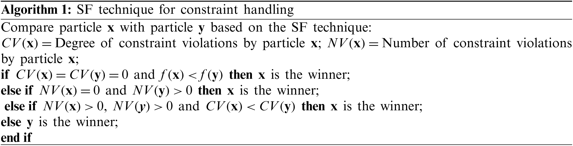
Any parameter-free CHT will be preferred over a penalty function approach if it gives competitive results. The SF technique is one such CHT. In a penalty function approach, if competing solutions are feasible, the selection is based on objective function values; if competing solutions are infeasible, objective function values are augmented with a penalty term. The SF technique is different in the sense that if the competing solutions are infeasible, their objective function values are no longer important, and their degrees of infeasibility are considered for their ranking. Furthermore, the SF technique is a combination of two different categories. On the one hand, it separates feasible solutions from infeasible ones; on the other hand, it penalizes infeasible solutions. If competing solutions are infeasible, their constraint violations will be used to augment the objective function value of the worst feasible solution, not the competing solution’s own objective function value. This fitness function is constructed as follows:

where  is the maximum objective function value (worst in the minimization sense) calculated from feasible solutions. At any stage of the algorithm, if there is no feasible solution, then
  is taken to be zero. There are following three cases for the selection of winner in the SF technique.
1. Between two feasible solutions, winner will be the one with the lower objective function value.
2. Between a feasible and an infeasible solution, a feasible solution will always be preferred over an infeasible one.
3. Between two infeasible solutions, the winner will be the one with the lesser degree of constraint violations.
The pseudo-code for selection in the SF technique is given in Algorithm 1.
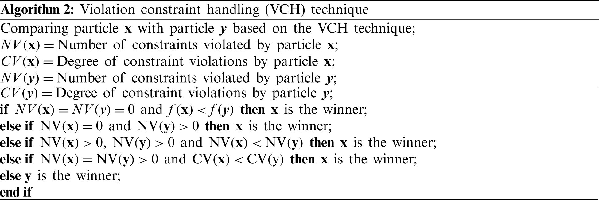
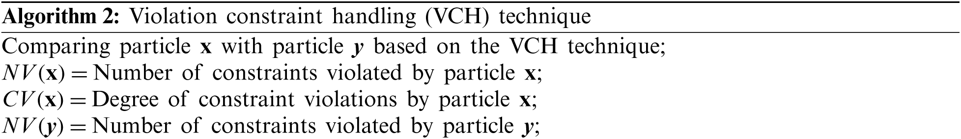
In VCH technique, the number of constraint violations was used as a preferred CHT. Here, selection of the winner is made in such a way that if the two competitors are infeasible, the winner will be pushed towards the feasible region. If the competitors are feasible, the quality of the solution will be improved. In any CHT, the criteria for selection of a winner among the infeasible competitors is mainly based on either their distance from the feasible region or the degrees of their constraint violations. In VCH, it is the number of constraint violations that decides the fate of infeasible competitors. VCH is a CHT that is based on the principle of “survival of the fittest.” Fortune cannot favor a solution that is not fit. On the other hand, techniques such as SR have a space for the survival of the luckiest. A solution can go to the next generation by chance even though it may be the worst with respect to the degree of constraint violations. In SR, if for a user-defined parameter Pf, we have  and both competitors are infeasible, a competitor with lower function value and a high degree of constraint violations will find space in the next generation. As VCH is hard on infeasible solutions, one may think of the diversity of the population. However, that is not an issue, because diversity in a population can be maintained through the randomness involved in the PSO algorithm. Nor is the burden of penalty parameter tuning an issue, as VCH is a parameter-free CHT. There are following four cases for the selection of a winner in VCH.
1. Between two feasible solutions, the winner will be the one with the lower objective function value.
2. Between a feasible and an infeasible solution, a feasible solution will always be preferred over an infeasible one.
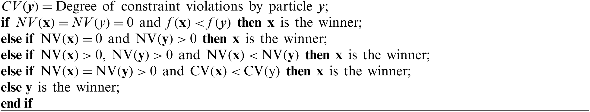
3. Between two infeasible solutions, the winner will be the one with the smaller number of constraint violations.
4. Between two infeasible solutions having the same number of constraint violations, the winner will be the one with lesser degree of constraint violations.

The pseudo-code of VCH is given in Algorithm 2.
:
3.3 Adapted Algorithms: VCH-PSO and SF-PSO
PSO in its original version, like the majority of other meta-heuristics, was developed for unconstrained problems. To deal with constrained problems, the PSO algorithm needs modification in the sense that some CHT must be incorporated into its framework. Two adapted algorithms, VCH-PSO and SF-PSO, for problem (1) are developed in this work through integrating VCH and SF into the PSO framework. The motive behind this hybridization was to combine the robustness and quick convergence of PSO with the simplicity and effectiveness of VCH and SF. Integrating these CHTs does not change the original objective function of the given problem, whereas the penalty function approach does. The SF technique was already integrated with PSO, but the authors also used SA to perturb  . The reason for this perturbation was to avoid local optima. In this work, we will show that our proposed algorithm SF-PSO can work well without SA.
Although the SF technique is sometimes placed into the category of CHTs that separate feasible solutions from infeasible solutions, it does not do so in a true sense. Rather, it adds the amount of infeasibility to the objective function value of the worst feasible solution, such that infeasible solutions are penalized without giving weight to the penalty term. Thus, the SF technique can be referred as a parameter-free penalty function approach. SF-PSO differs from the SF technique in the sense that in the case of infeasible solutions, the objective function value of the worst feasible solution is not added to form the new fitness function. For infeasible competitors, the degree of constraint violations is the sole decisive factor in SF-PSO.
In VCH-PSO, the decision is solely based on the number of constraint violations when comparing infeasible solutions. If the numbers of constraint violations for two competitors are equal, then the degree of violation will be the basis for selection of the winner. The focus of this research was to solve COPs of type (1). In our proposed algorithms, equality constraints present in any problem are transformed into inequalities as follows:

where  is a small positive number. In our experiments, it is taken as 1e −4, which is the standard that is normally used in the literature. The pseudo-code of VCH-PSO is given in Algorithm 3. The flowchart of VCH-PSO is shown in Fig. 1. The pseudo-code of SF-PSO is almost the same as that of VCH-PSO; the only differences are in the update criteria for
  and
and  . In SF-PSO, the update criteria for
  and
and  are based on Algorithm 1.

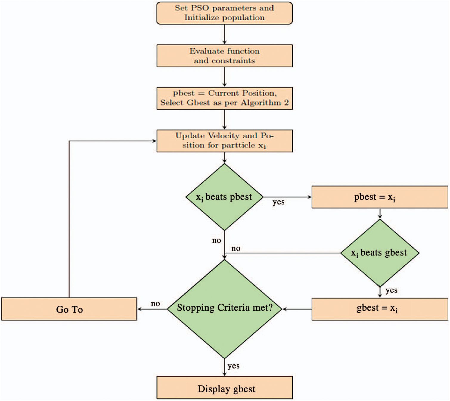
Figure 1: Flowchart of VCH-PSO algorithm
4 Simulation Results and Discussion
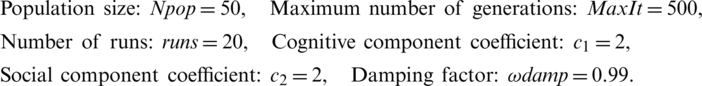
In order to evaluate the performance of the proposed algorithms, five engineering problems were selected from the available literature. All these problems were constrained and non-linear. As these problems had already been attempted by various researchers, a comparative study was used to help evaluate the performance of the proposed algorithms. The results were compiled from 20 independent runs of each algorithm on each problem. The PC configuration and parameter settings used were as follows.
The system used for the simulations ran Windows 10 with 8 GB RAM and a Core m3 1.00 GHz processor. All experiments were performed in the MATLAB R2013a environment.
In this section, the experimental results are discussed for the selected engineering problems. It can be noted from the comparison tables that different researchers used different numbers of function evaluations (NFEs) to reach the optimum, which makes comparison hard and the derived conclusions weak and non-affirmative.
4.3.1 Himmelblau’s Nonlinear Optimization Problem
This nonlinear optimization problem was proposed by Himmelblau in 1972 [29]. It has been widely used as a yardstick to check the performance of algorithms devised for nonlinear COPs. The problem was also included in the CEC 2006 suite [30]. The problem has five decision variables, six nonlinear inequality constraints, and ten boundary conditions. The optimal solution of this problem, as given in a special session on CEC 2006 by [30], is −30665.53 with decision variable vector [78, 33, 29.99, 45, 36.7758].
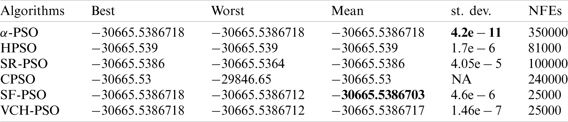
Tab. 1 shows results of VCH-PSO, SF-PSO, and some other algorithms for the problem. The results of other algorithms have been taken from the respective papers, and the last column of this table indicates the NFEs taken by each individual algorithm to reach the optimal solution. As can be seen in this column, both our algorithms, VCH-PSO and SF-PSO, achieved the global optimum with minimum NFEs = 25000. The small standard deviation (st. dev.) values achieved by our algorithms with less effort indicate the consistency of both algorithms.
Table 1: Comparison of proposed and other algorithms on Himmelblau’s nonlinear problem (version 1)
Some researchers have claimed far better results than the ones as mentioned in Tab. 1; for some examples, see [17,25,31]. However, they made a slight change in the first constraint of the problem to achieve their results and unfairly compared their results with those of researchers who attempted a different version of the problem. In this work, both versions of the problem have been attempted.
Tab. 2 shows results for another version (version 2). In this version, the first constraint of the problem is replaced by the following function:

Table 2: Comparison of proposed and other algorithms on Himmelblau’s nonlinear problem (version 2)
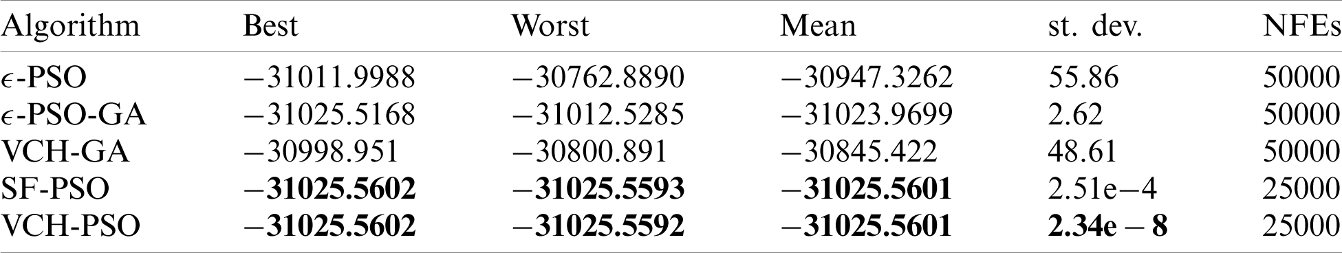
This change in the problem definition has greatly affected the results. The results for this second version attained by our algorithms VCH-PSO and SF-PSO are compared with those of  -PSO,
-PSO,  -PSO-GA, and VCH-GA.
Tab. 2 shows some interesting results. SF-PSO and VCH-PSO outperformed the above-mentioned algorithms in all respects using NFEs = 25000. Even the worst values attained by SF-PSO and VCH-PSO were better than the best of the rest. The design variables for the best solution by VCH-PSO were x1 = 78.000000000009393, x2 = 33.000000001832397, x3 = 27.070997106372257, x4 = 44.999999999998280, x5 = 44.969242546562349. The small st. dev. values for our both algorithms indicate their strength.
4.3.2 Welded Beam Design Problem
This problem was originally proposed by Rao in 1996 [32] and has been used as a benchmark problem to evaluate algorithms. The problem is to minimize the cost of constructing a welded beam with constraints on the sheer stress in the weld ( ), bending stress in the beam (
 ), buckling load on the bar (Pc), and end deflection of the beam (
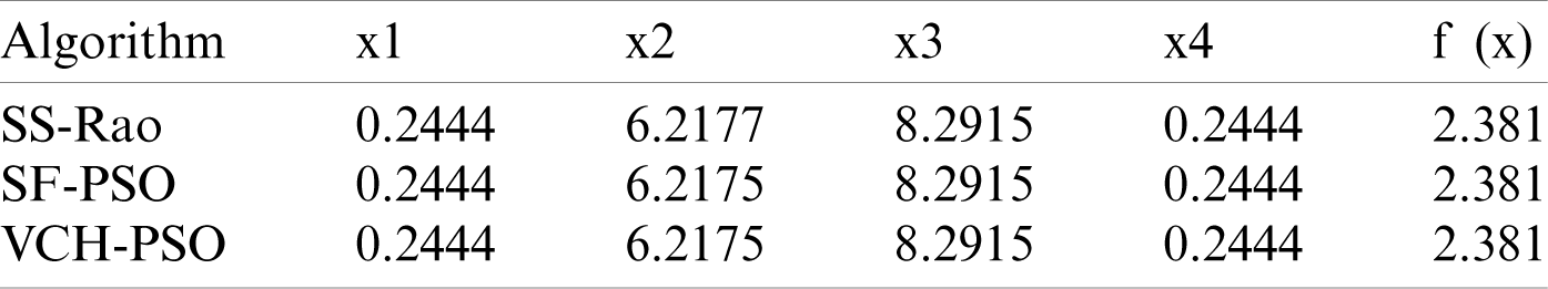
 ), as well as side constraints. Four decision variables represent the length of the beam, thickness of the beam, length of the weld, and thickness of the weld. The optimal solution, reported by Rao, is 2.3810 with solution vector [0.2444, 6.2177, 8.2915, 0.2444]. This problem is reported differently in the literature. The number of constraints used and various terms involved in the constraints differ among different researchers [17,19,33,34]. This difference in definition greatly affects the results, as evidenced by the wide differences in some comparison tables by various researchers. Three different versions of the problem were used here to test the proposed algorithms. Four different comparison tables have been constructed, keeping in mind the different versions of the problem.
Tab. 3 gives a comparison of the best solutions obtained by SS-Rao, SF-PSO, and VCH-PSO. VCH-PSO, and SF-PSO achieved the same results as SS-Rao.
Table 3: Comparison of proposed and other algorithms on welded beam problem (version 1)
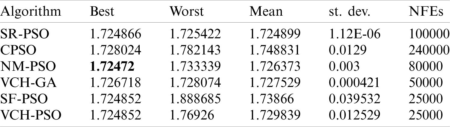
Tab. 4 gives a comparative analysis of VCH-PSO and SF-PSO with some contemporary well-known algorithms. The results indicate that the proposed algorithms, VCH-PSO and SF-PSO, are quite effective at attaining the minimum using NFEs = 25000. The small st. dev. values were also an indicator of our algorithms’ consistency. However, for this version of the problem, NM-PSO was best at attaining the minimum value when using NFEs = 80000. The welded beam problem has another version defined in BWOA [33], which is different from the version described by [32] and the majority of researchers. It will be referred to as version 3.
Table 4: Comparison of proposed and other algorithms on welded beam problem (version 2)
Tab. 5 gives a comparison of the best solutions obtained by PSO-GA, BWOA, VCH-PSO, and SF-PSO for the third version of the problem. Again, VCH-PSO and SF-PSO performed better than BWOA. Yet another version of the problem, different from the above three, is given in [16,34], where five constraints instead of seven are mentioned.
Table 5: Comparison of proposed and other algorithms on welded beam problem (version 3)

The spring design problem was first proposed by Arora in 1989 [35]. The problem is to minimize the weight of a tension spring, where the minimum deflection, sheer stress, surge frequency, and outside diameter are subject to constraints. The problem has three decision variables: x1 is the diameter of the wire from which the spring is made, x2 is the diameter of the spring, and x3 is the number of active coils. Although some researchers have considered the third variable, x3, as an integer, the majority have treated all three variables as continuous.
Optimal solutions obtained by VCH-PSO, SF-PSO, and some other contemporary algorithms are listed in Tab. 6. The last column of this table shows the NFEs taken by each individual algorithm.
Table 6: Comparison of proposed and other algorithms on spring design problem

This table indicates that VCH-PSO and SF-PSO attained the same best results with NFEs = 25000 as a recent algorithm, ETEO [36], with NFEs = 8100. Although the mean value of 20 runs for our proposed algorithms was slightly higher than those of competitors, the small st. dev. values indicate their consistency.
4.3.4 Design of a Pressure Vessel
This problem is based on the minimization of the cost of manufacturing a vessel that can be used to store air. Four decision variables are used to represent the thickness of the vessel, thickness of the head, internal radius, and length of the cylindrical section of the vessel. The problem was proposed by Sandgren in 1988 [37]. Various researchers have attempted the problem. There are two issues with the problem. Different researchers have defined the objective function differently [17,19,33]. Some researchers have treated the first two variables as discrete (being multiples of 0.0625) and the other two as continuous [17], while others have treated all the variables as continuous [33]. In the literature, there exist some comparison tables, in which the optima obtained differ by wide margins. At first glance, some researchers seem to have developed superior algorithms, but our study reveals some unfair comparisons. These wide differences are often due to differences in the definition of the problem and not in the performance of the individual algorithm. In this work, the VCH-PSO and SF-PSO algorithms are applied to models, treating all variables as continuous. Although four different versions of the problem have been noted, only two have been attempted. Comparison is made with only those researchers who used the same model of the problem as proposed in [37].
Tab. 7 lists simulation results obtained with VCH-PSO, SF-PSO, and some other algorithms. Although SF-PSO achieved the minimum with NFEs = 25000 of all the algorithms, the high average and st. dev. values for our proposed algorithms reveal the weak performance of VCH-PSO and SF-PSO for this version of the problem.
Table 7: Comparison of proposed and other algorithms on pressure vessel design problem (version 1)

Tab. 8 lists data for version 2 of the problem. This table gives a comparison of the best solutions obtained by the BWOA, VCH-PSO, and SF-PSO algorithms, showing that VCH-PSO and SF-PSO surpass the BWOA algorithm in terms of the “best” value.
Table 8: Comparison of proposed and other algorithms on pressure vessel design problem (version 2)

Kannan and Kramer designed this problem in 1994 [38]. The problem is to minimize the volume of a three-bar truss structure, which is subjected to some stress constraints. The design must sustain a certain load without elastic failure.
Tab. 9 shows a comparison of the proposed algorithms with BA [38], SR-PSO, CSA [39], SRIFA [40], and ETEO. Although ETEO attained the best result with only 600 NFEs, our algorithm VCH-PSO with NFEs = 25000 achieved the same best result as CSA, SRIFA, and ETEO. SF-PSO also achieved a best result close to the known solution. However, the results for CSA with NFEs = 25000 were better in terms of mean, st. dev., and NFEs.
Table 9: Comparison of proposed and other algorithms on three-bar truss problem

In this work, two constrained variants of PSO, SF-PSO and VCH-PSO, are proposed. The performance of both algorithms has been evaluated on five engineering problems. Two issues regarding these problems have been identified through this work. First, different versions of the problems exist. Himmelblau’s nonlinear problem has two versions that differ in the constraints involved. The welded beam problem has three versions, which vary in constraints’ definitions and the terms involved in constraints. The pressure vessel problem has four different versions, which differ in the definition of the objective function. The second issue is regarding the bounds for decision variables. Various researchers have used different bounds. This greatly affects the results, as changing the bounds means changing the search space.
For the first version of Himmelblau’s problem, both algorithms attained the optima mentioned in the literature. For the second version of the problem, the algorithms obtained better results than some well-known recent algorithms. Three different versions of the welded beam problem were tried: In the first two versions, our algorithms produced competitive results, while for the third version, our results were better than those of the competitors. For the spring design problem, our algorithms performed better than some state-of-the-art algorithms. In the first version of the pressure vessel design problem, VCH-PSO and SF-PSO gave high mean and st. dev. values, indicating their weak performance. However, for the second version, Chen’s algorithm BWOA was surpassed by a wide margin. For the three-bar truss problem, VCH-PSO gave better results but with a narrow margin. These results are encouraging, as VCH-PSO attained the optimum with a 100% feasibility rate. The low st. dev. values in most cases indicate the consistent performance of the proposed algorithms. The experimental results show no marked difference between the proposed algorithms. It may also be noted that our proposed algorithms achieved results better than or comparable with those of competing algorithms on most of the tested problems, with fewer NFEs used.
In future, the SF and VCH techniques will be implemented in other SI-based algorithms such as the FA and BA to adapt them for constrained optimization.
Funding Statement: The authors thank the Higher Education Commission, Pakistan, for supporting this research under the project NRPU-8925 (M.A.J. and H.U.K.), https://www.hec.gov.pk/.
Conflicts of Interest: The authors declare that they have no conflicts of interest to report regarding the present study.
1. A. Antoniou and W. S. Lu. (2007). Practical Optimization: Algorithms and Engineering Applications, 1st ed. New York, US: Springer, pp. 1–690. [Google Scholar]
2. R. Fletcher. (2013). Practical Methods of Optimization, 2nd ed. West Sussex, UK: John Wiley & Sons, pp. 1–456. [Google Scholar]
3. X. S. Yang. (2010). Nature-Inspired Metaheuristic Algorithms, 2nd ed. Frome, UK: Luniver Press, pp. 1–160. [Google Scholar]
4. A. E. Eiben and J. E. Smith. (2015). ntroduction to Evolutionary Computing, 2nd ed., vol. 53. New York, US: Springer, pp. 1–287. [Google Scholar]
5. X. S. Yang. (2016). Nature-Inspired Optimization Algorithms, 2nd ed. London, UK: Elsevier Science, pp. 1–300. [Google Scholar]
6. J. Kennedy and R. Eberhart. (1995). “Particle swarm optimization,” IEEE Int. Conf. on Neural Networks, Perth, WA, Australia, vol. 4, pp. 1942–1948. [Google Scholar]
7. M. A. Jan and Q. Zhang. (2010). “MOEA/D for constrained multi-objective optimization: Some preliminary experimental results,” in 2010 UK Workshop on Computational Intelligence, UK, IEEE, pp. 1–6. [Google Scholar]
8. N. A. A. Aziz, M. Y. Alias, A. W. Mohemmed and K. A. Aziz. (2011). “Particle swarm optimization for constrained and multi-objective problems: A brief review,” Int. Conf. on Management and Artificial Intelligence, Bali, Indonesia, vol. 6, pp. 146–150. [Google Scholar]
9. M. A. Jan and R. A. Khanum. (2013). “A study of two penalty-parameterless constraint handling techniques in the framework of MOEA/D,” Applied Soft Computing, vol. 13, no. 1, pp. 128–148. [Google Scholar]
10. M. A. Jan, R. A. Khanum, N. M. Tairan and W. K. Mashwani. (2016). “Performance of a constrained version of MOEA/D on CTP-series test instances,” International Journal of Advanced Computer Science and Applications, vol. 7, no. 6, pp. 496–505. [Google Scholar]
11. M. A. Jan, N. M. Tairan, R. A. Khanum and W. K. Mashwani. (2016). “A new threshold based penalty function embedded MOEA/D,” International Journal of Advanced Computer Science and Applications, vol. 7, no. 2, pp. 645–655. [Google Scholar]
12. M. A. Jan, N. M. Tairan, R. A. Khanum and W. K. Mashwani. (2016). “Threshold based penalty functions for constrained multiobjective optimization,” International Journal of Advanced Computer Science and Applications, vol. 7, no. 2, pp. 656–667. [Google Scholar]
13. H. Javed, M. A. Jan, N. Tairan, W. K. Mashwani, R. A. Khanum et al. (2019). , “On the efficacy of ensemble of constraint handling techniques in self-adaptive differential evolution,” Mathematics, vol. 7, no. 7, pp. 635. [Google Scholar]
14. T. Shah, M. A. Jan, W. K. Mashwani and H. Wazir. (2016). “Adaptive differential evolution for constrained optimization problems,” Science International, vol. 28, no. 3, pp. 2313–2320. [Google Scholar]
15. H. Wazir, M. A. Jan, W. K. Mashwani and T. Shah. (2016). “A penalty function based differential evolution algorithm for constrained optimization,” Nucleus, vol. 53, no. 1, pp. 155–166. [Google Scholar]
16. K. Deb. (2000). “An efficient constraint handling method for genetic algorithms,” Computer Methods in Applied Mechanics and Engineering, vol. 186, no. 2–4, pp. 311–338. [Google Scholar]
17. A. Chehouri, R. Younes, J. Perron and A. Ilinca. (2016). “A constraint-handling technique for genetic algorithms using a violation factor,” Journal of Computer Science, vol. 12, no. 7, pp. 350–362. [Google Scholar]
18. B. Chopard and M. Tomassini. (2018). An Introduction to Metaheuristics for Optimization, 1st ed. Cham, Switzerland: Springer, pp. 1–238. [Google Scholar]
19. L. Ali, S. L. Sabat and S. K. Udgata. (2012). “Particle swarm optimization with stochastic ranking for constrained numerical and engineering benchmark problems,” International Journal of Bio-inspired Computation, vol. 4, no. 3, pp. 155–166. [Google Scholar]
20. A. Ratnaweera, S. K. Halgamuge and H. C. Watson. (2004). “Self-organizing hierarchical particle swarm optimizer with time-varying acceleration coefficients,” IEEE Transactions on Evolutionary Computation, vol. 8, no. 3, pp. 240–255. [Google Scholar]
21. Y. Shi and R. C. Eberhart. (1998). “Parameter selection in particle swarm optimization,” in Int. Conf. on Evolutionary Programming, San Diego, California, USA, Springer, pp. 591–600. [Google Scholar]
22. J. C. F. Cabrera and C. A. C. Coello. (2007). “Handling constraints in particle swarm optimization using a small population size,” in Mexican Int. Conf. on Artificial Intelligence, Aguascalientes, Mexico, Springer, pp. 41–45. [Google Scholar]
23. X. Hu and R. Eberhart. (2002). “Solving constrained nonlinear optimization problems with particle swarm optimization,” Proc. of the Sixth World Multiconference on Systemics, Cybernetics and Informatics, Citeseer, vol. 5, pp. 203–206. [Google Scholar]
24. Q. He and L. Wang. (2007). “A hybrid particle swarm optimization with a feasibility-based rule for constrained optimization,” Applied Mathematics and Computation, vol. 186, no. 2, pp. 1407–1422. [Google Scholar]
25. T. Takahama and S. Sakai. (2005). “Constrained optimization by ϵ-constrained particle swarm optimizer with ϵ-level control,” in Soft Computing as Transdisciplinary Science and Technology, Berlin, Heidelberg: Springer-Verlag, pp. 1019–1029. [Google Scholar]
26. T. Takahama and S. Sakai. (2004). “Constrained optimization by α constrained genetic algorithm (αGA),” Systems and Computers in Japan, vol. 35, no. 5, pp. 11–22. [Google Scholar]
27. K. E. Parsopoulos and M. N. Vrahatis. (2002). “Particle swarm optimization method for constrained optimization problems,” Intelligent Technologies-Theory and Application: New Trends in Intelligent Technologies, vol. 76, no. 1, pp. 214–220. [Google Scholar]
28. B. Tang, Z. Zhu and J. Luo. (2016). “A framework for constrained optimization problems based on a modified particle swarm optimization,” Mathematical Problems in Engineering, vol. 2016, no. 6, pp. 1–19. [Google Scholar]
29. D. M. Himmelblau. (1972). Applied Nonlinear Programming, 1st ed. Michigan, US: McGraw-Hill Companies, pp. 1–498. [Google Scholar]
30. J. Liang, T. P. Runarsson, E. Mezura-Montes, M. Clerc, P. N. Suganthan et al. (2006). , “Problem definitions and evaluation criteria for the CEC, 2006 special session on constrained real-parameter optimization,” Journal of Applied Mechanics, vol. 41, no. 8, pp. 8–31. [Google Scholar]
31. C. A. C. Coello. (2000). “Use of a self-adaptive penalty approach for engineering optimization problems,” Computers in Industry, vol. 41, no. 2, pp. 113–127. [Google Scholar]
32. S. S. Rao. (2009). Engineering Optimization: Theory and Practice, 4th ed. New Jersey, US: John Wiley & Sons, pp. 1–848. [Google Scholar]
33. H. Chen, Y. Xu, M. Wang and X. Zhao. (2019). “A balanced whale optimization algorithm for constrained engineering design problems,” Applied Mathematical Modelling, vol. 71, pp. 45–59. [Google Scholar]
34. A. H. Gandomi, X. S. Yang and A. H. Alavi. (2011). “Mixed variable structural optimization using firefly algorithm,” Computers & Structures, vol. 89, no. 23–24, pp. 2325–2336. [Google Scholar]
35. J. S. Arora. (2011). Introduction to Optimum Design, 3rd ed. Waltham, USA: Elsevier, pp. 1–851. [Google Scholar]
36. M. S. Azqandi, M. Delavar and M. Arjmand. (2020). “An enhanced time evolutionary optimization for solving engineering design problems,” Engineering with Computers, vol. 36, no. 2, pp. 763–781. [Google Scholar]
37. E. Sandgren. (1990). “Nonlinear integer and discrete programming in mechanical design optimization,” Journal of Mechanical Design, vol. 112, no. 2, pp. 223–229. [Google Scholar]
38. X. S. Yang and A. Hossein Gandomi. (2012). “BAT algorithm: A novel approach for global engineering optimization,” Engineering Computations, vol. 29, no. 5, pp. 464–483. [Google Scholar]
39. A. Askarzadeh. (2016). “A novel metaheuristic method for solving constrained engineering optimization problems: Crow search algorithm,” Computers & Structures, vol. 169, pp. 1–12. [Google Scholar]
40. U. Balande and D. Shrimankar. (2019). “Stochastic ranking with improved-firefly-algorithm for constrained optimization engineering design problems,” Mathematics, vol. 7, no. 3, pp. 250. [Google Scholar]
 | This work is licensed under a Creative Commons Attribution 4.0 International License, which permits unrestricted use, distribution, and reproduction in any medium, provided the original work is properly cited. |
 -PSO and
  -PSO
-PSO