DOI:10.32604/cmc.2021.015268
| Computers, Materials & Continua DOI:10.32604/cmc.2021.015268 | |
| Article |
Mechanical Properties of a Wood Flour-PET Composite Through Computational Homogenisation
1M.Sc. in Mechanical Engineering, Faculty of Engineering, Universidad de Talca Campus, Curicó, Chile
2Department of Industrial Technologies, Faculty of Engineering, Universidad de Talca Campus, Curicó, Chile
*Corresponding Author: K. Saavedra. Email: ksaavedra@utalca.cl
Received: 13 November 2020; Accepted: 12 January 2021
Abstract: This work proposes to study the effective elastic properties (EEP) of a wood-plastic composite (WPC) made from polyethylene terephthalate (PET) and Chilean Radiate pine’s wood flour, using finite element simulations of a representative volume element (RVE) with periodic boundary conditions. Simulations are validated through a static 3-point bending test, with specimens obtained by extruding and injection. The effect of different weight fractions, space orientations and sizes of particles are here examined. Numerical predictions are empirically confirmed in the sense that composites with more wood flour content and bigger size, have higher elastic modulus. However, these results are very sensitive to the orientation of particles. Voigt and Reuss mean-field homogenisation approaches are also given as upper and lower limits. Experimental tests evidence that flexural strengths and ultimate tensile elongations decrease respect to 100% PET, but these properties can be enhanced considering particle-size distributions instead of a fixed size of wood flour.
Keywords: Wood-plastic composite; periodic homogenisation; mechanical properties; experimental validation
Wood-plastic composite (WPC) is a material that contains a polymer matrix—mainly thermoplastic—in which particles, fibres or flakes of wood are embedded. Wood is not only used in plastics to decrease the price compared to a solid plastic, but it has a high strength to weight ratio and a low density, it is easily integrated into existing plastic production lines and it is a renewable resource. These composites are formed into profiles or complicated shapes mostly by extrusion or injection moulding or using a flat press process [1,2]. An up-to-date review of performance and environmental impacts of wood-plastic composites can be found in [3]. Among the most common thermoplastic polymer used in WPCs are the high-density polyethylene (HDPE), polypropylene (PP) and polyvinyl chloride (PVC) [4], whereas the polyethylene terephthalate (PET) has recently begun to be used due to its high volumes of production and resulting waste [5–7]. In fact, these composites can be further environment-friendly if the matrix and fillers are materials from recycling waste or they are biorenewable. For this reason, they are usually referred as “green materials” [8–10] and they can find several industrial applications (e.g., decorative accessories, deck boards, windows, doors, and other components with low structural performance). Besides, it is certain there is a worldwide increasing interest in developing waste management strategies. For example, extended producer responsibility policies have been widely adopted in most OECD countries [11].
Properties of WPC not only depend on the properties of their components (i.e., volume fraction, particle size and orientation) but also on manufacturing parameters and pre-treatments. Some investigations found that even more important than particle size was the aspect ratio (AR)—or length-to-diameter ratio—of particles [12]. In general, tensile, compressive and flexural properties as well as the impact strength can be improved when increasing size or AR of wood fibers [12–15]. When there are particles with a larger AR or using additives like coupling agents, there is the potential for more effective load transfer between the matrix and the particles leading to better mechanical properties [2,15–18]. If the composite is manufactured by extrusion, the screw speed in twin screw can affect wood particle size or moisture absorption [19,20], while chemical pre-treatments can increase the particle AR during the process [21]. Even though considerable work has been done towards understanding the mechanical properties of WPC, optimal material composition is still a current research topic. One approach is based on investigating experimental combinations in order to find optimal concentrations [7,22], another possibility—reducing time and cost—are the analytic or numerical approaches for predicting the final mechanical properties. The latter is the trend adopted in this work.
Models predicting the Effective Elastic Properties (EEP) are based on micromechanical or continuum models: The first one allows a detailed but expensive description of a heterogeneous medium, whereas a continuum models is a homogenous equivalent representation. Homogenisation techniques allow heterogeneous materials to be treated by continuum models by estimating effective properties from the knowledge of the constitutive laws, geometry and space orientation of the constituents (i.e., from a given micromechanical model). These analytical models are known as mean field homogenization schemes and they are based on the solution of Eshelby [23]—the Mori et al. [24] formulation, the self-consistent formulations [25], the Hashin et al. [26] equation among others. In general, they provide reasonable accuracy at modest computational cost [27,28], but they are mainly applicable for reinforcements which can be approximated as ellipsoids. Alternatively, computational homogenisation methods have also been developed in recent years [29]. In these approaches, finite element (FE) simulations are used to solve boundary value problems (BVP) on a representative volume element (RVE)—the smallest volume over which a measurement can be made that yields a representative value of the whole. The basic principle of the method and the scale transitions are highlighted in Fig. 1. The macroscopic stiffness of the material can be obtained using standard mathematical averaging equations or from the RVE stiffness matrix through a static condensation process. Various types of boundary conditions can be derived from the micro–macro averaging relation adopted, but periodic boundary conditions have proven to be most versatile [30,31]. Then, the macroscopic quantities can be transferred to the microscale through a BVP problem leading to a deformed RVE.
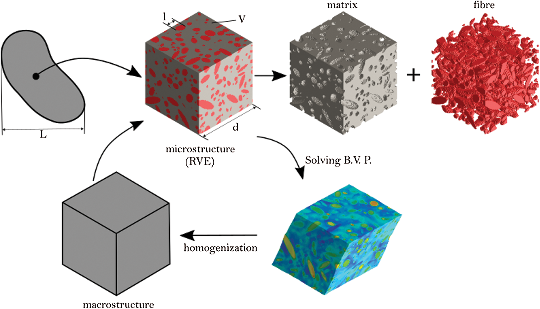
Figure 1: Principle of a homogenisation schema
This work aims at studying the mechanical properties of a WPC made from recycled PET and Chilean radiate pines’ flour, considering different weight fractions, sizes and aspect ratios of wood particles. The numerical prediction uses the DIGIMAT-FE software to generate the RVE and to solve the discretized finite element problem with periodic boundary conditions. WPC specimens are manufactured using a 16-mm twin-screw extruder and injection moulding, then characterised by static 3-point bending tests. The paper has the following outline: Section 2 summaries the numerical homogenisation methodology, while the experimental strategy is introduced in Section 3. The numerical and experimental comparison is addressed in Section 4. Finally, conclusions are drawn in Section 5.
This Section deals with the hypothesis and main features of the computational framework.
As previously described by the authors in [32], the simplest point of view for homogenisation is that a heterogeneous medium behaves macroscopically in the same way as its constituents. In micromechanical analysis, the stress and deformation fields of heterogeneous materials are divided into contributions from different scales. It is assumed that these scales are sufficiently different, i.e., with high and low wavelength effects such that: (i) fluctuations of fields in the microscale have influence at the macroscopic behavior only through its volumetric average; (ii) the gradients of the stress and deformation fields at the macroscale are not significant at the micro level, where these fields appear to be constant. These assumptions allow to define scale transitions through a BVP with prescribed displacements of some characteristic points at the boundary of the RVE, using a volume average of deformations or stresses and of the virtual work [29] (Hill–Mandel principle of macrohomogeneity [33,34]).
Before obtaining EEPs of a heterogeneous material, the size of the RVE should be studied in order to find the appropriate dimensions whose EEP is objective. This RVE must contain enough heterogeneity and its size d must be much larger than the characteristic length l of the microscale. Then, the RVE must be small enough to be assimilated to a point at the macroscopic level. A characteristic length L at this level can be determined according to the geometry, the spatial variation in loads or through the strain or stress fields. In fact, scale separation is verified when  , as schematized in Fig. 1.
The simplest mean-field homogenisation methods are the Voigt [35] and Reuss [36] models. Voigt assumes that the strain field is uniform in the RVE; consequently, the macro stiffness is found to be the volume average of the micro stiffness. In the Reuss model, the stress field is assumed to be uniform in the RVE; the macro compliance is then found to be the volume average of all micro compliance. The EEPs calculated are straightforwardly identified as the upper (Voigt) or the lower (Reuss) bound, respectively. These methods are easily implemented but they do not take into account the shape or the orientation of inclusions.
In this work, the efforts are on understanding the mechanisms that dominate the macroscopic properties of the material, but that really arise from its microscopic composition. We propose to generate RVEs as real as possible using the DIGIMAT-FE software. Then, the finite element model is solved by a finite element analysis in the same software. Periodic boundary conditions are imposed on all faces of the RVE through a large set of equations that relate the degrees of freedom of nodes on opposite sides. Fig. 2 shows the six macroscopic strains applied to an RVE. Periodic boundary conditions generally lead to the best predictions when compared to Dirichlet, Neumann or mixed edge conditions. It also shows a faster convergence speed as the size of the RVE increases, but at the expense of greater CPU time and memory requirements due to the large set of constraints that must be imposed [37].
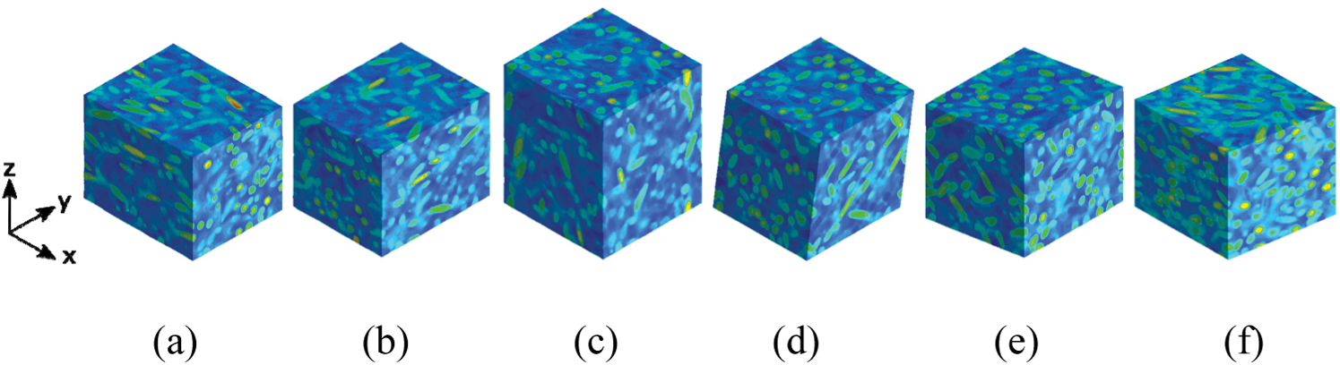
Figure 2: Deformed meshes of a RVE under periodic boundary conditions. Strains modes along planes: (a) x − x, (b) y − y, (c) z − z, (d) y − z, (e) x − z and (f) x − y
2.2 Particles’ Geometry and Size/FE-mesh of the RVE
In order to approach wood particles’ geometry, an ellipsoidal shape with transversely isotropic material properties is assumed—see Fig. 3a—where the longitudinal material direction coincides with the principal direction of the ellipsoid. From a geometric point of view, the parameters are shape (i.e., length and AR) and orientation of a particle. For the latter, two possibilities are studied: (i) 3D randomly distributed particles and (ii) particles slightly oriented to take into account flow effects due to the fabrication process (i.e., a degree of orientation non-null).
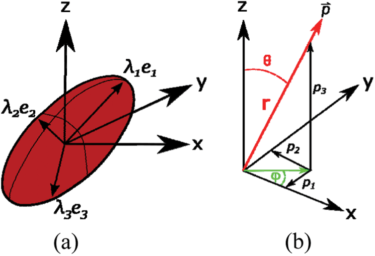
Figure 3: (a) Particle orientation. (b) Particle representation by a unit vector (p1, p2, p3) in an orthogonal coordinate system or (1,  ,
,  ) in a spherical coordinate system [38]
A 3D ellipsoid can be described by a second order tensor A—so-called orientation tensor—and its associated eigenvalue problem, as follows [38–40]:

where the eigenvectors ei indicate the principal directions of the particle’s alignment, while the eigenvalues  give the statistical proportions (0 to 1) of particles aligned with respect to those directions (a graphical representation is shown in Fig. 3a). A predominating orientation determines a respective eigenvalue close to 1, if the probability is weak it has a value close to 0. For a random distribution
 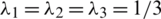 .
.
The nine components of the orientation tensor are reduced to five in dependent components due to symmetry (aij = aji) and the normalization condition (axx + ayy + azz = 1). A particle can be represented in space as schematised in Fig. 3b, where Cartesian coordinates can be retrieved from the spherical ones using  ,
,  and
and  . Finally, the orientation tensor can be defined as a dyadic product of the unit vectors as follows:

Note: the Cartesian coordinate system  is here chosen to be coincident with the injection’s flow of the specimens (see Section 3.3).
Another parameter is the degree of orientation OD which is a scalar value describing the strength of the main orientation of a tensor. It is calculated by the largest eigenvalue represented by  . Then, the degree of orientation can be obtained as follows:

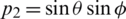
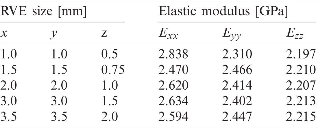
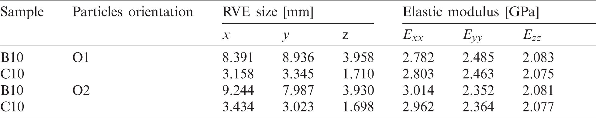
Before carrying out numerical homogenisation, the size of the RVE is firstly studied in order to find the minimal size for which EEPs converge, some examples are shown in Fig. 4. These RVEs are obtained using the automatic generation of periodic RVE from the commercial DIGIMAT-FE software. Tab. 1 surveys the chosen dimensions for each composite formulation defined in Section 3 (see Fig. 7a and Tab. 3), after studying different sizes which are summarised in Tabs. A.8–A.11. It is important to note that cubic RVEs are preferred for random particles, whereas rectangular ones are chosen for oriented distributions (see Tab. 7).
Figure 4: RVE with 10% of particles content (based on weight), but different side lengths: (a) 1.0 [mm]; (b) 1.5 [mm]; (c) 2.0 [mm]; (d) 2.5 [mm]; (e) 3.0 [mm]; (f) 3.5 [mm]; (g)  [mm]; (h)
  [mm]; (i)
  [mm]; (j)
  [mm]; (k)
  [mm]
[mm]
Table 1: Chosen dimensions for each RVEa

aA, B and C correspond to the complete line of sieves, particles retained from the 25 and 60 m, respectively (see Section 3.1). While O1, O2 and O3 correspond to the different orientation tensors used (see Tab. 7).
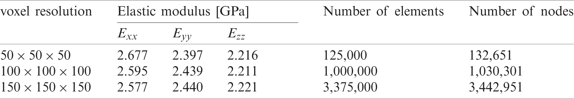
Voxelization modelling is advisable to support FE based simulations for complicated models. Taking into account the available computational resources and a previous convergence study of the homogenised elastic modulus (see Tab. A.12), the minimum RVE mesh resolution is selected to  voxels (for x, y and z directions) and it is used in all numerical homogenisation in this paper, as the one in Fig. 5.
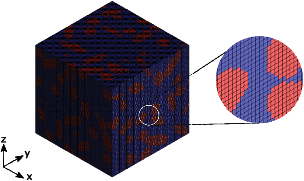
Figure 5: RVE’s voxelization modelling for C10 composite
Specimens are here detailed taking into account elastic properties, weight fractions, particles geometry, space distributions and the manufacturing processes as well.
Reinforce is wood flour which is a waste product of post-industrial operations such as sawing or milling. Wood flour here considered is made of Radiata pine, finely pulverized and with a 1% based on weight moisture content (after being dried in an oven at 100 [ C] for 24 h). Elastic properties taken into account are from the available literature [41], but simplifying wood as a transversely isotropic material because the ellipsoidal assumption made in Section 2.1, as follows: longitudinal and transverse Young’s modulus Exx = 11.059 [GPa], Eyy = 1.201 [GPa]; Poisson’s coefficients
  [ −],
[ −],  [ −]; transverse shear modulus Gxy = 1.339 [GPa]; and density 419.9 [kg/m3].
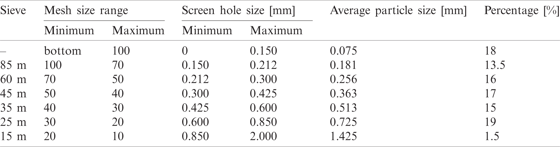
The size of the wood flour is first characterised through a sieving process, according to the ASTM E-11 specification [42], for which the mesh notations and corresponding screen sizes are shown in Tab. 2. More precisely, a 45 m sieve enables particles pass through a 40-mesh (0.425 [mm]), but not a 50-mesh (0.3 [mm]), then it holds particles with an average size of 0.363 [mm]. The resulting particle-size distribution after sieving the wood flour samples is in Tab. 2 (last column) and illustrated in Fig. 7b, where the mean size (i.e., width) of the probability distribution is 0.377 [mm].
Table 2: Mesh sizes used to sieve [42] and wood flour size distribution under study (last column)
WPC were produced using (i) the complete line of sieves (sample A), i.e., particles without sieving; and (ii) particles retained by the 25 and 60 m sieves, respectively. In order to better characterise the size and AR, wood flour from the 25 m (sample B) and 60 m (sample C) sieves were measured with an optical microscope Leica EZ4E (see Fig. 6). In the same way, an aleatory sample from the complete line of sieves was measured in order to estimate an average AR. Fig. 7a summarises these parameters for the three wood flour samples employed to manufacture composites. However, it is important to notice that the length and AR being prior to the compounding process, thus the particle geometry after processing could differ from the initial one due to the induced energy within the extrusion and injection process [43].

Figure 6: Optical measurement of particle’s geometry. (a) 25 m sieve (sample B) (b) 60 m sieve (sample C)
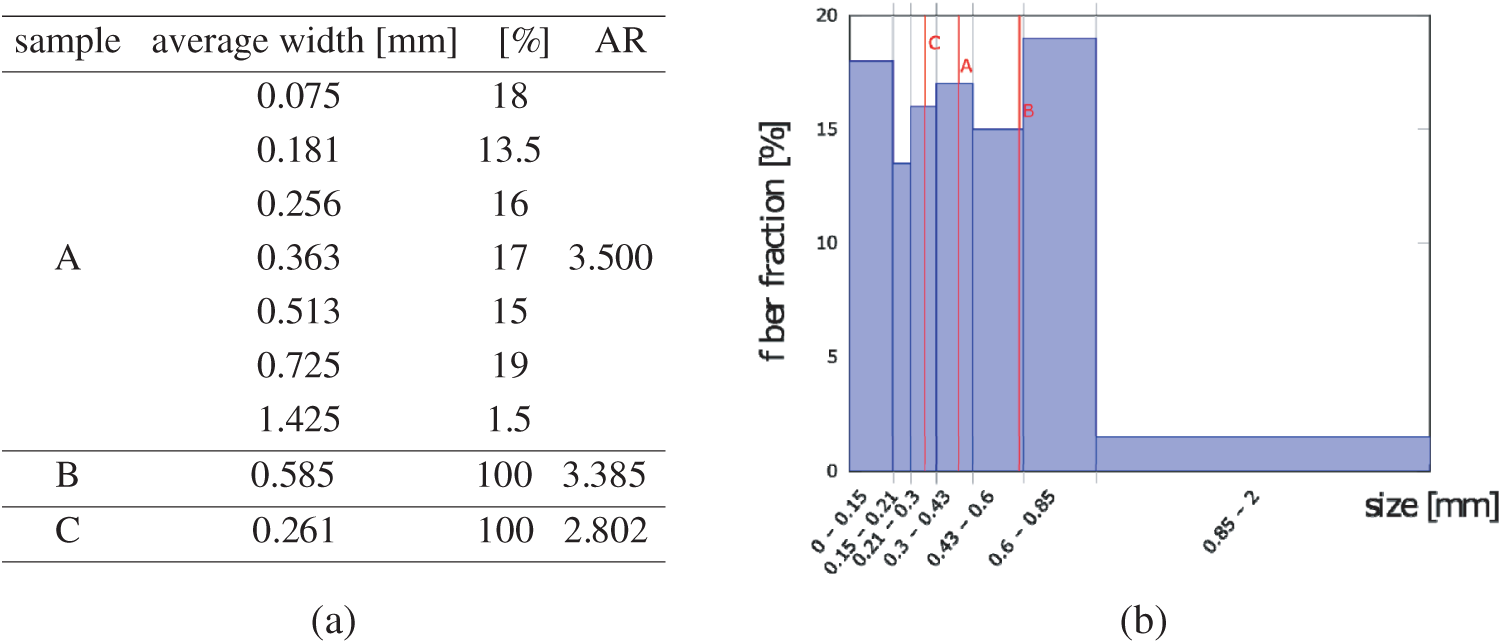
Figure 7: (a) Mean width and AR of three wood flour compositions. (b) Wood flour size (i.e., width) distribution according to Tab. 2. Red lines indicate the mean width of particles belonging to A, B and C compositions
The polymer matrix is a virgin polyethylene terephthalate (PET), with the following properties from literature [44]: viscosity 0.82 [dl/g], melting temperatures between 240–260 [ C], Young’s module
  [GPa] and Poisson’s coefficient
  [ −].
[ −].
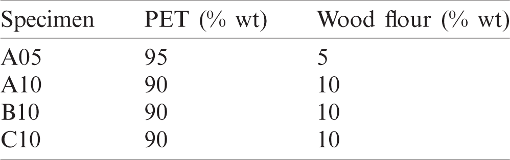
According to Tab. 3, two ratios of weights (5% and 10%) of wood flour and PET are studied for the size distribution A, although particles with a fixed size (B and C) are used to prepare composites with a wood content of 10% based on the total composite weight.
Table 3: Composition of WPC specimens
A laboratory extruder, TS 16–30 model (Gülnar Makina, Turkey), equipped with a twin-screw diameter of 16 [mm] and a single screw volumetric feeder was employed to manufacture the WPC. The extruder has three main zones, as schematised in Fig. 8: (i) Feeding, where material is preheated during transport; (ii) compressing, where material is compacted while decreases the screw depth; and (iii) dosing, where pressure is applied on materials shoving it towards the header. The volumetric feeder is used to nourish—as constant as possible—the mixture into the first zone. PET and wood were manually premixed prior to extrusions. Finally, the output is a continuous WPC filament with a diameter of 3.0 [mm]. The temperature profile is shown in Fig. 8, while the rotational speed was fixed to 20 [rpm].

Figure 8: Schematic diagram of the extruder machine
Specimens were moulded in a 490–170 Clarke 25 injection moulding machine at 237 [ C], according to Fig. 9 where the dotted arrows represent the injection flow. The geometry is in concordance with the 3 points bending tests defined in the ASTM D790 standard [45], with the following dimensions:
  [mm],
[mm],  [mm] and
  [mm] (see Fig. 9).
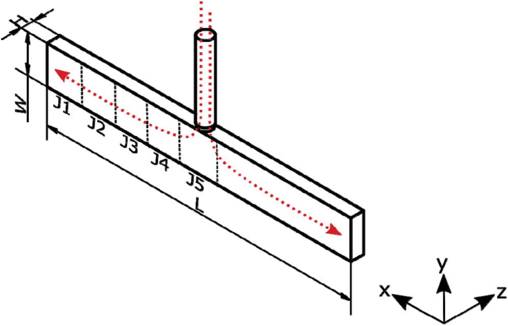
Figure 9: Specimens geometry, injection flow and zones for measuring the particle’s orientation
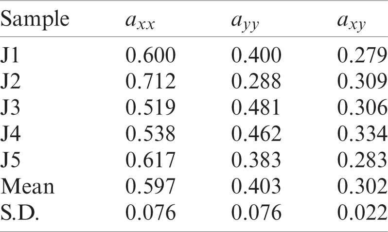
The distribution of the wood particles within the plastic matrix is here analysed. For the sake of simplicity, it is assumed that particles do not have an inclination in the z-direction, therefore only particles on the surface (x −y plane) are examined using an optical microscope Leica EZ4E. The surface is divided into five areas (see Fig. 9) for a better image resolution and software GeoGebra is employed for post-processing, as shown in Fig. 10. This procedure has been only achieved for specimens A05, because a low contrast on images was seen for samples with a wood content of 10%. Finally, components of the orientation tensor are calculated by means of Eq. (2), as detailed in Tab. 4. It is observed that particles are preferentially oriented with the x-direction, i.e., into the flow direction.
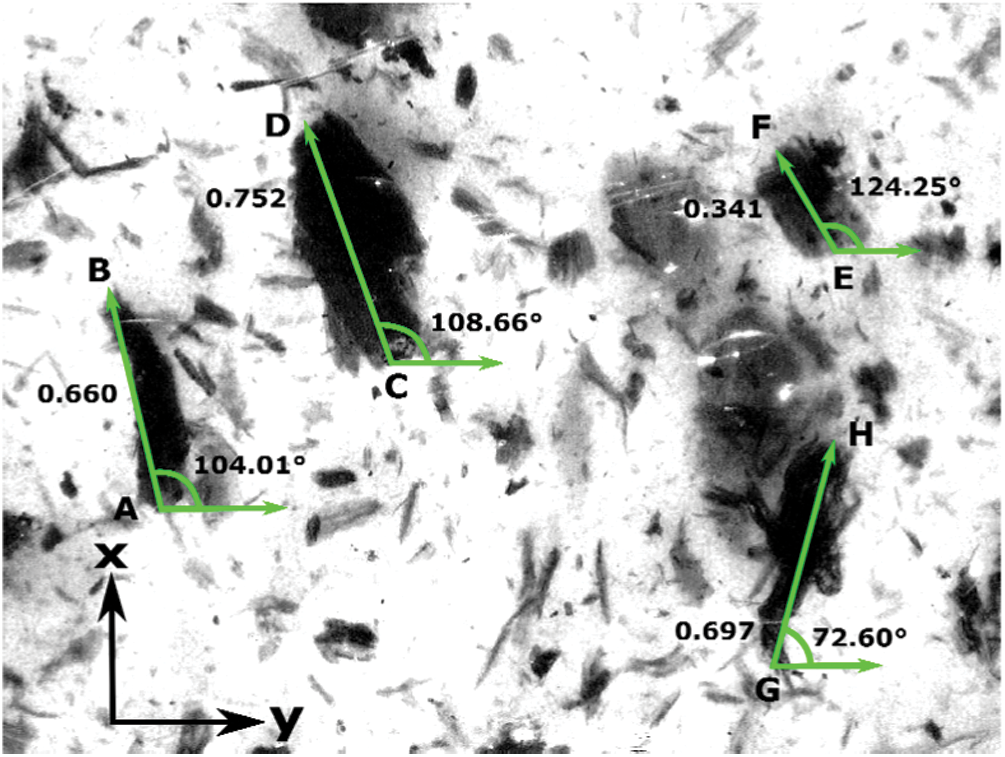
Figure 10: Image processing (plane x −y) in part of zone J5 for obtaining the fibre orientation tensor of an A05 specimen. (For interpretation of the color lines, the reader is referred to the web version of this article.)
Table 4: Fibre orientation tensor for different zones and its standard deviation (A05sample)
In this section an experimental and numerical comparison is addressed for the WPC manufactured in this work. Experiments are carried out according to the ASTM D790 standard [45], while simulations of elastic properties are performed in the DIGIMAT software.
Flexural strength measurements were obtained through 3-point bending tests in a testing machine—model Zwick Roell from Germany—provided with a 5 [kN] load cell and the testXpert software. The support span was 16 times (i.e., 56 [mm]) the specimen depth ( [mm], see Fig. 9) and the load speed was 1 [mm/min]. For each WPC in Tab. 3, five specimens were tested. Tab. 5 summarises the flexural modulus—i.e., the elastic module in x-direction −, the flexural strength and the elongation at the break foreach composite and for a specimen made of 100% PET as well.
Table 5: Mechanical properties and their standard deviations (3-point bending tests)
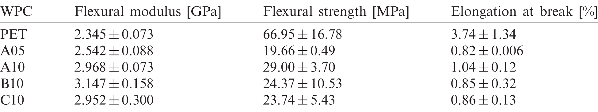
The Young’s modulus of PET is in concordance with available information [44]. When adding 5% wt. (10% wt., respectively) of wood particles to the PET matrix, the flexural modulus increases 8.0% (26.1% as average, respectively) respect to PET. It is then verified that the flexural modulus not only increases with the wood flour content, but also with the size of the wood particles. In fact, B10 samples have particles 124.14% bigger than those of C10, then its elastic module is 6.6% bigger than C10 specimens. If particles are not sieved (case A10), the elastic modulus is similar to the one of the C10 samples.
On the other hand, the addition of wood flour decreases the flexural strength and the ultimate tensile elongation respect to a 100% PET specimen, but these properties are improved as the quantity of reinforcement is increased. Actually, if 5% wt. (10% wt., respectively) of reinforcement is considered, the strength is reduced by 70.63% (56.68% as average, respectively) while the elongation at break is reduced by 76.34% (70.0% as average, respectively), respect to PET. However, if wood flour with a larger distribution of sizes (case A10, see Fig. 7b) is considered, the flexural strength (19.0% and 22.16% higher than B10 and C10, respectively) and the elongation at the break (22.35% and 20.93% higher than B10 and C10, respectively) are improved. It is important to note that the standard deviations of flexural strengths increase for the sieved sizes (B10 and C10).
4.2 Numerical-Experimental Comparison
The comparison here achieved is based on the elastic module in x-direction (see Fig. 9). Experimental values are from Tab. 5 and simulations are carried out using a periodic homogenisation method in the DIGIMAT software, where RVEs are been carefully calibrated according to Section 2.1. The size of particles and its orientations are varied in simulations. Finally, the theoretical values from the Voigt and Reuss assumptions are also given as reference.
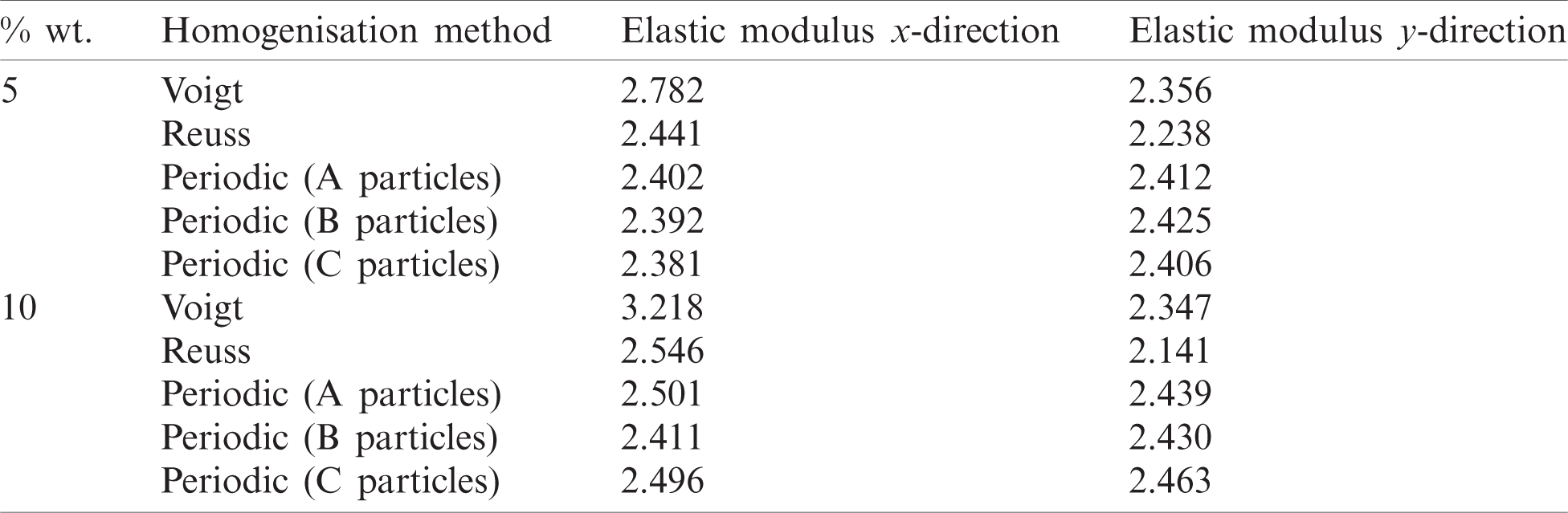
In order to study the influence of the particle sizes and their orientations, simulations taking into account a fully 3D random distribution of particles are first analysed. The modulus of elasticity in x and y directions are calculated for different particles sizes (see Fig. 7a), different wood content (5% and 10%) and using three homogenisation methods (Voigt, Reuss and periodic), as shown in Tab. 6. As previously found in [32], the periodic homogenised elastic moduli are almost the same in both directions—i.e., a quasi-isotropic composite material is obtained—and they are contained into the Voigt and Reuss bounds in the axial and transverse directions, respectively. For both wood content, the Young’s moduli obtained from periodic homogenisation are very close for the three-particle sizes (A, B and C). Finally, the elastic modulus increases as average a 2.08% (4.36%) if 5% wt. (10% wt., respectively) of wood is added to PET. Those results are significantly lower than the experimental ones, especially for the highest content of wood. In fact, the numerical elastic modulus is 5.31%, 16.78%, 23.09% and 16.01% lower than those measured experimentally for A05, A10, B10 and C10 compositions, respectively. This discrepancy can be explained because particles can choose a particular space orientation in agreement with the manufacturing process of specimens, as empirically verified in Section 3.4.
Table 6: Elastic modulus for different formulations with random particles’ orientation (periodic homogenisation is calculated with DIGIMAT software)
If a specific orientation is given to wood particles by indicating the orientation tensor into the periodic homogenisation routine in DIGIMAT software, the numerical elastic modulus is impacted. Indeed, Fig. 11 compares the elastic modulus in x-direction for the A05 and A10 composites, taking into account the experimental tests, the Voigt and Reuss bounds and numerical predictions with three orientations: fully random and the two configurations defined by the tensors detailed in Tab. 7, where it is important to note that the O1-orientation is according to the tensor found by image processing in Tab. 4 for a A05 specimen. Because particles are not spherical, it is observed that when more they are preferentially aligned into the injection flow direction, more the Young’s modulus increases. Actually, considering the orientation tensor O1 (O2), the numerical elastic modulus is 13.27% (20.39%, respectively) higher than the one with random arrangement. Finally, the prediction with O1-orientation (i.e., the one from image processing) is in agreement with the experimental Young’s modulus for the A05 composite. However, in the case of 10% of wood content, the O1-orientation does not match enough the empirical tests, but a simulation with a higher degree of particles’ alignment (i.e., the O2-orientation)is in conformity with the experimentation. This outcome could be explained under the hypothesis that the injection process induces particles to be oriented in the flow direction in a more severity way if wood content is added in a greater quantity.
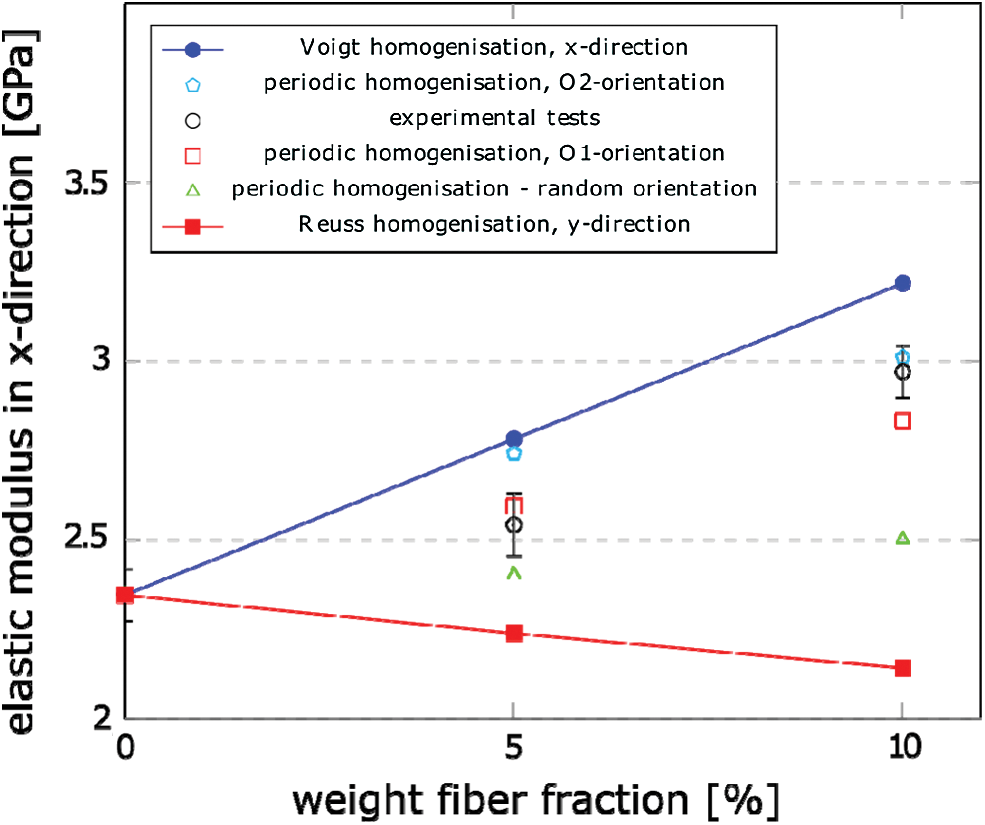
Figure 11: Numerical-experimental comparison of the Young’s modulus in x-direction for A05 and A10 composites. As in a random spatial distribution (O3), the results are considered contained between the Voigt and Reuss limits in the axial and transverse directions, respectively
Table 7: Orientation tensor used for periodic homogenisation in Fig. 11
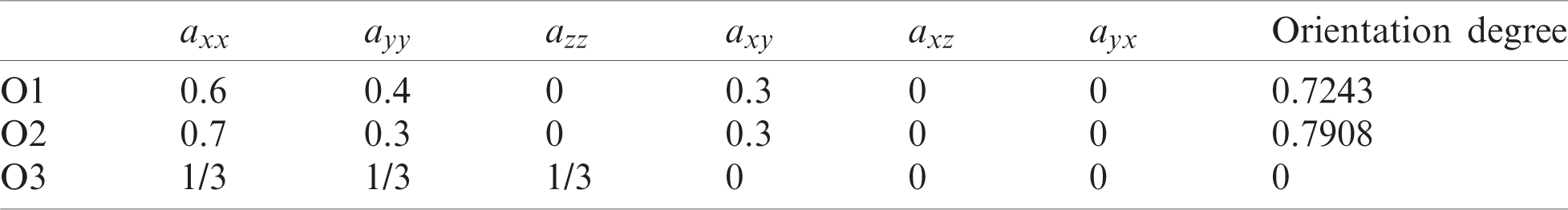
Fig. 12 shows the modulus of elasticity for WPCs with 10% wt. wood content and three different particle’s sizes—A, B and C (see Table in Fig. 7a)—where the periodic homogenisation method is checked against experimental results. Firstly, for each case (experimental, periodic homogenisation with O1-orientation or periodic homogenization with O2-orientation) it is verified that the Young’s modulus in x-direction for B10 is higher than for A10 composites, and the latter is higher than for C10 composites. Secondly, numerical predictions considering the O1-orientation underestimate the empirical values (except for C10), while O2-orientation matches the three experiments. However, B10 has the highest difference between the numerical and experimental mean values, then it can be assumed that C10 specimens have particles with a degree of orientation respect to the x-axis superior to 79% (see Tab. 7), according to Eq. (3). Furthermore, the simulation with random layout has the elastic modulus most weak. Finally, it can be concluded that for a fixed content of wood, the Young’s modulus in the flow direction increases when the average particle size increases.
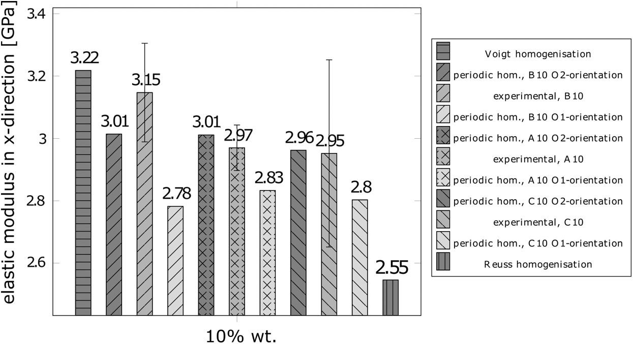
Figure 12: Influence of size and space orientation of particles on the Young’s modulus in x-direction for A10, B10 and C10 composites
This paper contrast numerical simulations and experimental testing for estimating the mechanical properties of a WPC manufactured with PET and Chilean Radiate pine’s wood flour. The influence of quantity, size and space orientation of particles on the elastic modulus was numerically predicted and then empirically validated. Simulations were carried out using a periodic homogenisation method combined with a finite element analysis, while 3 points bending tests were performed for obtaining elastic moduli, flexural strengths and the elongations at the break. Composites were manufactured with a laboratory extruder equipped with a twin-screw and specimens were then moulded by injection. The major outcomes of this work are:
—Experimentally, it has been verified that the elastic modulus not only increases with the wood flour content (8.0% and 26.1% for 5% wt. and 10% wt., respectively) of wood particles, but also with bigger particles.
—Experimentally, it is observed that the wood flour decreases the flexural strength hand the ultimate tensile elongation respect to 100% PET specimen, but these properties are improved as the quantity of reinforcement is increased. It is also verified that if particles are not sieved the elastic modulus is similar to other distributions, but the flexural strength and the ultimate tensile elongation are 20% improved (for composites with 10% wt. of wood).
—Numerically, considering random orientation, the elastic modulus increases as average a 10.24% and 19.20% if 5% wt. and 10% wt. of wood is added to PET respectively. However, those results are significantly lower than the experimental ones. This discrepancy is explained because the injection process induces particles to be oriented in the flow direction, especially if wood content is added in a greater quantity or using bigger particles.
—It is demonstrated that the homogenisation technique can predict the elastic moduli of wood PET composites. The experimental and numerical results are within the upper (Voigt) and lower (Reuss) limits. However, it can be very sensitive to the space orientation due to the manufacturing process of the samples, and it is necessary to carefully measure it as an input for simulations. Image processing using computed tomography could be a potential tool in order to have more accurate simulations [46–48].
Funding Statement: The authors wish to acknowledge the financial support from the Chilean Regional Government of Maule through the FIC-R project “Valorization of recycled waste through the creation of new materials for the manufacture of marketable products”, code BIP 30.481.945.
Conflicts of Interest: The authors declare that they have no conflicts of interest to report regarding the present study.
Contributions of Authors: P. P. carried out the experimental and numerical studies, contributed to the interpretation of the results, drafted the manuscript and designed the figures. K. S. designed the numerical tests and wrote the manuscript. G. P. conceived the experiments and helped to draft the manuscript. All the authors discussed the results.
1. S. Jarusombuti and N. Ayrilmis. (2011). “Surface characteristics and overlaying properties of flat-pressed wood plastic composites,” European Journal of Wood and Wood Products, vol. 69, no. 3, pp. 375–382. [Google Scholar]
2. K.-S. Rahman, M. Islam, M. Rahman, M. Hannan, R. Dungani et al. (2013). , “Flat-pressed wood plastic composites from sawdust and recycled polyethylene terephthalate (PETPhysical and mechanical properties,” SpringerPlus, vol. 2, no. 1, pp. 629. [Google Scholar]
3. M. Schwarzkopf and M. Burnard. (2016). “Wood-plastic composites: Performance and environmental impacts,” in A. Kutnar and S. S. Muthu, Environmental Impacts of Traditional and Innovative Forest-Based Bioproducts, Singapore: Springer, pp. 19–43. [Google Scholar]
4. A. A. Klyosov. (2007). Wood-Plastic Composites. Hoboken, New Jersey, United States: John Wiley & Sons, Ltd. [Google Scholar]
5. Y. Lei and Q. Wu. (2012). “High density polyethylene and poly(ethylene terephthalate) in situ sub-micro-fibril blends as a matrix for wood plastic composites,” Composites Part A: Applied Science and Manufacturing, vol. 43, no. 1, pp. 73–78. [Google Scholar]
6. I. Pogrebnyak, N. Sova, B. Savchenko, V. Pakharenko and V. Moisyuk. (2015). “A wood-filled composite based on recycled polyethylene terephthalate: Production and properties,” International Polymer Science and Technology, vol. 42, no. 1, pp. 41–43. [Google Scholar]
7. J. Cruz-Salgado, S. Alonso-Romero, R. Zitzumbo-Guzmán and J. Domínguez-Domínguez. (2015). “Optimization of the tensile and flexural strength of a wood-PET composite,” Ingeniería Investigación y Tecnología, vol. 16, no. 1, pp. 105–112. [Google Scholar]
8. F. L. Mantia and M. Morreale. (2011). “Green composites: A brief review,” Composites Part A: Applied Science and Manufacturing, vol. 42, no. 6, pp. 579–588. [Google Scholar]
9. S. K. Najafi. (2013). “Use of recycled plastics in wood plastic composites—A review,” Waste Management, vol. 33, no. 9, pp. 1898–1905. [Google Scholar]
10. W. Srubar and S. Billington. (2013). “A micromechanical model for moisture-induced deterioration in fully biorenewable wood-plastic composites,” Composites Part A: Applied Science and Manufacturing, vol. 50, no. 3, pp. 81–92. [Google Scholar]
11. OECD. (2016). Extended Producer Responsibility: Updated Guidance for Efficient Waste Management. Paris, France: OECD Publishing. [Google Scholar]
12. N. M. Stark and R. E. Rowlands. (2003). “Effects of wood fiber characteristics on mechanical properties of wood/polypropylene composites,” Wood and Fiber Science, vol. 35, no. 2, pp. 167–174. [Google Scholar]
13. H. Chen, T. Chen and C. Hsu. (2006). “Effects of wood particle size and mixing ratios of HDPE on the properties of the composites,” Holz als Roh-und Werkstoff, vol. 64, no. 3, pp. 172–177.
14. T. Mbarek, L. Robert, F. Hugot and J. J. Orteu. (2011). “Mechanical behavior of wood-plastic composites investigated by 3D digital image correlation,” Journal of Composite Materials, vol. 45, no. 26, pp. 2751–2764.
15. M. Schwarzkopf and L. Muszynski. (2015). “Strain distribution and load transfer in the polymer-wood particle bond in wood plastic composites,” Holzforschung, vol. 69, no. 1, pp. 53–60. [Google Scholar]
16. A. Schirp and J. Stender. (2010). “Properties of extruded wood-plastic composites based on refiner wood fibres (TMP fibres) and hemp fibres,” European Journal of Wood and Wood Products, vol. 68, no. 2, pp. 219–231.
17. J. Lisperguer, X. Bustos, Y. Saravia, C. Escobar and H. Venegas. (2013). “Efecto de las características de harina de madera en las propiedades físico-mecánicas y térmicas de polipropileno reciclado,” Maderas Ciencia y Tecnología, vol. 15, no. 3, pp. 321–336.
18. C. Pao and C. Yeng. (2018). “Properties and characterization of wood plastic composites made from agro-waste materials and post-used expanded polyester foam,” Journal of Thermoplastic Composite Materials, vol. 32, no. 7, pp. 951–966. [Google Scholar]
19. S. K. Yeh and R. Gupta. (2008). “Improved wood-plastic composites through better processing,” Composites Part A: Applied Science and Manufacturing, vol. 39, no. 11, pp. 1694–1699. [Google Scholar]
20. M. Hietala, J. Niinimaki and K. Oksman. (2011). “The use of twin-screw extrusion in processing of wood: The effect of processing parameters and pretreatment,” Bioresources, vol. 6, pp. 4615–4625. [Google Scholar]
21. M. Hietala, E. Samuelsson, J. Niinimaki and K. Oksman. (2011). “The effect of pre-softened wood chips on wood fibre aspect ratio and mechanical properties of wood-polymer composites,” Composites Part A: Applied Science and Manufacturing, vol. 42, no. 12, pp. 2110–2116. [Google Scholar]
22. S. Y. Leu, T. H. Yang, S. F. Lo and T. H. Yang. (2012). “Optimized material composition to improve the physical and mechanical properties of extruded Wood Plastic Composites (WPCs),” Construction and Building Materials, vol. 29, no. 6, pp. 120–127. [Google Scholar]
23. J. D. Eshelby. (1957). “The determination of the elastic field of an ellipsoidal inclusion, and related problems,” Proc. of the Royal Society of London A: Mathematical, Physical and Engineering Sciences, vol. 241, no. 1226, pp. 376–396. [Google Scholar]
24. T. Mori and K. Tanaka. (1973). “Average stress in matrix and average elastic energy of materials with misfitting inclusions,” Acta Metallurgica, vol. 21, no. 5, pp. 571–574. [Google Scholar]
25. R. Hill. (1965). “A self-consistent mechanics of composite materials,” Journal of the Mechanics and Physics of Solids, vol. 13, no. 4, pp. 213–222. [Google Scholar]
26. Z. Hashin and S. Shtrikman. (1963). “A variational approach to the theory of the elastic behaviour of multiphase materials,” Journal of the Mechanics and Physics of Solids, vol. 11, no. 2, pp. 127–140. [Google Scholar]
27. O. Pierard, C. Friebel and I. Doghri. (2004). “Mean-field homogenization of multi-phase thermoelastic composites: A general framework and its validation,” Composites Science and Technology, vol. 64, no. 10, pp. 1587–1603. [Google Scholar]
28. S. Kammoun, I. Doghri, L. Adam, G. Robert and L. Delannay. (2011). “First pseudo-grain failure model for inelastic composites with misaligned short fibers,” Composites Part A: Applied Science and Manufacturing, vol. 42, no. 12, pp. 1892–1902. [Google Scholar]
29. M. Geers, V. Kouznetsova and W. Brekelmans. (2010). “Multi-scale computational homogenization: Trends and challenges,” Journal of Computational and Applied Mathematics, vol. 234, no. 7, pp. 2175–2182. [Google Scholar]
30. R. Pucha and J. Worthy. (2014). “Representative volume element-based design and analysis tools for composite materials with nanofillers,” Journal of Composite Materials, vol. 48, no. 17, pp. 2117–2129. [Google Scholar]
31. C. Soyarslan, M. Pradas and S. Bargmann. (2019). “Effective elastic properties of 3D stochastic bicontinuous composites,” Mechanics of Materials, vol. 137, no. 2, pp. 103098. [Google Scholar]
32. P. Pesante, K. Saavedra, G. Pincheira, J. Hinojosa and C. Retamal. (2020). “Computational homogenisation of a recycled composite material based on PET and wood particles,” in Pro. of the 6th European Conf. on Computational Mechanics: Solids, Structures and Coupled Problems, 2018 and 7th European Conf. on Computational Fluid Dynamics, Glasgow, UK, pp. 2326–2336. [Google Scholar]
33. J. Mandel. (1972). “Plasticité classique et viscoplasticité,” in Course held at CISM. Udine: Springer-Verlag. [Google Scholar]
34. R. Hill. (1963). “Elastic properties of reinforced solids: Some theoretical principles,” Journal of the Mechanics and Physics of Solids, vol. 11, no. 5, pp. 357–372. [Google Scholar]
35. W. Voigt. (1889). “Ueber die beziehung zwischen den beiden elasticitätsconstanten isotroper körper,” Annalen der Physik, vol. 274, no. 12, pp. 573–587. [Google Scholar]
36. A. Reuss. (1929). “Berechnung der fließgrenze von mischkristallen auf grund der plastizitätsbedingung für einkristalle,” Zeitschrift für Angewandte Mathematik und Mechanik, vol. 9, no. 1, pp. 49–58. [Google Scholar]
37. MSC Software Company. (2018). “DIGIMAT User’s Manual,” . https://www.e-xstream.com. [Google Scholar]
38. W. Fracz and G. Janowski. (2017). “Analysis of fiber orientation in the wood-polymer composites (WPC) on selected examples,” Advances in Science and Technology Research Journal, vol. 11, no. 3, pp. 122–129. [Google Scholar]
39. S. G. Advani and C. L. Tucker. (1987). “The use of tensors to describe and predict fiber orientation in short fiber composites,” Journal of Rheology, vol. 31, no. 8, pp. 751–784.
40. J. Weissenböck, M. Arikan, D. Salaberger, J. Kastner, J. D. Beenhouwer et al. (2018). , “Comparative visualization of orientation tensors in fiber-reinforced polymers,” in Proc. of the 8th Conf. on Industrial Computed Tomography, Wels, Austria, pp. 1–9. [Google Scholar]
41. C. Fuentealba. (2001). “Determinación de las constantes elásticas en pinus Radiata D.Don por ultrasonido: módulos de elasticidad, módulos de rigidez y razón de poisson,” Maderas, Ciencia y Tecnología, vol. 3, pp. 1–2. [Google Scholar]
42. ASTM International. (2015). ASTM E11-15, Standard Specification for Woven Wire Test Sieve Cloth and Test Sieves. Conshohocken, PA West: ASTM International. [Google Scholar]
43. L. Teuber, H. Militz and A. Krause. (2013). “Characterisation of the wood component of WPC via dynamic image analysis,” in Proc. of the first Int. Conf. on Resource Efficiency in Interorganizational Networks, Göttingen, Germany, pp. 46–54. [Google Scholar]
44. Professional Plastics INC., “Mechanical properties of plastic materials,” [Online]. Available: https://www.professionalplastics.com/professionalplastics/MechanicalPropertiesofPlastics.pdf44. [Google Scholar]
45. ASTM International. (2017). “ASTM D790-17, Standard Test Methods for Flexural Properties of Unreinforced and Reinforced Plastics and Electrical Insulating Materials. Philadelphia, PA: ASTM International. [Google Scholar]
46. A. Alemdar, H. Zhang, M. Sain, G. Cescutti and J. Müssig. (2008). “Determination of fiber size distributions of injection moulded polypropylene/natural fibers using X-ray microtomography,” Advanced Engineering Materials, vol. 10, no. 1–2, pp. 126–130. [Google Scholar]
47. M. Krause, J. M. Hausherr, B. Burgeth, C. Herrmann and W. Krenkel. (2010). “Determination of the fibre orientation in composites using the structure tensor and local X-ray transform,” Journal of Materials Science, vol. 45, no. 4, pp. 888–896. [Google Scholar]
48. P. Evans, O. Morrison, T. Senden, S. Vollmer, R. Roberts et al. (2010). , “Visualization and numerical analysis of adhesive distribution in particleboard using X-ray micro-computed tomography,” International Journal of Adhesion and Adhesives, vol. 30, no. 8, pp. 754–762. [Google Scholar]
Appendix A. Detailed Numerical Results
Elastic moduli obtained by periodic homogenisation are here reviewed for the selection attempts related to the RVE size and RVE mesh. Compositions are referred to Fig. 7a and Tab. 3, while orientation is defined in Tab. 7.
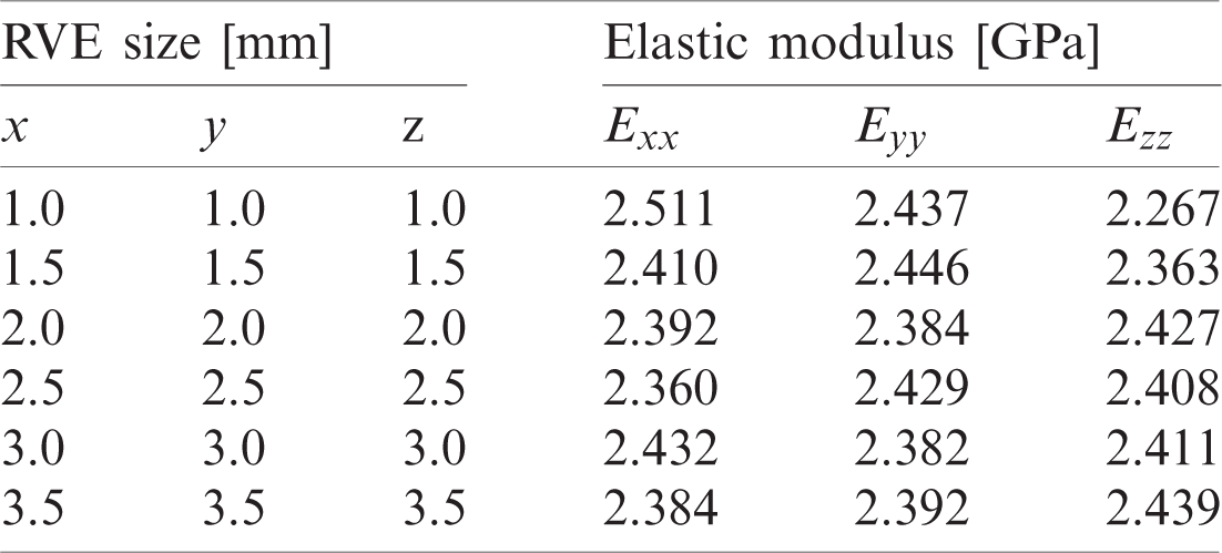
Homogenised elastic modulus for A05 composite and random distribution, different RVE dimensions
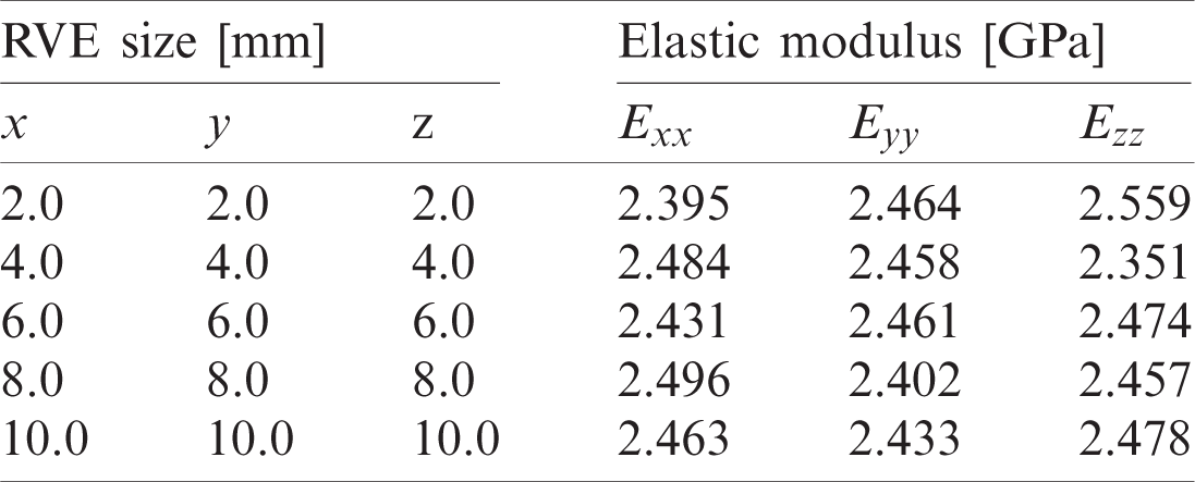
Homogenised elastic modulus for B10 composite and random distribution, different RVE dimensions
 | This work is licensed under a Creative Commons Attribution 4.0 International License, which permits unrestricted use, distribution, and reproduction in any medium, provided the original work is properly cited. |