Computers, Materials & Continua DOI:10.32604/cmc.2021.015174
Article

Time-Series Data and Analysis Software of Connected Vehicles

Jaekyu Lee1,2, Sangyub Lee1, Hyosub Choi1 and Hyeonjoong Cho2,*

1Korea Electronics Technology Institute, Seongnam-si, 13488, Korea
2Department of Computer Convergence Software, Korea University, Sejong-si, 30019, Korea
*Corresponding Author: Hyeonjoong Cho. Email: raycho@korea.ac.kr
Received: 09 November 2020; Accepted: 18 December 2020

Abstract: In this study, we developed software for vehicle big data analysis to analyze the time-series data of connected vehicles. We designed two software modules: The first to derive the Pearson correlation coefficients to analyze the collected data and the second to conduct exploratory data analysis of the collected vehicle data. In particular, we analyzed the dangerous driving patterns of motorists based on the safety standards of the Korea Transportation Safety Authority. We also analyzed seasonal fuel efficiency (four seasons) and mileage of vehicles, and identified rapid acceleration, rapid deceleration, sudden stopping (harsh braking), quick starting, sudden left turn, sudden right turn and sudden U-turn driving patterns of vehicles. We implemented the density-based spatial clustering of applications with a noise algorithm for trajectory analysis based on GPS (Global Positioning System) data and designed a long short-term memory algorithm and an auto-regressive integrated moving average model for time-series data analysis. In this paper, we mainly describe the development environment of the analysis software, the structure and data flow of the overall analysis platform, the configuration of the collected vehicle data, and the various algorithms used in the analysis. Finally, we present illustrative results of our analysis, such as dangerous driving patterns that were detected.

Keywords: Connected vehicle data; time series data; OBD data analysis; correlation coefficient

1  Introduction

Currently, massive amounts of data are collected and studied in various domains, including engineering, computer science, commerce, security, chemistry, and bio-molecular science. New datasets are constantly being generated and collected in various fields, and the amount of data is growing explosively. For example, global companies such as Google, Facebook, and Alibaba process tens of terabytes to hundreds of petabytes of data per day [1]. Big data is a term that describes massive amounts of data with large, varied, and complex structures that are difficult to collect, store, analyze, and visualize [2]. Big data was originally associated with three key concepts: volume, variety, and velocity of data, that is, the 3Vs model. Although big data is defined more comprehensively now, the “3Vs” model is still widely used by many enterprises, such as Gartner, IBM, and Microsoft [3]. In this study, we conducted time-series big data analysis using on-board diagnostic (OBD) data of connected vehicles. Based on the collected big data, we developed software and analyzed various parameters of connected vehicles. One of the main objectives of this study was to analyze data to derive valuable services related to automobiles. We have developed several applications, such as a Vehicle Arrival & Departure Service Platform/Real-Time Vehicle Monitoring System based on our software and the results of our analysis; we have recently expanded our work to related applications. The remainder of this paper is organized as follows. In Section 2, related work is described, and in Section 3, the structure of the big data analysis software, development environment, procedure for data processing (including preprocessing), and analysis software modules are described. In Section 4, the composition of the collected data is briefly described, and the results of various analyses are presented, including correlation coefficient analysis and dangerous driving pattern analysis. Finally, Section 5 presents the conclusions and discusses future research.

2  Related Work

In this section, we explore related research on vehicle big data analysis and the development of analysis software for vehicle big data. To date, little research has been reported on the analysis of OBD and GPS data of vehicles. Reference [4] presents an analysis of the driving behavior using the OBD data of vehicles and the AdaBoost (adaptive boosting) algorithm, which is a machine-learning meta-algorithm. The proposed method collects information about vehicle operation, including vehicle speed, engine RPM (Revolutions Per Minute), throttle position, and calculated engine load, via the OBD interface. They used data that were simulated using the OBD-II simulator rather than actual data; therefore, their method is somewhat limited. Another [5] presented a personalized driving behavior monitoring and analysis system for hybrid electric vehicles (HEVs). They proposed a method for capturing precise driver–vehicle information based on smartphone sensors; the system also provided quantitative driver-specific HEV analysis through operation mode classification, energy use, and fuel use modeling. Moreover, in a previous study, driver behavior was analyzed to improve vehicle safety [6]. The analysis was performed based on the collected data using a CAN (Controller Area Network) data recorder, and a system was developed for classifying drivers based on their behavior. However, although a CAN data recorder was used for the initial data acquisition, it was not implemented in the actual vehicle. Representative papers related to vehicle big data analysis are as follows. A big data framework for electric vehicle range estimation that can collect different data with various structures from numerous resources was proposed [7]. Another [8] reviewed state-of-the-art techniques used for handling big data of smart grids and electric vehicles. A big data approach for road accident hotspot identification using Apache Spark was reported [9]. However, it does not cover the development of vehicle big data analysis software, and most of the data used in these studies were simulated rather than being actual data.

We implemented the DBSCAN (Density-based Spatial Clustering of Applications with Noise), ARIMA (Auto-regressive Integrated Moving Average) model, and an LSTM (Long Short-Term Memory) algorithm to analyze time-series data. DBSCAN is a density-based data clustering algorithm. It is easy to find clusters with geometric shapes because this algorithm is clustered based on density [10]. Therefore, it is used in various fields; in this study, it was used to analyze the trajectory of the vehicle. LSTM is a recurrent neural network mainly used to analyze time-series data [11]. ARIMA, which is mainly used to predict time-series data, consists of autoregressive and moving average model [12]. The LSTM and ARIMA models are widely used to analyze and predict time-series data. A module was designed to self-diagnose parts of autonomous vehicles based on the LSTM algorithm [13]. The module diagnoses vehicle defects using time-series data, which is a correlation between previous diagnostic results of autonomous vehicle parts and currently measured data. A new ensemble three-phase model based on LSTM was proposed to improve the multivariate time-series prediction performance [14]. The proposed algorithm removes time-series noise using a new adaptive noise reducer (ANR), extracts features from time-series data using a stacked auto encoder (SAE), and proposes an ensemble model based on over-fitting prevention of LSTM. Vehicle interaction was modeled using a modified LSTM model for trajectory prediction [15]. The proposed spatiotemporal LSTM-based trajectory prediction model compensates for existing problems such as vanishing gradient problems and model inaccuracies in dense traffic. A method for analyzing and predicting traffic patterns in Los Angeles using machine learning and big data was proposed [16]. Here, Microsoft Azure ML was used to predict and classify traffic data patterns in Los Angeles. Azure ML provides users with a variety of algorithms (including the ARIMA model) for machine learning based on a GUI (Graphical User Interface). Novel denial-of-service (DoS) attack and distributed DoS (DDoS) attack detection algorithms using ARIMA time-series models and chaotic systems in computer networks were developed [17]. In the proposed algorithm, the ARIMA model is used to predict the number of packets every following minute. A time-series analysis method based on the ARIMA model was proposed [18], and the ARIMA model was applied to financial fields such as stock price prediction as a case study. These papers described the analysis of time-series data, even if they are not vehicle data. At this point, various discussions on time-series big data analysis of connected vehicles, efficient analysis methods, and analysis software development are needed. The data used in this study are reliable as they were collected from real vehicles driving on real roads. One of the main purposes of data analysis is to create new services through the analysis of collected data and to develop fully automated big data analysis software for connected vehicles. Currently, our big data acquisition platform is collecting and accumulating data from three different companies that operate different types of vehicles. However, we mainly analyzed the vehicle data from one company in this study. The results are described in this paper.

3  Development of the Analysis Software

In this section, we describe the overall development of the data analysis software. The structure of the entire system is illustrated in Fig. 1.

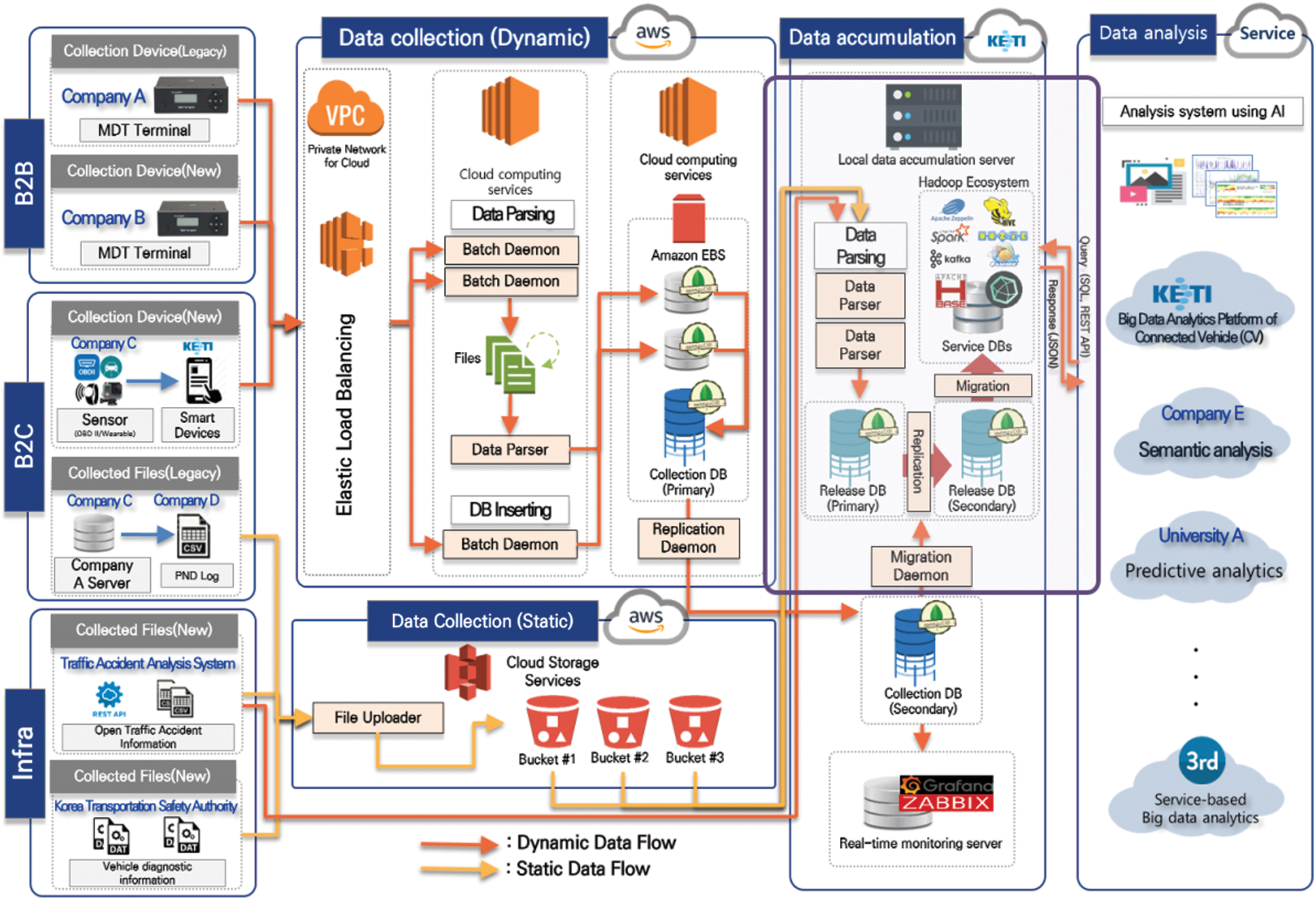
Figure 1: Configuration of the overall system

The system consists of data collection, analysis, and visualization software blocks. The data flow from data collection to analysis software as shown in Fig. 1. A brief summary of the process is explained in this section. To collect big data from connected vehicles, we classified data sources into business-to-business (B2B), business-to-customer (B2C), and infra data according to the business models. We developed an interface module for collecting data from connected vehicles. Here, the B2B data includes data from OBD dashboard (OBD-II), mobile digital terminal (MDT), digital tacho graph (DTG), and personal navigation device (PND) depending on the type of IoT sensor terminal of the vehicle. B2C data can be collected from the driver’s wearable device and smartphone application. Infra data are collected from the Korea Transportation Safety Authority; this data consist of static files, such as .csv, .xlsx Excel, .json, and .txt. Next, we collected data by separating dynamic data and static data. The flow of dynamic data is as follows. The dynamic data are updated on a cloud server (Amazon EC2) every predetermined period (10 min) by the company collecting the vehicle data. They are uploaded to the server in the form of a .txt file rather than a database file. In general, the uploaded files are periodically parsed by the parsing module in the cloud server and accumulate in the database server. However, the data received from some vendors are not in the form of a file. Therefore, certain S/W modules have been developed that directly input data into the database. Thus, parsed files and data that are directly input to the database constitute a database of dynamic data. In addition, static data are uploaded to the cloud storage server (Amazon S3). The transferred data are also parsed by the parsing module and stored in the database. The reason for dividing and processing data statically and dynamically is to process data more efficiently because the data collection cycles for each type of data are different. The static and dynamic data are combined to form an integrated database, which is migrated to the local database server. Finally, the analysis software that we developed takes data from this local server, called the analysis server, and performs data analysis. The analysis results are stored in multiple distributed database servers.

3.1 Environment for Development and Analysis

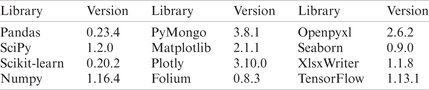
The analysis software was developed using Python 3.5; it is designed to be compatible with Python 2.7. Next, we used various libraries to develop our analysis software. The Pandas library was used to analyze large amounts of data efficiently; the Matplotlib and Plotly libraries were used to create graphs of the analysis results. In addition, we applied artificial intelligence techniques to our analysis software based on the SciPy, TensorFlow, Numpy, and Scikit-learn libraries as shown in Tab. 1. The results of the trajectory analysis using the DBSCAN algorithm (GPS-based) were visualized based on the Folium library, which makes data that has been manipulated in Python easy to visualize.

Table 1: Major libraries and versions used on our platform

3.2 Structure of Data Processing

In this study, three database platforms, MongoDB, InfluxDB, and Open TSDB, were used for data collection and storage of processed data. The raw data are collected and accumulated in each database, and the data processed by the analysis software are stored in a new table or metric (or measurement). InfluxDB is an in-memory database that enables very fast data processing, whereas OpenTSDB can efficiently store and process time-series data [19]. In addition, we used MongoDB, the performance of which is superior to that of a relational database and does not require schema management. In addition, the sharding technology, known as horizontal partitioning technology, was applied to the database to increase the scalability and availability of the database. We need to consider the availability and efficiency of the database because the collected vehicle data are intended for release through the Open API (Application Programming Interface) and RESTful (Representational State Transfer) API. Currently, this is expanding the big data collection and analysis system based on the Hadoop ecosystem. In particular, we applied Hbase, HIVE, and Apache ZooKeeper, which are known as subprojects of the Hadoop ecosystem, to our analysis platform (database and server).

3.3 Exploratory Data Analysis and Data Preprocessing

In this study, we performed exploratory data analysis (EDA) and data preprocessing before analyzing the data. The EDA and preprocessing tasks included removing not a number (NaN) and outlier data and creating new tags. In addition, we calculated the azimuth based on the GPS values because the current data only comprised GPS values without azimuth data. We calculated the azimuth using the GPS between two points [20,21]. The azimuth data were used to analyze the rotation of a car, such as a sharp left turn or a quick U-turn. The eight azimuth angles consist of north, northeast, east, southeast, south, southwest, west, and northwest.

3.4 Correlation Coefficient Analysis

We derived Pearson’s correlation coefficient before analyzing the data. The software module for obtaining the correlation coefficient was developed based on the following formula [22]:

where is Pearson’s correlation coefficient. E is defined as in Eq. (2).

Cov(X, Y) is the covariance of X and Y, is mean population x, is mean population y, is the standard deviation of population X, is the standard deviation of population Y, Z is the population, and the correlation coefficient has a value between −1 and 1 as follows:

The procedure for analyzing the correlation coefficient with other parameters based on the driving speed is shown in Fig. 2. The reason for analyzing Person’s correlation coefficient is to derive the correlation coefficient between each parameter and perform a more detailed analysis.

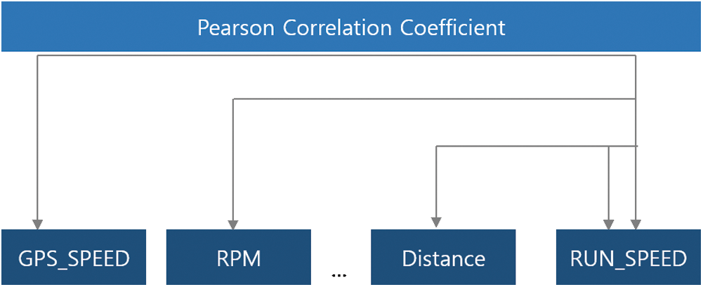
Figure 2: Correlation coefficient derivation

3.5 Development of Analysis Software Based on Time-Series Data

The structure and procedure of our analysis software are illustrated in Fig. 3. The procedure is briefly described as follows. First, the outliers (which are outside the data range of each parameter) are removed from the collected data. Then, a preprocessing operation is performed in which new tags are attached to the processed data. Each step of data preprocessing is carried out in parallel, and the newly tagged data are stored in a new table (or metric). Next, the data are analyzed on an analysis engine, which is a collection of various analysis methods and algorithms. The analysis engine includes algorithms to detect dangerous driving patterns, such as rapid acceleration, rapid deceleration, sudden starting, and sudden stopping. It also includes various machine-learning algorithms we have implemented, such as k-nearest neighbor, multilayer perceptron (MLP), support vector machine (SVM), decision tree, and trajectory analysis modules.

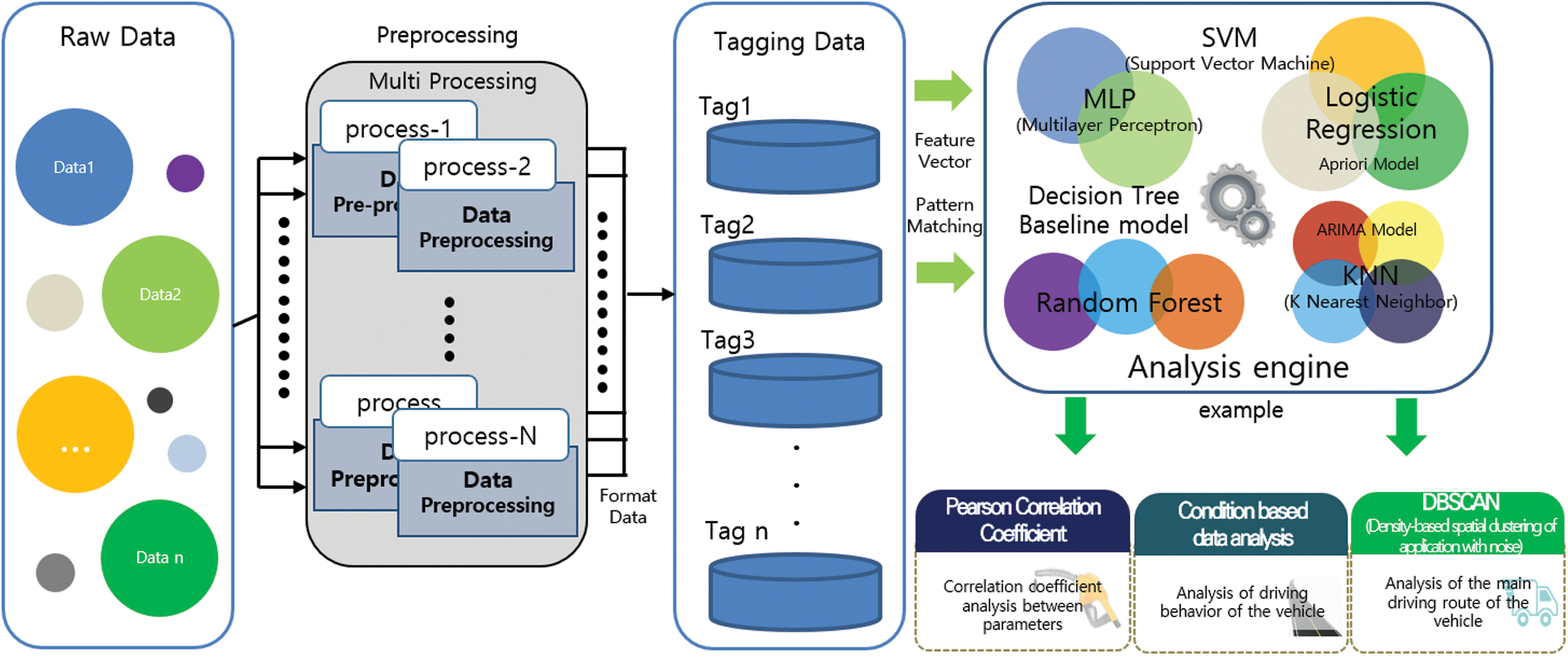
Figure 3: Structure of the analysis software

In particular, we implemented the DBSCAN algorithm, ARIMA model, and LSTM algorithm for time-series data analysis. As mentioned earlier, DBSCAN was used to analyze the trajectory of the vehicle in this study. We used the ARIMA model and LSTM to predict the battery voltage, coolant temperature, and engine oil temperature of the vehicle. Nevertheless, not all the algorithms we have implemented are used in the analysis engine and research on how to apply the most suitable algorithm to analyze the data we have collected is currently in progress.

4  Analysis Results

In this section, we describe representative results of our analysis, including the results of dangerous driving patterns.

4.1 Data Configuration

The main distribution of the collected data was as follows: The data collection period was from January 2017 to February 2020; the data were collected from three companies. Currently, the size of the dataset is approximately 73.1 GB with 793,138,471 rows (as of February 2020). The types and amounts of data parameters collected by each company are different. The monthly data distribution is shown in Fig. 4. The x- and y-axes represent time and the number of rows of data, respectively.

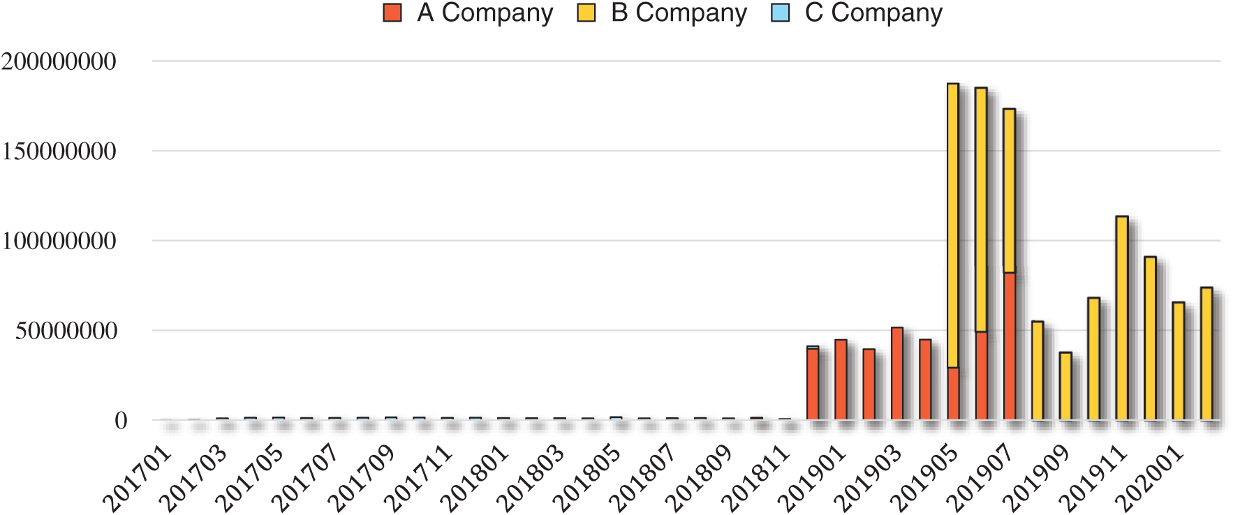
Figure 4: Distribution of the collected data

Tab. 2 lists the columns (field names) of automobile data we collected from Company C. Currently, the data field names and quantities for each company are slightly different. We are trying to standardize the data format. In addition, various preprocessing and post processing operations are necessary because not all data are completely input into the database. Tab. 2 presents all the data fields that can be collected when the data are in the ideal form. The data column is composed of up to 48 columns. The description of the field name is as follows. First, the collected vehicle data includes a car code (CAR_CD) for an automatic number, “CREATE_TIME” for the date and time when the data are created, and GPS-related information. The GPS information includes the latitude and longitude, GPS time, and GPS speed. The driving speed (RUN_SPEED), maximum speed (MAX_SPEED), and average speed (AVG_SPEED) of the vehicle are collected alongside data related to the driving distance (DRV_DISTANCE/DRV_DISTANCE_DAY/etc.). In addition, various data were collected, including the odometer (ODO) and cylinder load value (CLV), intake air temperature (IAT), and outside air temperature (OAT). Finally, data such as DTG SIGNAL and DTG_STATE columns and DEVICE_STATE, indicating terminal status, are accumulated.

Table 2: Field names of collected data

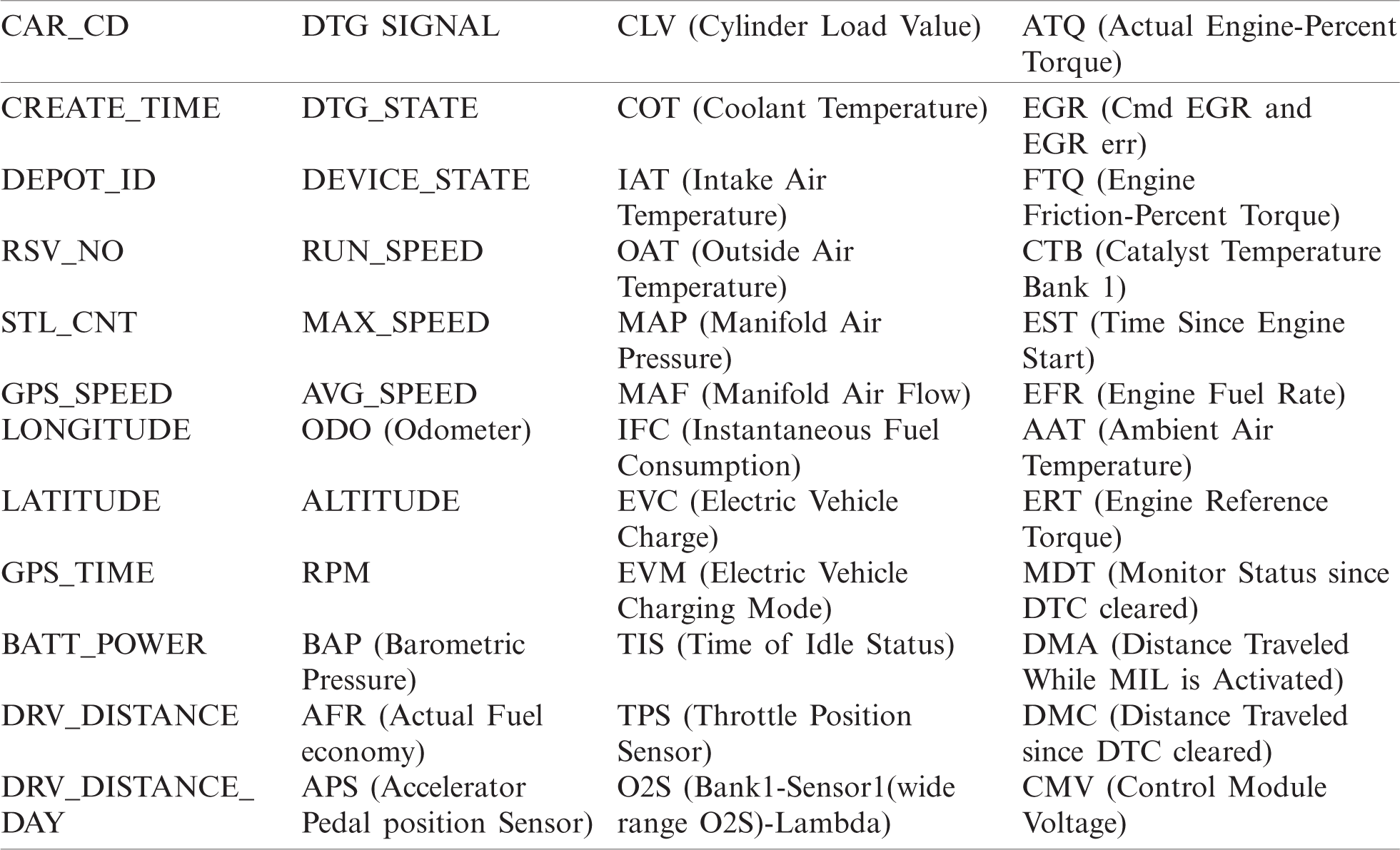
Although data columns related to electric vehicles exist, the data were not collected. Similarly, data were not collected for certain other data fields. In this study, the valid data among the collected data were analyzed. Among the collected data, preprocessing tasks, such as removing outliers and calculating GPS-based azimuth, were performed before analysis.

We plotted a histogram of the collected data to determine the distribution of the collected data and the composition of the field values as shown in Fig. 5. In the red graph, the overall data of each field are shown, and in the green graph, data excluding the zero value in the red graph are shown. The reason for removing the zero value is to enable the data to be inspected in detail. The data fields with a default value of zero have the highest proportion of zero values. Therefore, the distribution of all the data can be checked in detail by excluding the zero value. In Fig. 5, the field name is shown above each chart, and the x- and y-axes represent the data value of each field and the number of data in a given range, respectively. As shown in the charts relating to the driving speed, such as GPS_SPEED Histogram or RUN_SPEED Histogram, all vehicles traveled at a speed less than 175 km/h. This means that most of the collected speed data consist of values that do not exceed a maximum of 180 km/h. In addition, the histogram graph of the battery voltage or cylinder load value (CLV) field that can be seen in the red graph (including the 0 value) and green graph are almost the same. This is because the battery voltage is 27.7 V, not the default value of “0” as in the case of vehicle speed data (when the vehicle is stationary).

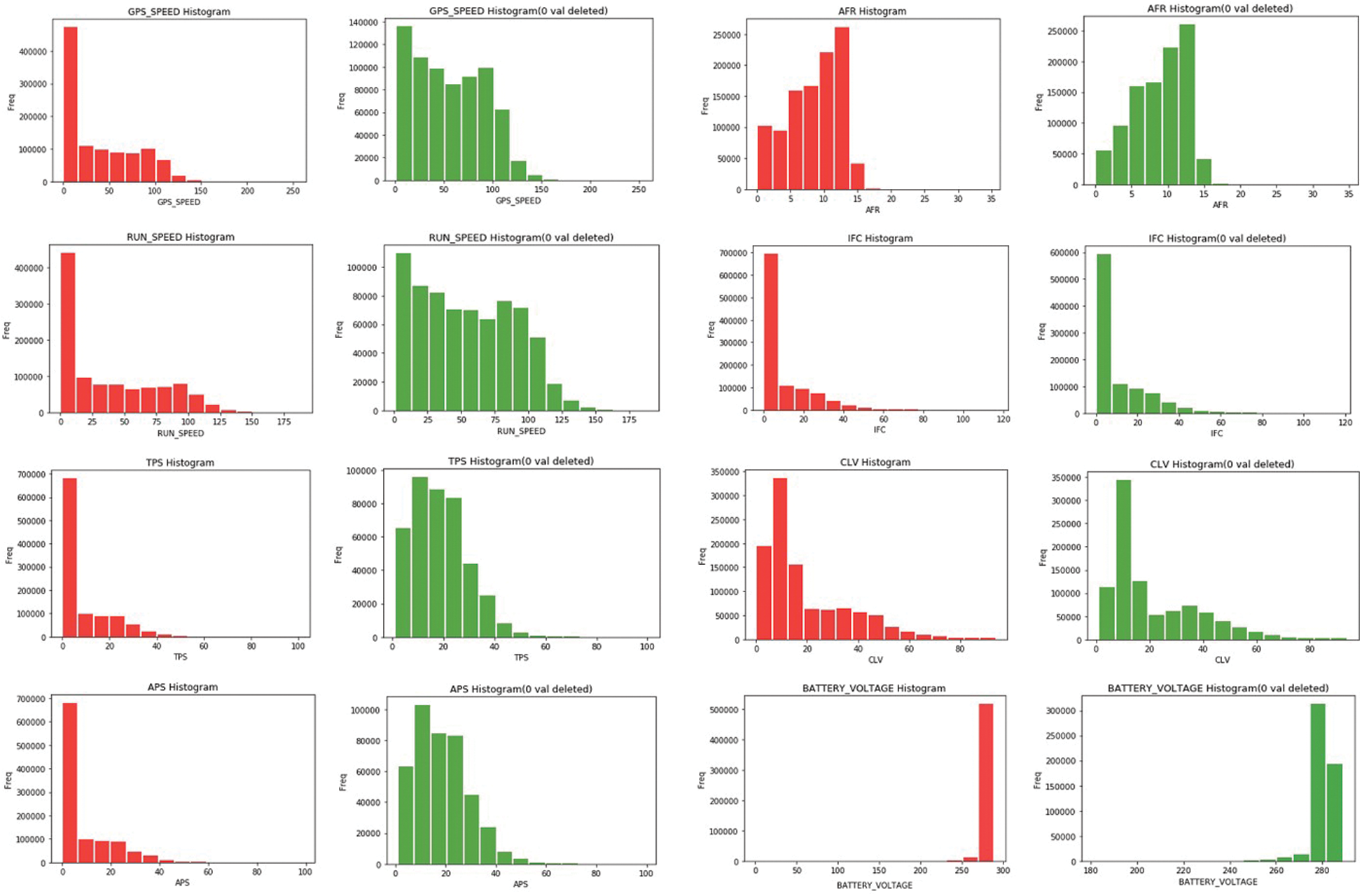
Figure 5: Data histograms (selected fields)

4.2 Correlation Coefficient

We analyzed the correlations using our S/W module based on Pearson’s correlation coefficient formula.

Fig. 6 (Graph A) shows the results of the correlation analysis based on the driving speed of a specific vehicle. The x- and y-axes represent the value of the correlation coefficient and the name of the data field used to measure the correlation coefficient, respectively. The results of the analyzed correlation coefficient can be summarized as follows: The parameter with the highest correlation with the running speed (RUN_SPEED) is RPM (0.731), and the positive correlation coefficient was highest in the order of instantaneous fuel consumption (IFC/0.714), accelerator pedal position sensor (APS/0.707), throttle position sensor (TPS/0.693), and cylinder load value (CLV/0.657). In addition, the outside air temperature sensor (OAT/ −0.525) has the highest negative correlation coefficient. This is because the faster the driving speed of the car, the lower the outside temperature generally becomes. This is interpreted as the decrease in outside temperature when the car is running at high speed. We have been expanding the analysis engine by clustering each parameter based on a correlation analysis module. A graph analyzing the correlation coefficient between the columns of the entire dataset is shown in Fig. 6 on the right (Graph B).

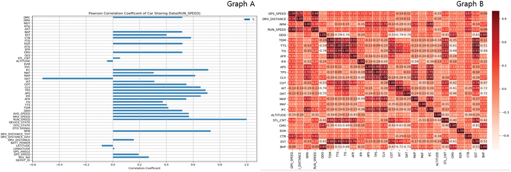
Figure 6: Pearson’s correlation coefficient

4.3 Analyzed Data

In this section, we present representative results of the various dangerous driving patterns we analyzed.

The dangerous driving behavior standard is that of the Korea Transportation Safety Authority [23]. Fig. 7 (graph1) shows the results of rapid vehicle acceleration. Vehicle 1384 had the highest number of rapid accelerations, followed by vehicles 11359, 11325, 11296, and 21356. In this graph, the x- and y-axes represent the vehicle number and the number of rapid accelerations, respectively. The results of the rapid deceleration analysis are shown in graph2 in Fig. 7, where the x- and y-axes represent the vehicle number and the number of rapid decelerations, respectively. The number of rapid decelerations was the highest for vehicle 11325; the number of rapid decelerations was relatively high for vehicles 1384 and 21356. Additionally, our analysis showed that a vehicle with a large number of rapid accelerations has a high number of rapid decelerations. Apart from this, analyzing the sudden starting and stopping (harsh braking) pattern of vehicles, we identified vehicle 11325 as having performed many sudden starts and stops. This finding enabled us to analyze the driver’s unique driving patterns. The results of analyzing the quick start pattern are shown in graph3 in Fig. 7, with the x- and y-axes representing the vehicle number and the number of quick starts, respectively. The largest number of quick starts was detected for vehicles 11325 and 1384, which, coincidentally, also had large numbers of rapid accelerations and rapid decelerations. This reflects the fact that vehicle drivers are known to have their own patterns. The results for the sudden stop pattern of the vehicles are shown in graph4 in Fig. 7. Vehicle 1367 had the highest number of sudden stops. In addition, the number of sudden stops was generally higher than the number of quick starts. In addition, the proportion of rapid decelerations among the number of quick starts, sudden stops, rapid accelerations, and rapid decelerations was the largest. Graph 4 in Fig. 7 presents the vehicle number and the number of sudden stops on the x- and y-axes, respectively.

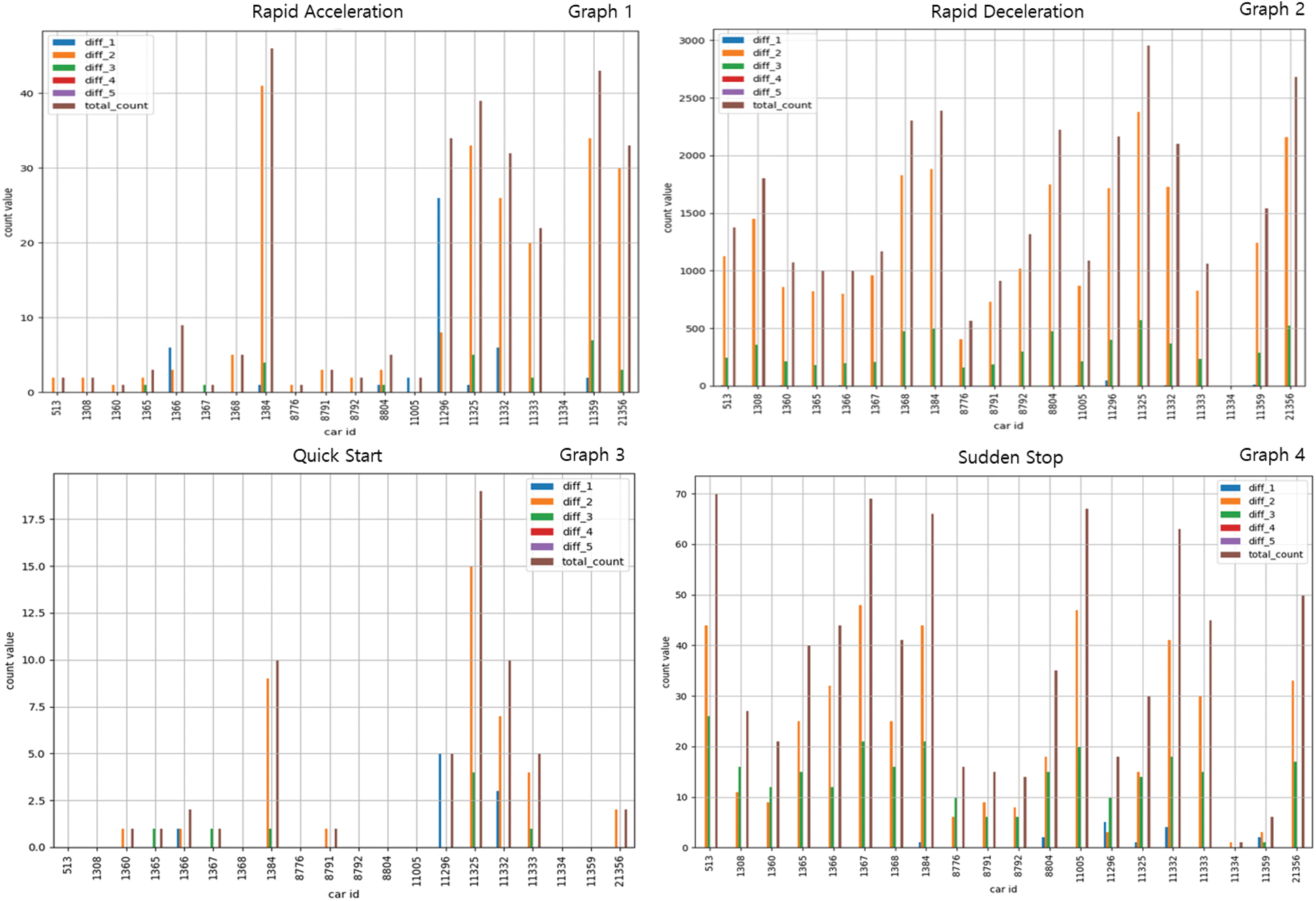
Figure 7: Driving behavior patterns

Fig. 8 (graph5) shows the results of our analysis of the sudden left or right turn patterns for each vehicle, with the x- and y-axes representing the vehicle number and the number of sudden left or right turns, respectively. This result was obtained by analyzing the data for 2017 and 2018. The blue and orange bars on this chart represent the number of sudden (sharp) left or right turns in 2017 and 2018, respectively. As shown in the graph, vehicle 11296 had the highest number of sharp left or right turns during these two years. Vehicle 8804 had the highest number of sharp left or right turns in 2017. Fig. 8 (graph6) shows the results for the sudden U-turn pattern and shows that, for these two years only vehicle 11332 showed a pattern of making sudden U-turns. In general, vehicle 11332 had a large number of rapid accelerations (within the top 32%), rapid decelerations (within the top 35%), quick starts (within the top 20%), and sudden stops (within the top 25%). Nevertheless, the sudden U-turn pattern had the lowest occurrence among the analyzed data. In graph, the x-axis represents the vehicle number, and the y-axis represents the number of sudden U-turns per year. Fig. 8 (graph7) shows the results of the seasonal analysis of the fuel economy of the vehicle, with the x-axis showing the vehicle number, and the y-axis the average fuel economy (km/l). These results are summarized as follows: vehicle 11332 had the highest fuel efficiency (approximately 22 km/l); the fuel efficiency of the vehicle was higher in summer (green) than in winter (red). The main reason for this is that the viscosity of the oils is higher at low temperatures. In addition, in winter, vehicles consume more fuel to preheat the engine than in summer, and the tire pressure is lowered, which translates into poor fuel economy. The developed software was designed to analyze the mileage of the vehicle as well as the mileage by period (yearly, monthly, daily). Fig. 8 (graph8) shows the annual mileage (km) of each vehicle (blue-green) and the monthly mileage of vehicle 1367 (pink). The most operated vehicle at 35,284 km per year was 11296.

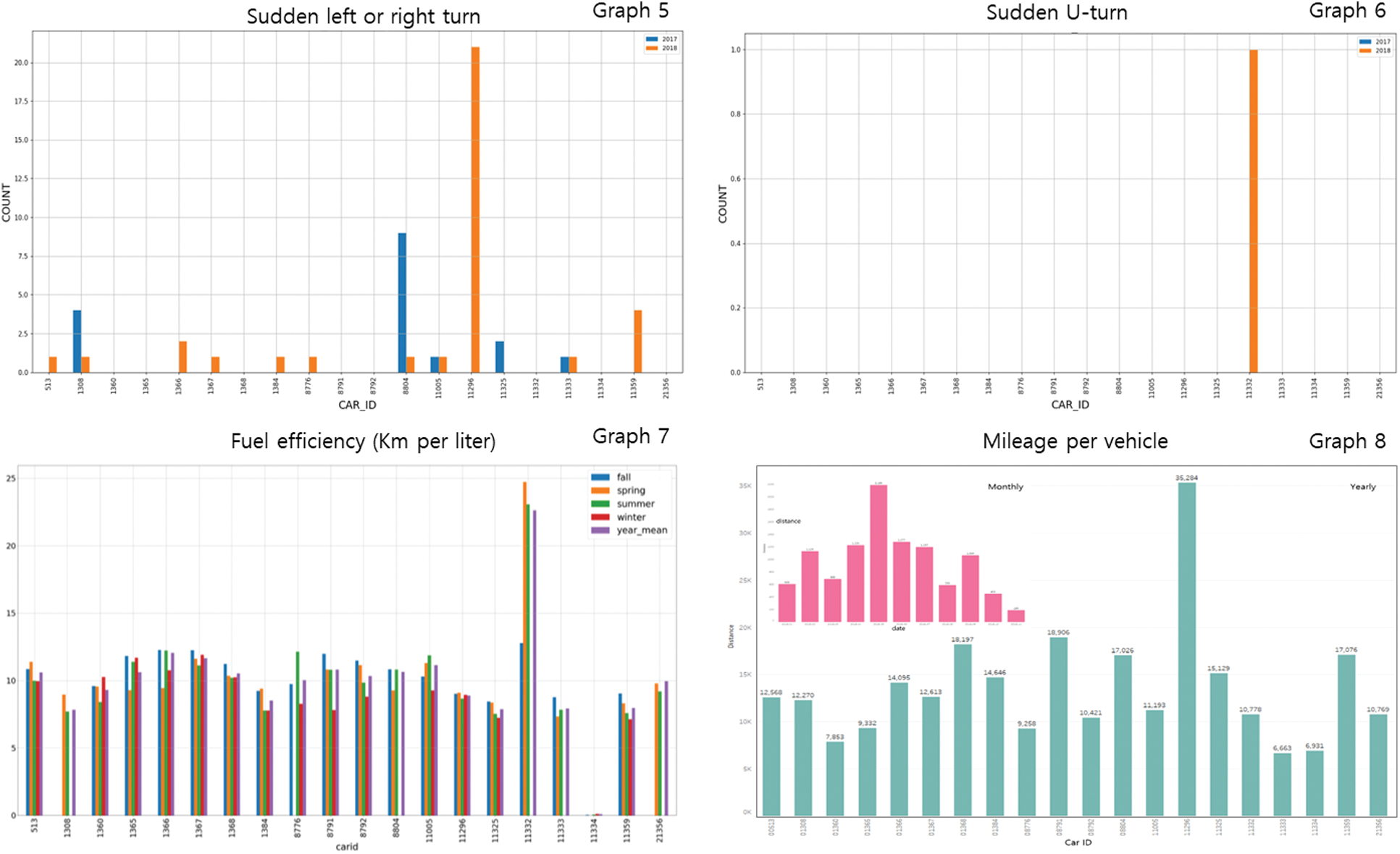
Figure 8: Driving behavior patterns

We also applied the analysis module we developed earlier based on the data received from Company C to the vehicle data of a second company (Company B). The module was used to identify dangerous driving patterns based on the data of Company B.

We analyzed all the data for January 2020 and the results are shown in Fig. 9, where the x- and y-axes represent the vehicle number and the number of counts for each pattern, respectively. Fig. 9 (graph1) shows the rapid acceleration pattern of vehicles of Company B. The results show that, with the exception of vehicle 11, most vehicles did not perform a large number of rapid accelerations. In addition, graph2 in Fig. 9 shows the results for the rapid deceleration pattern and shows that the number of rapid decelerations of vehicle 11 was the highest. Fig. 9 (graph3 and graph4) shows the quick start and sudden stop patterns. The results of this analysis also show that most of the vehicles except for vehicle 11 did not perform a large number of rapid accelerations, quick starts, or sudden stop patterns.

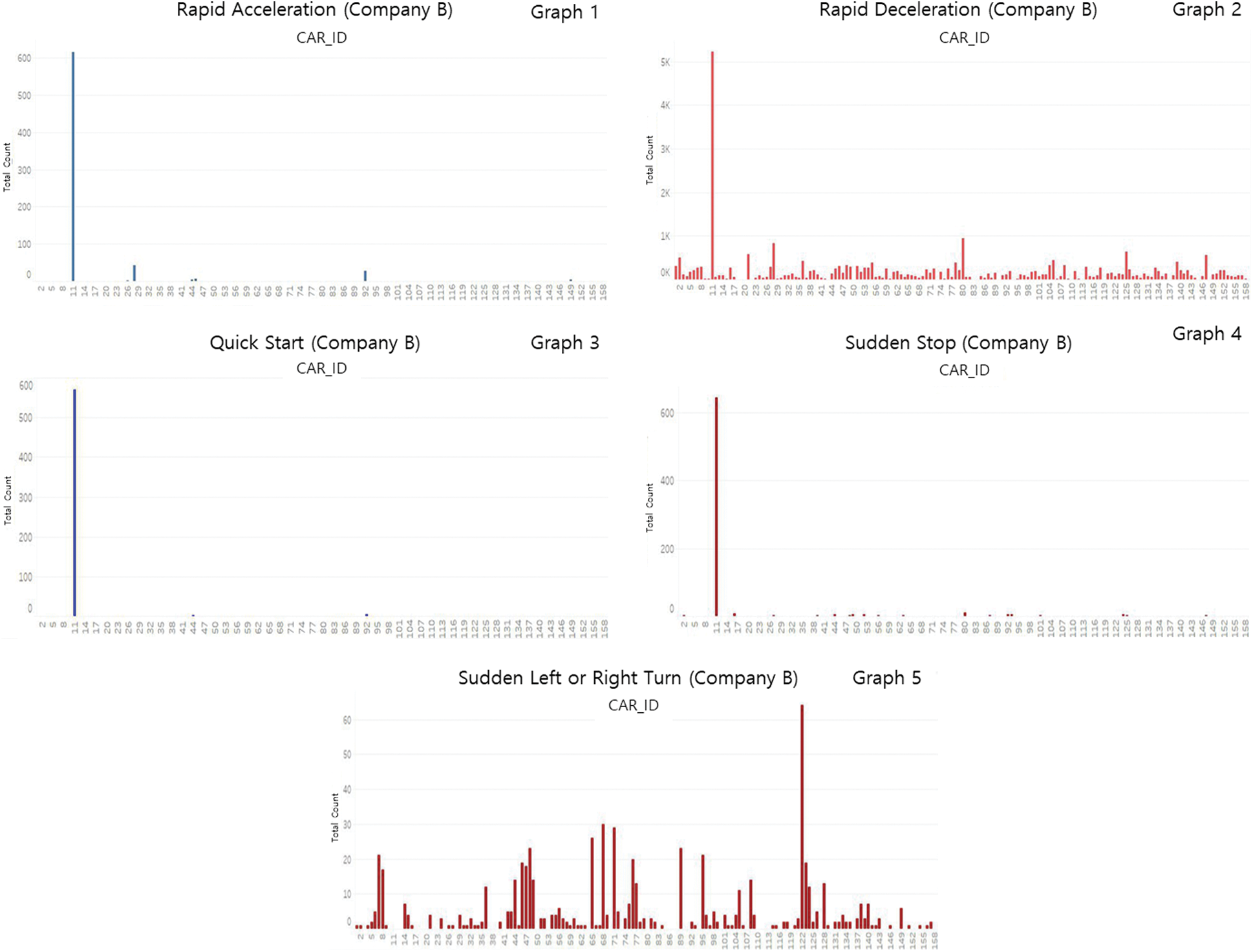
Figure 9: Driving behavior patterns (Company B)

The results of the data analysis of Company B are summarized as follows. As shown in the previous analysis (Company C), a vehicle generally decelerates more frequently than accelerating rapidly. The difference from the previous data analysis is that the number of rapid acceleration and deceleration patterns was significantly higher for vehicle 11. This is expected because the data were collected from logistics vehicles. In other words, quick start or sudden stop would not be expected to occur frequently compared with a general passenger car in the case of a logistics vehicle operated by an experienced driver compared to a general passenger car driven by a layman. In addition, the drivers of logistics vehicles would be unlikely to accelerate repeatedly because they drive considering the fuel efficiency of the vehicle. The results of the sudden left or right turn analysis are shown in graph5 in Fig. 9, which shows that the pattern of sudden left or right turns is evenly distributed throughout the vehicles. The largest number of sudden left or right turns during one month was performed by vehicle 122, which performed more than 60 in a month. Conversely, vehicle 11 did not exhibit a pattern of sudden left and right turns despite having the highest number of rapid accelerations, rapid decelerations, quick starts, and sudden stops (as of January 2020). A pattern of sudden U-turns could not be identified from the analysis of the data of this company (as of January 2020).

We also analyzed the trajectory of a vehicle using GPS data and DBSCAN. For each point in a cluster, the algorithm requires the existence of at least a minimum number of points (MinPts) in an Eps-neighborhood of that point. The formula is defined as follows [10]:

Here, the Eps-neighborhood of a point p, denoted by (p), and point A is directly reachable from p if point q is within distance epsilon () from core point p, where epsilon () denotes the distance to define the neighborhood. The purpose of trajectory analysis is to analyze the driving route and main operating locations of vehicles. Before performing the trajectory analysis, we derived the main locations of the vehicle based on the GPS data, and clustered the collected data using the DBSCAN algorithm based on the derived main locations. Because GPS data are not received when the vehicle is turned off, the main location of the vehicle is derived by using two rules according to the operating conditions of the vehicle. The method for deriving the main location of the vehicle is as follows. First, GPS data are continuously collected while the vehicle is in operation. Therefore, we defined the location as the main driving (operating) location when GPS data from the same location were received for more than 5 min (when the vehicle is turned on). Second, GPS data are not continuously collected while the vehicle is turned off. Therefore, when the GPS values received when the vehicle stops and when the vehicle is turned on after some time are within the same range, this location is defined as the main driving (operating) location. We performed cluster analysis of data collected from 315 vehicles of Company A based on the DBSCAN algorithm and the major driving (operating) locations (visited points) we derived. We analyzed the main driving (operating) location of the vehicle in detail by adjusting the values of epsilon () and MinPts which is the minimum number of neighbors within epsilon () radius, and clustered the main driving (operating) locations into 11 groups. Based on the map, of the 11 clustered groups, five clusters were concrete batch plants (Factories A–E), and two clusters were garages where the vehicles were parked. The locations of the remaining four clustered groups were unspecified, and these locations were identified as concrete placement points within the construction site. Fig. 10 (Map A) shows the driving route of a vehicle on a map, based on the Folium library. Analysis of the data revealed that the driving ranges of many vehicles were identical. In addition, most of the vehicles were operated in the driving section within 1 h 30 min (1.5 h), as shown in Fig. 10 on the right (Map B).

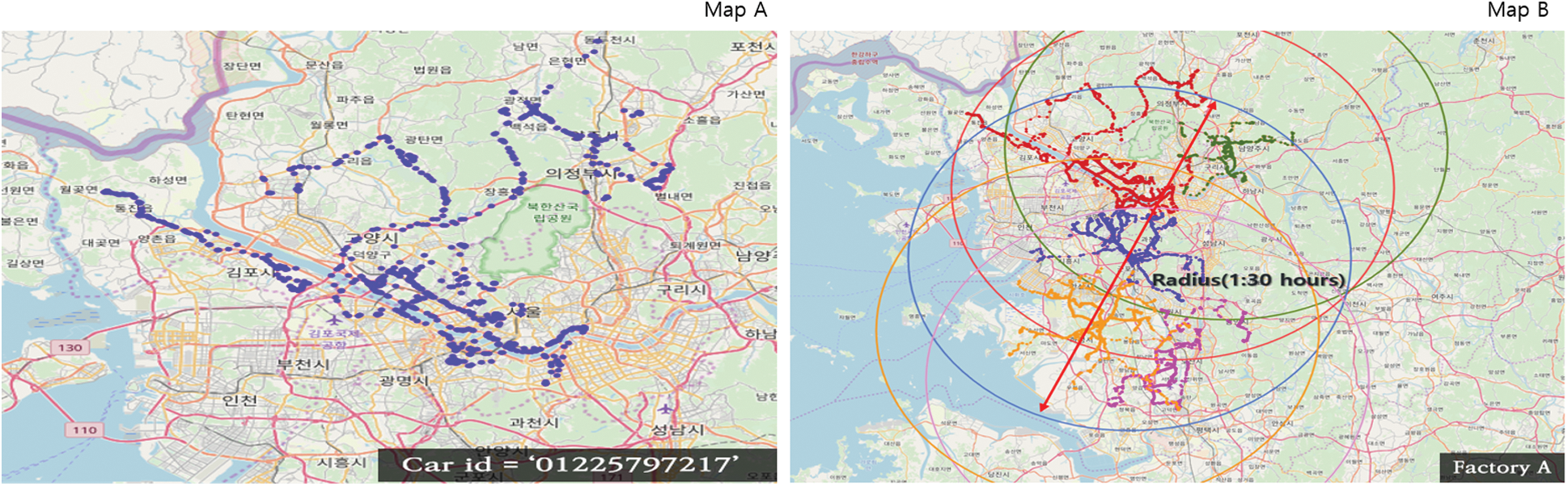
Figure 10: Vehicle route and driving radii of vehicles

We analyzed and predicted the time-series data using the ARIMA and LSTM models in this study. Parameters such as the battery voltage (BATTERY_VOLTAGE), coolant temperature (COOLANT_TEMPER), and engine oil temperature (ENGINE_OIL_TEMPER) of the vehicle were used for analysis and prediction.

The data used for the prediction and analysis were collected from one vehicle of Company B for 2 h (from April 15, 2020, at 22:10 to April 16, 2020, at 00:09:59). Because data were collected every second, 7200 data (rows) were collected per parameter. The analysis and results for the prediction of the battery voltage data are described here. Fig. 11 (Graph A–C) shows the results that were obtained using the ARIMA model. In this graph, the x-axis contains the time axis in seconds and the y-axis represents the battery voltage (26.0 V up to 29 V). The orange and blue lines represent the actual and predicted battery values, respectively. In addition, graph (A) in Fig. 11 shows the actual and predicted battery voltage for the first 10 min. Here, we can see that the voltage decreased from the beginning of the vehicle operation to approximately 4 min, where after it stabilized at 28 V. Graph (B) in Fig. 11 shows the actual and predicted values for the last 10 min of driving. Fig. 11 (graph (C)) shows the actual and predicted battery voltage for the last 5 min (after 1 h 55 min), and the gray area in the graph shows the predicted battery voltage (blue line) for 1 min after 2 h. As shown at the top (Graph A–C) of Fig. 11, the prediction model that was implemented seems to be correct, with the predicted values being in good correspondence with the actual values. In fact, the battery voltage predicted for the last 10 s (after 1 h 59 min 50 s) was 28.37 V and the actual value was 28.4 V, indicative of very high prediction accuracy. The maximum value of the actual battery voltage for 10 s was 28.7 V, and the minimum value was 28.3 V. We fitted the model without constraints (); the detailed information of the model is shown at the bottom (D) of Fig. 11. The prediction results of the coolant temperature and engine oil temperature using the ARIMA model were also highly accurate.

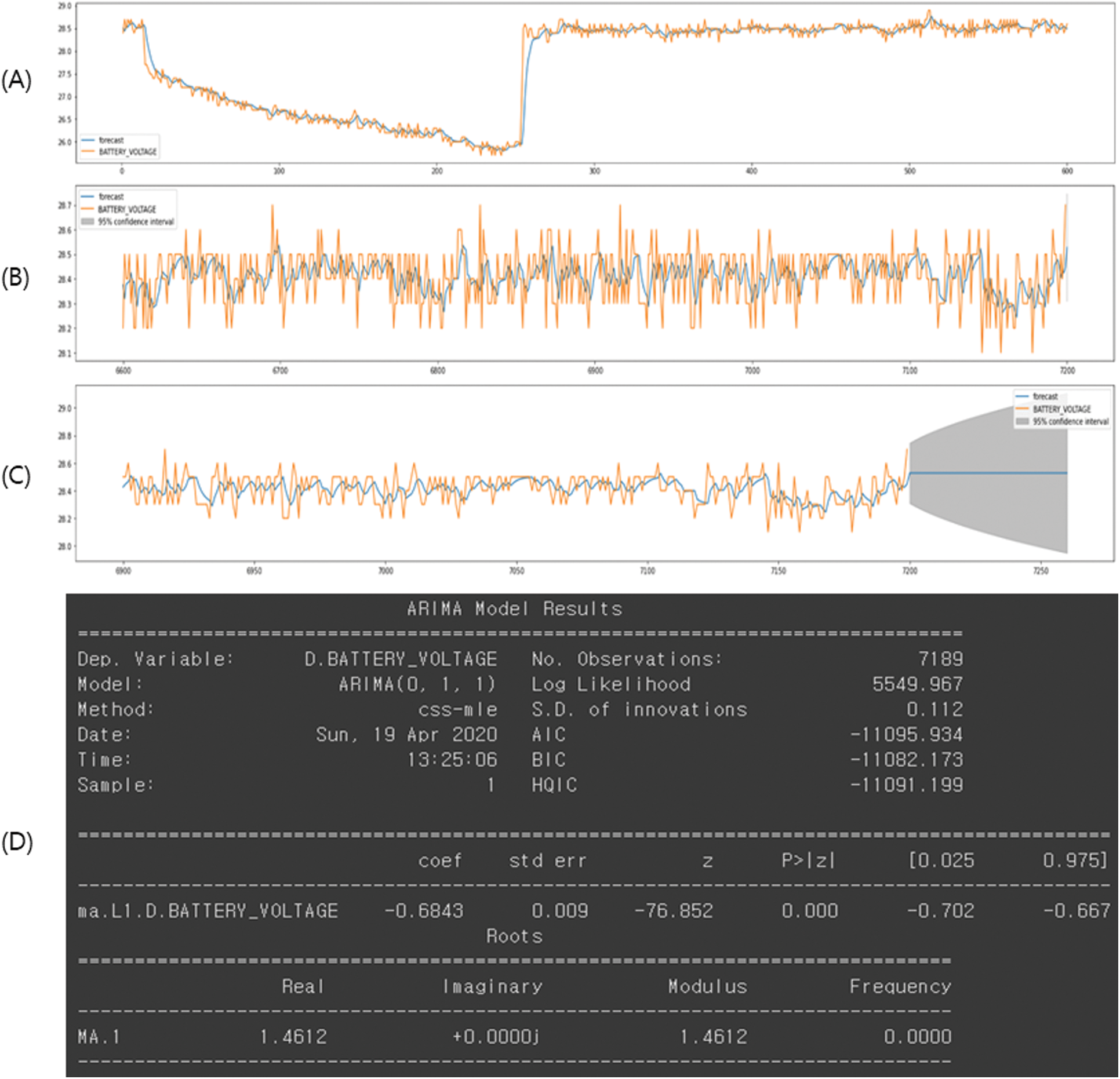
Figure 11: Prediction of time-series data using ARIMA (battery voltage)

Next, we used the LSTM model, in this case a stateful stacked model, to estimate the battery voltage, coolant temperature, and engine oil temperatures. The data are composed of 7200 data points for 2 h, as in the ARIMA model; the data structure for training the model is as follows. We trained the model using 3600 data points (1 h) and evaluated our model using data from 30 min (1 h to 1 h 30 min). The testing was conducted with the data of the remaining 30 min (1 h 30 min to 2 h). The battery voltage data were scaled using the MinMaxScaler class (maximum value 1, minimum value 0), and the loss function was set to “mean_squared_error.” Adam, which is an adaptive learning rate optimization algorithm that was designed specifically for training deep neural networks, was also used as the optimizer [24]. The estimated value of the battery voltage based on LSTM is shown in Fig. 12, in which the x- and y-axes represent time (s) and the value obtained by scaling the battery voltage data of the vehicle (Max 1, Min 0) respectively. The predicted value in the graph, the red line with the value of 0.850, is equal to 28.42 V. That is, the predicted value of the battery voltage of the vehicle using the LSTM model is 28.42 V. Considering that the average battery voltage of the data collected for 2 h is 28.39 V, the predicted value is considered to be fairly accurate (99.89% of average values). However, it does not appear to follow the trend shown in the graph (red line) in Fig. 12. In addition, the values predicted for the temperatures of the coolant and engine oil using LSTM were inaccurate. Currently, we are conducting research to find and create models to overcome these problems.

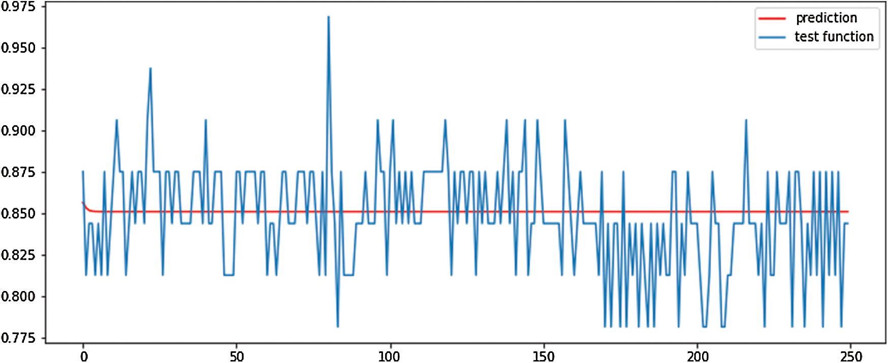
Figure 12: Prediction of time-series data using LSTM (battery voltage)

5  Conclusions and Future Work

In this paper, we extensively described our big data analysis platform, the structure of data collection, the development environment of the analysis software, data processing procedures, and the structure of the data analysis software including preprocessing. We performed various analyses, such as correlation, rapid acceleration and rapid deceleration, quick start, sudden stop, sudden left turn, sudden right turn, sudden U-turn (dangerous driving patterns), mileage, fuel efficiency, and trajectory analysis based on the analysis software we developed. In addition, ARIMA and LSTM models were used to predict vehicle data, such as the battery voltage. A summary of the representative results is as follows: Most vehicles had unique driving patterns, such as rapid acceleration and deceleration, and sudden stop and start. In fact, a vehicle with a large number of rapid accelerations has a high number of rapid decelerations according to our analysis. The fuel efficiency was generally higher in summer than in winter. Moreover, most of the vehicles belonging to one company had similar driving radii in the trajectory analysis. Currently, we are working on expanding our analysis software; we are conducting research to develop new business models based on the software we developed and the results of our analyses. In particular, we are analyzing the driving patterns of automobiles efficiently by improving the performance of the trajectory analysis algorithm. In future, we aim to identify ways in which to apply deep learning and machine learning algorithms, such as decision trees, SVMs, and LSTM, to automotive data using a variety of approaches. Furthermore, we plan to conduct research on the analysis of unstructured data, such as vehicle-related images and video files, based on artificial intelligence technology. Eventually, we expect to derive more accurate analysis results and create various business models based on the analyzed results.

Funding Statement: This work was supported by the Technology Innovation Program (10083633, Development on Big Data Analysis Technology and Business Service for Connected Vehicles) funded by the Ministry of Trade, Industry & Energy (MOTIE, Korea).

Conflicts of Interest: The authors declare that they have no conflicts of interest to report regarding the present study.

This work is licensed under a Creative Commons Attribution 4.0 International License, which permits unrestricted use, distribution, and reproduction in any medium, provided the original work is properly cited.