DOI:10.32604/cmc.2021.014983
| Computers, Materials & Continua DOI:10.32604/cmc.2021.014983 | |
| Article |
Multiclass Stomach Diseases Classification Using Deep Learning Features Optimization
1Department of Computer Science, HITEC University, Taxila, 47040, Pakistan
2College of Computer Science and Engineering, University of Ha’il, Ha’il, Saudi Arabia
3Department of Informatics, University of Leicester, Leicester, UK
4Department of Mathematics and Computer Science, Faculty of Science, Beirut Arab University, Lebanon
5Department of Computer Science and Engineering, Soonchunhyang University, Asan, Korea
*Corresponding Author: Yunyoung Nam. Email: ynam@sch.ac.kr
Received: 31 October 2020; Accepted: 16 December 2020
Abstract: In the area of medical image processing, stomach cancer is one of the most important cancers which need to be diagnose at the early stage. In this paper, an optimized deep learning method is presented for multiple stomach disease classification. The proposed method work in few important steps—preprocessing using the fusion of filtering images along with Ant Colony Optimization (ACO), deep transfer learning-based features extraction, optimization of deep extracted features using nature-inspired algorithms, and finally fusion of optimal vectors and classification using Multi-Layered Perceptron Neural Network (MLNN). In the feature extraction step, pre-trained Inception V3 is utilized and retrained on selected stomach infection classes using the deep transfer learning step. Later on, the activation function is applied to Global Average Pool (GAP) for feature extraction. However, the extracted features are optimized through two different nature-inspired algorithms—Particle Swarm Optimization (PSO) with dynamic fitness function and Crow Search Algorithm (CSA). Hence, both methods’ output is fused by a maximal value approach and classified the fused feature vector by MLNN. Two datasets are used to evaluate the proposed method—CUI WahStomach Diseases and Combined dataset and achieved an average accuracy of 99.5%. The comparison with existing techniques, it is shown that the proposed method shows significant performance.
Keywords: Stomach infections; deep features; features optimization; fusion; classification
Gastrointestinal tract (GIT) infections identification is an active research area in medical image processing [1]. The primary GIT infections are polyp, bleeding, ulcer, and esophagitis [2]. According to the American Cancer Society (ACS), mostly older people are affected by stomach infections and cancer. They are primarily an average age of 68 years. In America, since 2020, 27,600 peoples are affected due to stomach cancer, and from them, 11,010 peoples are died [3]. The risk factor of stomach cancer is higher in men as compared to women. From the last ten years, stomach infections are decreasing by up to 1.5% [4]. Wireless Capsule Endoscopy (WCE) is the latest technology in medical imaging [5]. It has low risk as compared to Capsule Endoscopy (CE) [6]. It is considered a first-line examination tool in the clinics for stomach abnormalities like ulcers, polyps, etc. Usually, it is an 8 min examination of one patient.
For 8 min examination, approximately 56,000 frames are generated. But from them, only a few frames are important, and the rest of them is discarded. However, this selection of important frames is an essential task because, from 56,000 frames, it is not easy to identify infected structures [7]. The experts perform this task manually, which is hectic and time-consuming. After selecting important frames, another study is to classify the frames according to infections like polyp, ulcer, bleeding, etc. A highly expert person is always required for manual labeling of this task. Therefore, an automated computerized system is necessary to identify these infections without helping any expert by using WCE frames [8]. But issues like low contrast and complex background are facing by such systems for accurate identification.
In recent years, many computerized techniques are presented for medical disease detection and classification. They focused on well-known medical imaging modalities such as mammography for breast cancer [9], pathology [10], Electroencephalogram Signals [11], carcinoma [12] such as deep learning (DL) shows much improvement in medical image processing [13,14]. DL is a powerful machine learning tool for automated medical infections classification into their relevant category [15,16]. It can improve the abilities and health professionals in the context of early identification of these diseases. Convolutional Neural Network (CNN) is a major form of deep learning for extracting deep high-level features against one image. CNN can process input data into various forms like images, signals, multi-dimensional, and videos. A simple CNN model consists of several layers like convolutional, pooling, fully connected (FC), and classification [17]. The low-level features are extracted from the initial layers and going deeper for the extraction of high-level features. In the FC layer, features are vectorize for final classification. The most used pre-trained CNN models are AlexNet [18], VGG [19], ResNet [20], and GoogleNet [21]. These models are trained on the ImageNet dataset [22] and later utilized by many researchers for medical imaging with transfer learning.
According to the previous study [23], it is observed that the optimization of the most optimal features is more useful for accurate classification of stomach infections. The primary purpose of feature optimization is to improve a system’s accuracy and minimize a system’s time during the features learning [24]. This article attempts to resolve high computational time and improved accuracy for the classification of stomach infections. Moreover, few other problems are also considered, such as redundancy among extracted features, the presence of irrelevant features that are not required for final classification, and degrade the accuracy of stomach disease classification. We followed the features optimization problem by employing metaheuristic algorithms and fused their performance for final classification. For classification, Neural Network is the most active supervised learning method and utilized for final features classification. Our major contributions in this work are given as follows:
Ant Colony Optimization (ACO) for pixel intensity value improvement is applied to fuse two filters’ output.
Retrain Inception V3 deep learning model using transfer learning and extract high-level features from Global Average Pool (GAP) layer.
Deep features are optimized using the Crow search algorithm and PSO along with dynamic fitness function. The maximal approach fuses the resultant optimal features.
Multilayer perceptron neural network (MLNN) is implemented for the classification of optimal fused features. A fair comparison is also conducting with contemporary techniques based on accuracy and time (testing time).
The rest of the paper is organized as follows: related work is presented in Section 2. The proposed method, which includes features optimization, fusion, and MLNN based classification, is described in Section 3. Results and discussion are presented in Section 4, and Section 5 concludes the paper.
In medical imaging, several deep learning techniques are implemented in the past two years and showed considerable success. For stomach diseases, deep learning models [25] were utilized to enhance classification accuracy. The Kvasir dataset was trained on the deep networks, including Inception-v4, NASNet, and Inception-ResNet-v2. In [26], ResNet50 deep model was utilized to classify the bleeding and healthy WCE images. This model achieved a sensitivity of 96.63%. Khan et al. [14], developed a CAD system for the classification of stomach diseases. The researchers implemented the active contour segmentation on HSI color space, and then a novel saliency method was applied to the YIQ color space. They evaluate this method on their private dataset, consisting of 9000 bleeding, ulcer, and healthy images. The average segmentation accuracy achieved is 87.9635% for ulcers, and the classification results are very promising. A model [27], was presented based on the handcrafted and convolutional neural network (CNN) features. Gabor features and DenseNet based Faster Region-Based CNN (Faster R-CNN) were combined to detect the abnormal regions in the esophagus from WCE images. They evaluate their method on the Kvasir and the MICCAI 2015 dataset and achieve the precision of 92.1% and 91% respectively.
A deep learning-based model [28] was presented for the detection of stomach diseases. They proposed the Mask Recurrent CNN (RCNN) model for the segmentation of the ulcer region. In the classification phase, transfer learning is applied to ResNet101 for the deep feature extraction. This model achieved 99.13% classification accuracy on the cubic SVM classifier. In [29], the transfer learning approach was utilized to classify normal, benign ulcers, and cancer. Transfer learning was done using VGGNet, Inception, and ResNet. The highest performance was achieved on the ResNet model. A system [16] was developed based on the DenseNet CNN (DCNN) model to recognize stomach abnormalities. In this model, color features were extracted from the HSV and LAB color spaces, and DenseNet features were extracted by applying transfer learning.
In the feature selection step, Tsallis entropy is implemented for the selection of robust features. A method [8] was developed to classify stomach infections based on the handcrafted and deep features. Color, Discrete Cosine Transform (DCT), Discrete Wavelet Transform (DWT), and deep VGG-16 features fused, and selection of features done through Genetic Algorithm (GA). A novel preprocessing technique [30] was proposed to enhance the classification accuracy to recognize normal and bleeding regions. Zhao et al. [31] designed a rotation-tolerant image feature. This novel feature is rotation invariant and showed its effectiveness in the detection of stomach abnormalities. This technique, with only 126 image features, performed better as compared to the HOG features. A-scale technique was proposed based on completed local binary patterns and Laplacian pyramid (MS-CLBP) [32] to identify ulcer regions. The ulcer’s detection was done using the Green component from RGB color space and Cr component from the YCbCr color space. This proposed method achieved an average accuracy of 95.11% on the SVM classifier. A deep learning-based model [33] was developed for the classification of abnormal and normal frames. This method utilized a Weakly Supervised Convolutional Neural Network (WCNN) for classification. A Deep Saliency Detection (DSD) method was used for detection, and an Iterative Cluster Unification (ICU) method was used to localize the anomalies. The highest AUC achieved by this method is 96%.
A CAD system [34] was proposed based on the fusion of geometric and deep CNN features to classify WCE images. The geometric features were extracted from the segmented image and fused with VGG-16 and VGG-19 deep features. Euclidean Fisher Vector method was utilized for the fusion of features, and the best features were selected using the conditional entropy technique. The selected feature set finally fed to the K-Nearest Neighbor (KNN) for classification. A super-pixel segmentation method [35] was proposed to detect bleeding areas in WCE video frames. The CMYK color space helped to segment the bleeding region more accurately. The above studies show that the deep learning models give improved accuracy; however, it is also noted that the researchers are facing problem in the selection of good features for final classification. Therefore, we are considering the problem of best features using the optimized features fusion.
In summary, the numerous existing techniques used deep learning models for the classification of stomach infections. Few of them combined deep models and achieved better accuracy, but computational time is significantly increased. In the few studies, the contrast of original images is improved and then trained a deep learning model. They also applied feature selection techniques to select the best features for better classification accuracy.
An automated optimized deep features based design is presented to classify stomach diseases using WCE images. The proposed method consists of a few important steps, as illustrated in Fig. 1. First, the contrast of original images is improved and utilized to train the pre-trained CNN model—Inception V3. Extracted deep learning features are optimized using two metaheuristic techniques—PSO and dynamic fitness function and Crow search algorithm. After that, the optimal features are selected from the original search space and fused through the maximal fusion approach. Final features are classified using MLNN and in the output return—labeled images and numerical results.
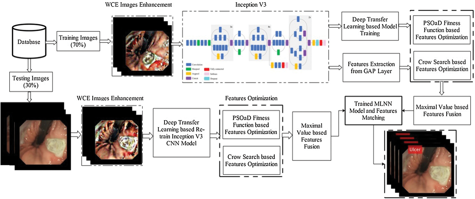
Figure 1: The proposed architecture of stomach disease classification using optimized deep learning features
Enhancement of contrast in an image is an important step and essential for better visualization of an object in the image. This step’s main advantage is to get stronger and more relevant features for the accurate classification of medical infections. In this article, we presented a hybrid contrast enhancement approach for WCE image improvement. Initially, fused the output of two filters named—top-hat and bottom-hat and then applied the ACO algorithm for pixel enhancement. Mathematically, the complete enhancement process is defined below:
Consider, we have WCE images datasets  and one image is denoted by
  of dimension
  . It is not an original size, but we resize database images according to this dimension. Let,
  denotes resultant top-hat filtering image,
  denotes bottom-hat filtering image, and
  denotes a fused image of the same dimension as input. The top-hat and bottom hat filters are defined as follows:

where,  represent the opening operator, b denotes the structuring element, and its value is defined as 20.

Here,  represent closing operator, and b is the same as structuring element. Later, fused the output of both images using the following equations:


where,  represent the output of the original and top-hat image and
  describe the addition operation.
  is a fused filtered image and
  represent subtraction operation, respectively. This operation subtracts the image obtained by Eq. (3) and the image obtained by Eq. (2). The size of this fused image same as the input image
  . The visible results of this step are showing in Fig. 2 (second row). After this, we applied ACO further to increase the pixel intensity level. ACO is a metaheuristic algorithm [36] and recently been involved in many applications for different purposes. The idea of ACO is indirect communication among folks of a generated population. In this algorithm, ants are following the shortest path between their nest and food source. Three main steps are involved in this algorithm—initialization, pheromone update, and final solution. Initially, set the upper limit of pheromone. Then in the solution phase, each ant is randomly selecting a vertex. Each ant selects the next vertex based on the Roulette approach, which is based on probability. This process is continuing until the complete path is completed. Mathematically, it is defined as follows:

where,  denotes starting and ending points, quv denotes pheromone factor, wuv represent heuristic factor, set of nodes are represented by
  , and
, and  represent heuristic factor, respectively. The next step is to update the pheromone process for the enhancement of the solution. The updating process is defined as follows:

where, e represent evaporation parameter of range  and total pheromone amount define by
  of kth optimal path. The optimal solution in each path selected as follows:

where the current optimal solution set is defined by Cos. Hence, for final fitness function if f(C) < f(Cos), then pixels are updated as the current optimal solution and continuing until all iterations are completed. After all iterations, we obtained a new image in which all optimal pixels are move to the infected part. Visually, results are illustrated in Fig. 2 (third row).
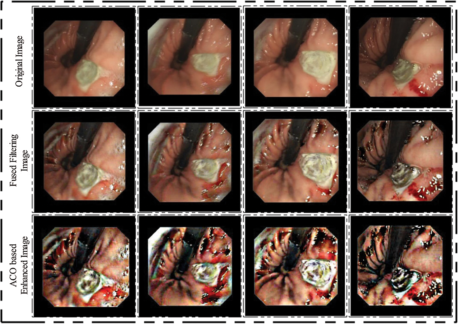
Figure 2: Hybrid WCE images enhancement results
3.2 Deep Learning Features Extraction
Inception V3: Inception V3 is a directed acyclic graph (DAG) network with 350 connections and 316 layers, including 94 convolutional layers [37]. The DAG network structure expresses the complex system of a network having multiple inputs to multiple layers. Numerous filters are applied on many layers of this network for feature extraction. The flexibility of inception V3 allows for applied different sizes of filters and parameters on the same layer than the traditional CNN layer with fixed parameters. Initially, the Inception V3 is trained on challenging and largest image database ImageNet [22], having 1000 classes and over a million images. The network has learned a wide range of various features of different objects. The input size of the image for the inception V3 is 299-by-299-by-3. This article uses this model for the classification of stomach infections like ulcers, polyp, etc. For training of this model on the stomach database, the deep transfer learning concept is applied.
Deep Transfer Learning: Transfer learning is a widely adopted technique for recognition and detection tasks. The pre-trained models are used to enhance the performance of machine learning tasks. Transfer learning [38] can be defined as the domain D with two components: a feature vector  and a probabilistic distribution P(Y); can be defined as
  and we have a task having T with two components one is ground truth
  and second is objection function
  . This function can be trained using a training database. f(.) function is utilized to predict the class label f(y) of an unknown class label y. The function can be written as in probabilistic form as
  . Transfer learning can be expressed in terms of domain source like as
  and learning rate ST and the targeted output can be expressed as
  and the targeted function will be illustrated as SS. Transfer learning major target is to enhance the learning rate for the prediction of the targeted object using the recognition function fS(.) based on the training for learning from BT and BS, where
  and
and  . Inductive transfer learning is efficient in pattern recognition. An Annotated database is required for efficient training and testing while implementing inductive transfer learning. Transfer learning can be performed using different class labels
  and differential distributions
  . The distribution function of image P(YT) can be eliminated by on the last layer using function fT(.) which is used for new label prediction by removing linear function for new label prediction SS using function fS(.). Transfer learning is efficient in dealing with fewer amounts of data in medical imaging field. The middle layers of deep CNN models, while performing transfer learning, can be utilized as an input feature space for classifier training while dealing with different tasks to improve the recognition performance [39]. The adopted deep transfer learning (TL) model is expressed in Fig. 3. In the learning process through TL, initialized the learning rate of 0.0001 and mini-batch size of 28. The activation function is applied on the global average pool (GAP) layer and obtained a resultant feature vector of dimension
  .
.
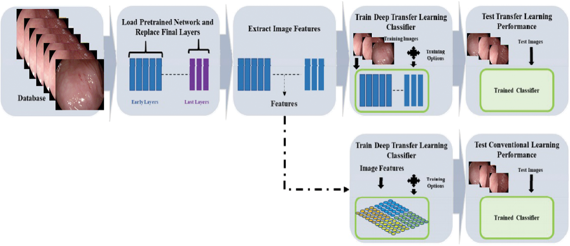
Figure 3: Process of the deep transfer learning model
Features optimization is an essential step for selecting the most optimal features by employing Metaheuristic techniques. The main aim of this step is to neglect the irrelevant features from the final classification step. In this article, two optimization techniques are implemented: i) Crow Search Algorithm (CSA) and ii) PSO along with Dynamic Fitness Function. Visually, the process of this step is shown in Fig. 4. In this figure, it is illustrated that the original feature vector of dimension  is feed in the optimization algorithms. In in the output, two optimal vectors are obtained of dimension
  and
and  , respectively. It is noted that this resultant vector size has been changed according to the nature and size of datasets. The detailed mathematical description of each method is given below.
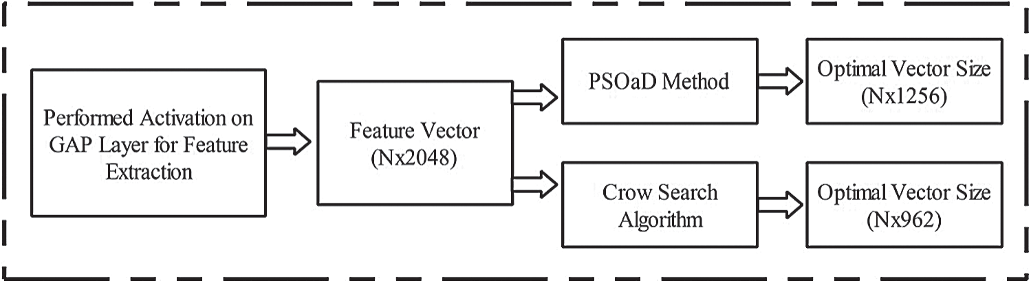
Figure 4: Flow diagram of deep features optimization
The Crow Search Algorithm (CSA) [40] is a metaheuristic optimization method. CSA is a population-based approach that is inspired by the intelligent behavior of crows. This approach works based on the idea that crows store their extra food and utilized it when needed. The orientation of each crow i at the generation gtn can be represented by a vector  . The possible solutions are given as:

where N is the number of populations, the maximum number of generations is gtnmax.The memory  represents the hiding position of food of each crow, and this is observed as the best position. After each generation, each crow moved to a new location. This new location is mathematically described in the following equation:

where,  denotes the flight length of ith crow,
  represents the awareness probability of jth crow at generation gtn, Ri and cj are the random numbers, and
  represents the memory of jth crow. The value
  significantly influence the algorithm. The higher values of flight length help global search problems and lower local search values [41]. Initially, each crow is randomly placed in the search space. It is considered in this step that its initial positions represent the memory of the crow. The new position of crow is evaluated during each generation by utilizing a fitness function fn, and the memory position of crow is updated according to the following equation:

After this, positions are updated until all iterations are performed and obtained an optimal vector of dimension  . This vector’s length is not consistent and may be changed according to the input and defined problem.
3.3.2 Particle Swarm Optimization (PSO)
PSO is a biologically inspired algorithm derived from the swarm’s social behavior for its survival [42,43]. This algorithm’s main objective is to find the best possible solution for the problem from a given set of solutions. A swarm refers to the set of candidate solutions, and each solution is a particle. Each particle has its specific position and moves with some velocity in the search space. After each iteration, the PSO obtains the best solution, and the position is changed. The particle selects the new position based on previous knowledge [44]. Each particle is evaluated according to the defined fitness function. In the end, PSO finds an optimal solution.
Suppose there is an N-dimensional search space with n number of particles, the N-dimensional vector for the ith particle of the swarm is denoted by  . The previous best location of the ith particle is
  , this gives the best fitness value. The lowest function value particle is represented as
  . The velocity of the ith particle is represented as
  . The manipulation of particles is done according to the following equations:


where  represents the inertia weight, rand(), and Rand() are random functions that generate the pseudorandom values within the range [0, 1]. z1 and z2 are the two constant positive numbers cognitive parameter, and social parameter, respectively.
In the first equation, the velocity of ith particle is calculated at each iteration.  calculates the distance between the ith particle and its personal best location.
  calculates the distance between the ith particle and global best location. The functions
  and
and  makes the algorithm more flexible because these functions provide randomness [45]. In the second equation, the new position of ith particle is calculated. The multi-layered neural network (MLNN) is employed as a fitness function and accuracy measure is used for the analysis. Based on the fitness function, the best particles are analyzed, but we have a problem with the number of iterations. Therefore, we update the fitness function with dynamic change. In the dynamic change, iterations are stopped when the accuracy of MLNN is decreased up to 4 iterations and consider the last highest accuracy. In this work, by following this approach, we obtained an optimal feature vector of dimension
  after 21st iterations.
3.4 Features Fusion and Classification
Finally, obtained optimal features are fused in one vector by a new equation based on maximal value. Feature fusion aims to improve the accuracy performance of the proposed algorithm. However, on the other side, it has one major disadvantage—prediction and training time are increased. Consider, we have two feature vectors  and
and  , where X1 denotes feature vector of CSA of dimension
  and X2 denotes feature vector of PSOaD of dimension
  , respectively, then the fused vector is defined as follows:

where,  is output fused feature vector and X3 is output after each iteration. The total number of iterations is performed based on both vectors’ total dimension length, such as
  . Hence, we obtained a final feature vector after fusion of dimension
  . Of the total, 252 features are irrelevant, which are removed during the final fusion. Finally, we implemented a multilayer perceptron neural network (MLNN) for the final features classification [46]. An MLNN consists of an input layer followed by a hidden layer and output layer. The fused features are considered as neurons; then output is generated as follows:

where,  is the output of this network, Wj represent weight values, and
  represent hidden layers, respectively. There is no hard rule for selecting optimal neurons, so we choose input units to be 600 having one hidden layer and 50 neurons. Bayesian backpropagation is applied to achieve the best accuracy. In the output, numerical values and labeled results are obtained. A few labeled results are showing in Fig. 5.
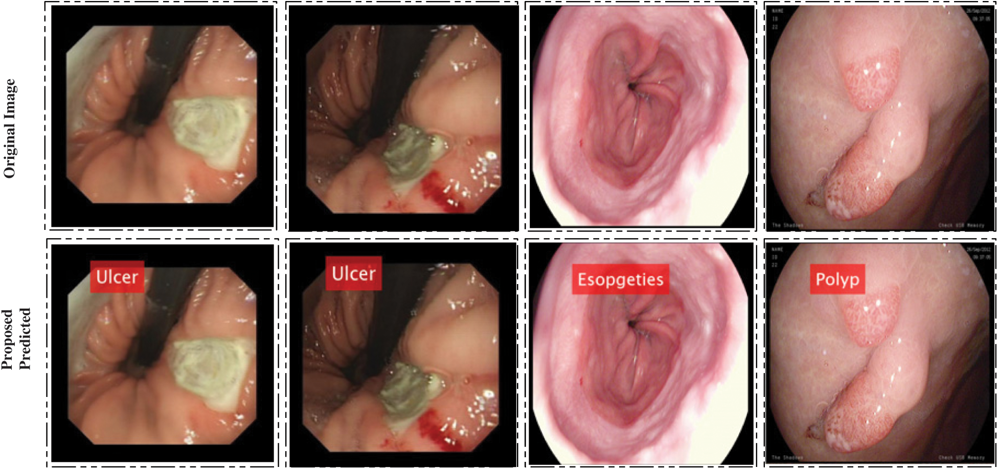
Figure 5: Proposed system prediction results
4 Experimental Setup and Results
The proposed technique was evaluated on combined publicly available datasets. The dataset contains 15,000 color images of different stomach infections. Stomach bleeding and healthy image classes are obtained from [14] having 3000RGB images per class. Ulcerative-colitis and esophagitis classes extracted from publicly available stomach disease dataset Kvasir [47]. Data augmentation was performed to increase the images per category. The polyp class of dataset was acquired from Kvasir [47], ETIS-LaribPolypDB [48], and CVC-ClinicDB [49]. A 70:30 approach is employed during the learning of the proposed model, where cross-validation was 10-fold. Multiple classifiers are selected for a fair comparison of MLNN. The other chosen classifiers are a fine tree, linear discriminant, Naïve Bayes, and ensemble classifier. Each classifier’s robustness is evaluated using multiple performance evaluation measures like accuracy, precision, sensitivity, F1 Score, and computational time. All experiments are carried out using Intel Core i7, an 8th generation CPU equipped with 16 GB of RAM and 8 GB GPU. For a tool, the MATLAB 2019a version was used.
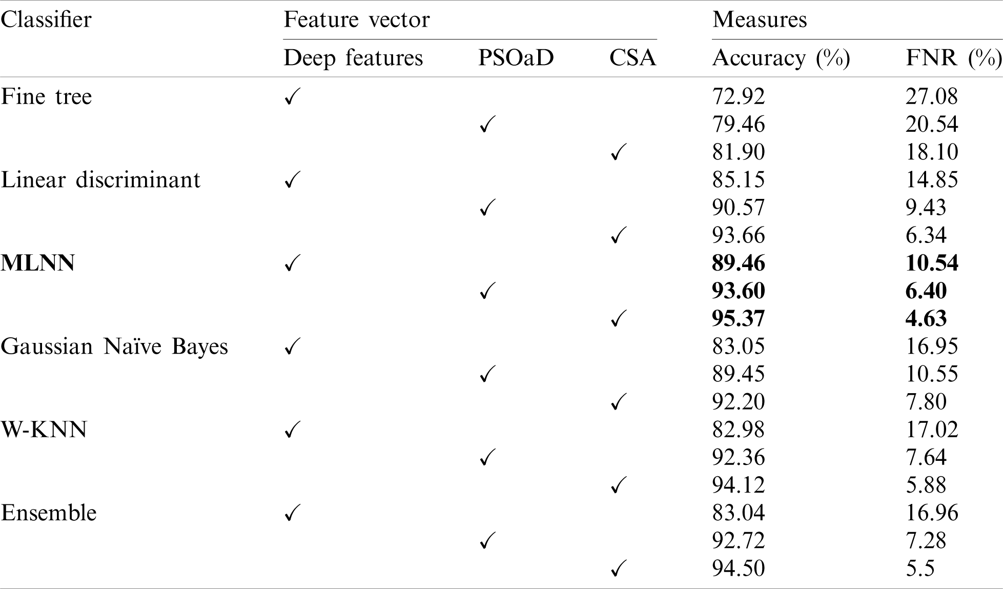
Initially, results are computed on individual feature vectors to analyze the performance of the proposed framework. Tab. 1 describes the classification results of individual feature vectors such as original extracted deep features from GAP layer, GAP features optimization using PSOaD method, and CSA based deep features optimization. Fine trees achieve 72.92% accuracy for original deep features, whereas, on PSOaD and CSA, the achieved accuracy is 79.46% and 81.90%. This accuracy shows that the optimization process improves the accuracy of up to an average 8%. Similarly, the computed accuracy for the linear discriminant classifier is 85.15%, 90.57%, and 93.66% for deep features, PSOaD, and CSA, respectively. The best accuracy is achieved on MLNN of 95.37. The original deep features accuracy of MLNN is 89.46%, whereas 93.60% for PSoaD. Based on the accuracy, we can easily observe that the optimization of features provides better results than original features.
Table 1: Classification accuracy on individual feature vectors on multiple classifiers
4.2 Proposed Fusion Results for 
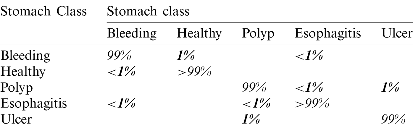
In this experiment, we computed results using the proposed optimal features fusion. We used several optimal features to perform experiments for the evaluation of the proposed technique. This experiment’s main goal is to analyze fusion performance compared to individual algorithms on a selected dataset. Tab. 2 shows this experiment’s result and achieves the best accuracy of 99.3% with a 99% F1 score. The other calculated measures are the precision rate of 98.8%, sensitivity is 99.2%, and FNR is 0.7%. The second-best performance is achieved by 98.6% for W-KNN and Ensemble classifier. However, the lowest achieved accuracy was 84.4% using fine trees. The performance of MLNN is also given in Tab. 3. This table shows each class’s classification accuracy separately, such as bleeding 99%, ulcer 99%, etc. Based on this accuracy, it can prove the performance of the proposed method on the selected dataset. The time noted during the classifier prediction is also given in Tab. 2, which shows the Fine Tree outperforms, but its accuracy is too low compared to MLNN. Hence, overall, MLNN provides better accuracy for this experiment.
Table 2: Classification results using proposed fusion at  on selected dataset
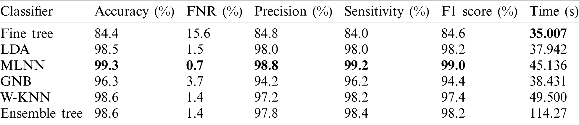
Table 3: Confusion matrix of MLNN for proposed fusion at  on selected dataset
4.3 Proposed Fusion Results Using 
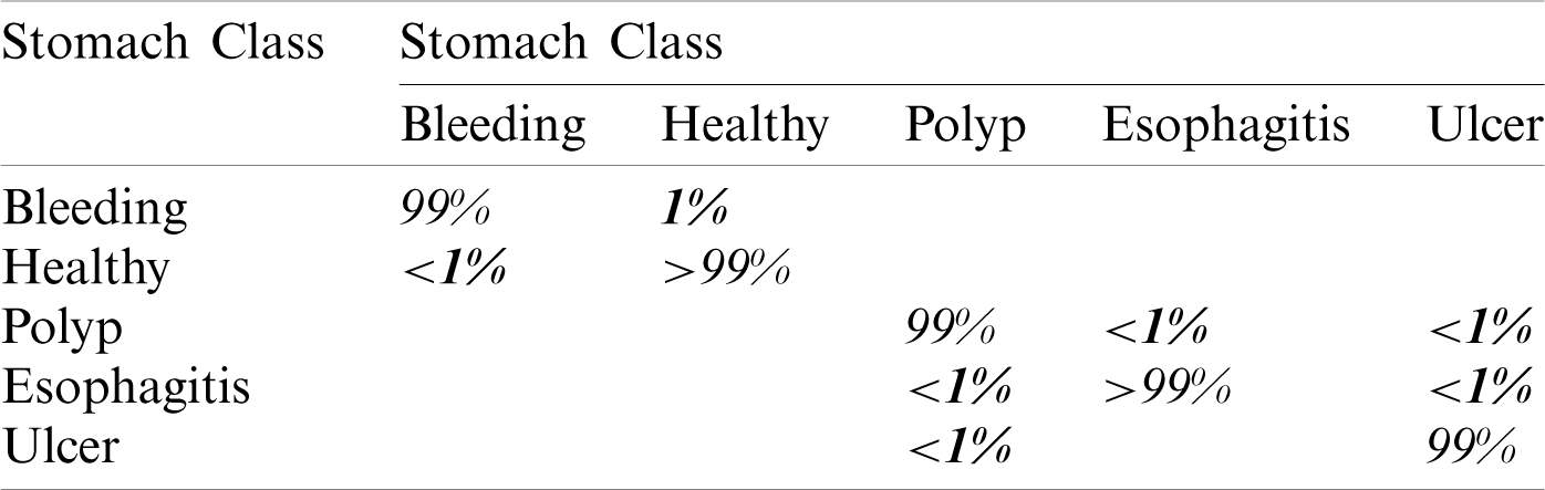
In this experiment, we fused both optimal vectors using the maximal fusion approach and perform classification. It is noted that the fusion process improves accuracy, but time is also increased. The results are given in Tab. 4. This table shows that MLNN better accuracy than other methods like the fine tree, naïve bayes, etc. The accuracy of MLNN is 99.5%, which is improved up to an average 0.4%. The other measures for MLNN are FNR (0.5%), precision rate of 96%, sensitivity of 99.5%, and F1 Score is 97.7%. The prediction time is also noted at 48.83 (s). The linear discriminant classifier also performed well and achieved an accuracy of 99.3%, where the consume time was 42.451 (s). This classifier’s accuracy is also improved compared to results on CV at 15 up to 0.8%. Fine Tree achieves the worst classification accuracy of 85.1%. But the prediction time of this classifier is best as compared to all other methods. Tab. 5 described the proposed method’s authenticity in terms of each class’s correctly predicted accuracy. Based on this table it shows that the proposed method outperforms MLNN.
Table 4: Classification results using proposed fusion at CV=10 on selected dataset
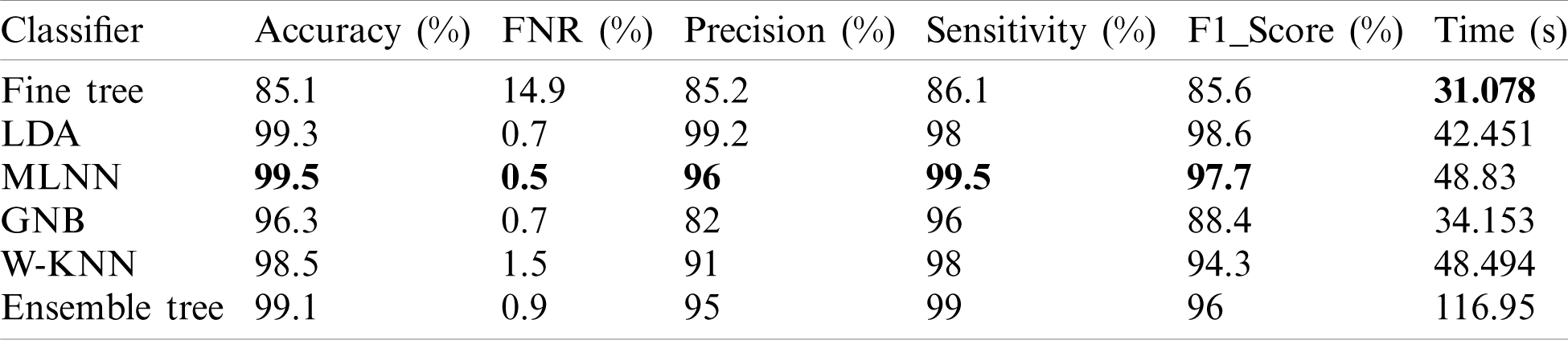
Table 5: Confusion matrix of MLNN using proposed framework at 
4.4 Proposed Fusion Results Using 
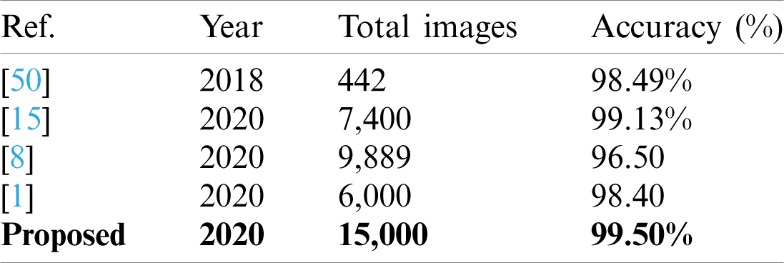
A detailed discussion of proposed classification results is presenting in this section. The main flow is shown in Fig. 1, which shows the proposed method executed in the series of steps, and each step is connected with the previous step. It means the input of each step is directly affected by the system performance. The results are computed in different steps to analyze the strength of each step. Initially, deep features are extracted from enhanced WCE images and retrained Inception V3 CNN model using deep transfer learning. After that, two optimization techniques are implemented and passed deep feature vector at the same time. In the output, two resultant vectors are obtained, and we test both vectors separately, as results are given in Tab. 1. This table, it is showing that the results are improved after applying optimization techniques. An average 8% change is occurred in the results after applying PSOaD and CSA. The maximum achieved accuracy in this table is 95.37%. Later, we fused both optimal vectors using a maximal approach and perform classification using MLNN. After fusion, the results are computed using two cross-validation values—15 and 10. The 15-fold cross-validation results are given in Tab. 2 and confirm through Tab. 3. Tab. 2 shows the maximum results of 99.1% on MLNN, whereas the minimum noted accuracy is 84.4%. Tab. 4 shows the 10-fold validation results and achieved an accuracy of 99.5%, where the minimum attained accuracy is 85.1%. The 99.5% accuracy of MLNN is proved through Tab. 5. In addition, the prediction and training time is also noted. The prediction time is given in Tab. 2 and 4 and shows that the fine tree performs more efficiently than all other classifiers. Still, the accuracy of this classifier is not sufficient.In the choice of pre-trained model, we also compare with other deep neural nets like AlexNet, VGG16, VGG19, GoogleNet, and ResNet50 with Inception V3. We just replace the pre-trained model in Fig. 1 and compute results by employing the same steps. Results are visually plotted in Fig. 6. This figure, it is showing that the selection of Inception V3 is works well. The ResNet50 also gives an accuracy of 97.52%, which is the second highest compared to other techniques. The overall time of MLNN is also plotted in Fig. 7. This figure shows that individual optimization steps consume the lowest time than the proposed method, but the proposed step’s accuracy is much better. Hence, the overall proposed method is performed more efficiently for the classification of selected stomach infections. Tab. 6 shows the comparison of the proposed method with existing techniques. In [50], the authors used 442 WCE images for the experimental process and achieved an accuracy of 98.49%. In [15], 7,400 WCE images are used by authors and attained an accuracy of 99.13%. Later in [8] images are increased and achieved an accuracy of 96.50%. In this work, we were using 15,000 images and achieved an accuracy of 99.50%, which is better than these listed methods.
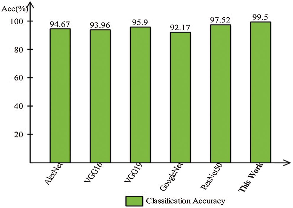
Figure 6: Comparison of this work model selection with other pre-trained models
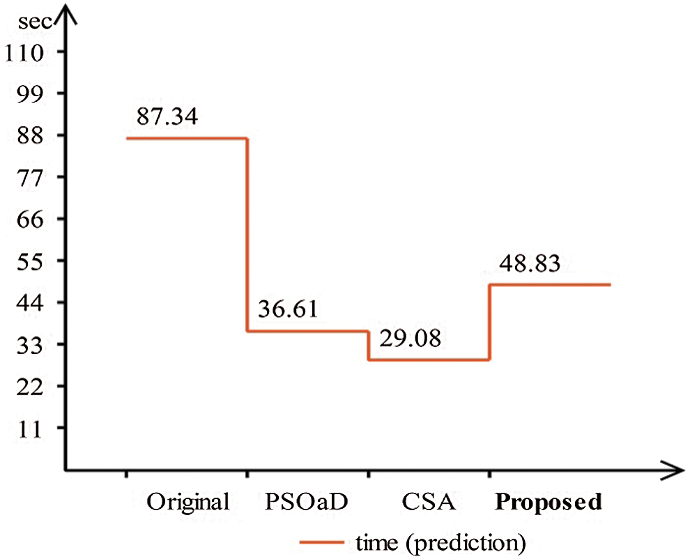
Figure 7: Prediction time comparison of proposed framework with individual steps
Table 6: Comparison with existing techniques
Besides, we also computed the confidence interval of the proposed method. We consider the confidence level 95%,  , and the resultant standard deviation is 0.4,
  is 0.2828, and margin of error is
  (
( 0.56%). This confidence interval shows that the proposed method accuracy is consistent and significantly better for all confidence levels, as shown in Fig. 8.
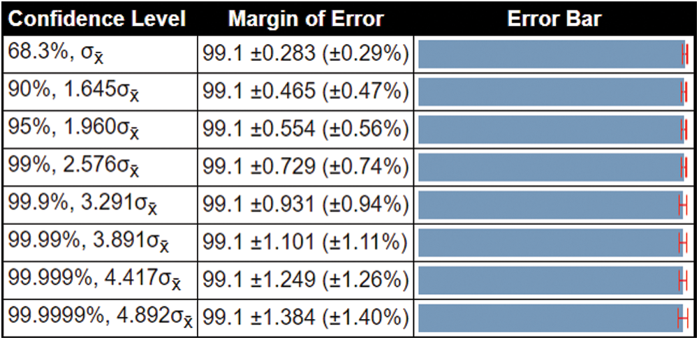
Figure 8: Confidence interval of the proposed method
A deep features optimization-based design is implemented in this article for stomach infections classification using WCE images. In the presented design, deep learning features are computed through TL and optimized using two metaheuristic algorithms- PSOaD and CSA. Both algorithms’ performance is separately evaluated and analyzed, each with original extracted deep learning features. Based on the original features, the optimal vectors better accuracy of 93.60% and 95.37%, whereas the original features highest accuracy was 89.46%. Fused both optimal vectors in the next step and feed in MLNN for final classification. This step gives an accuracy of 99.5%, which is improved compared to individual features and existing techniques. The presented results concluded that optimal features’ fusion provides better accuracy than separate optimal sets. Hence, this work’s major primary strength is the optimal feature selection and later fusion by maximal value. However, the major drawback of the fusion process is consuming higher time. Future work will focus on improving the database and construct a CNN model from scratch. Moreover, deep learning will be elected to consider the problem of ulcer and polyp segmentation.
Funding Statement: This research was supported by Korea Institute for Advancement of Technology (KIAT) grant funded by the Korea Government (MOTIE) (P0012724, The Competency Development Program for Industry Specialist) and the Soonchunhyang University Research Fund.
Conflicts of Interest: The authors declare that they have no conflicts of interest to report regarding the present study.
1. M. A. Khan, S. Kadry, M. Alhaisoni, Y. Nam, Y. Zhang et al. (2020). , “Computer-aided gastrointestinal diseases analysis from wireless capsule endoscopy: A framework of best features selection,” IEEE Access, vol. 9, pp. 132850–132859. [Google Scholar]
2. A. Liaqat, M. A. Khan, M. Sharif, M. Mittal, T. Saba et al. (2020). , “Gastric tract infections detection and classification from wireless capsule endoscopy using computer vision techniques: A review,” Current Medical Imaging, vol. 1, pp. 1–23. [Google Scholar]
3. A. C. Society. (2020). “Cancer facts and figures,” . [Online]. Available: https://seer.cancer.gov/statfacts/html/stomach.html. [Google Scholar]
4. A. C. Society. (2020). “Key statistics about stomach cancer,” . [Online]. Available: https://www.cancer.org/cancer/stomach-cancer/about/key-statistics.html. [Google Scholar]
5. G. Iddan, G. Meron, A. Glukhovsky and P. Swain. (2000). “Wireless capsule endoscopy,” Nature, vol. 405, no. 6785, pp. 417–417. [Google Scholar]
6. M. Pennazio, C. Spada, R. Eliakim, M. Keuchel, A. May. (2015). et al., “Small-bowel capsule endoscopy and device-assisted enteroscopy for diagnosis and treatment of small-bowel disorders: European Society of Gastrointestinal Endoscopy (ESGE) Clinical Guideline,” Endoscopy, vol. 47, no. 4, pp. 352–386. [Google Scholar]
7. D. G. Adler and C. J. Gostout. (2003). “Wireless capsule endoscopy,” Hospital Physician, vol. 39, pp. 14–22. [Google Scholar]
8. A. Majid, M. A. Khan, M. Yasmin, A. Rehman, A. Yousafzai et al. (2020). , “Classification of stomach infections: A paradigm of convolutional neural network along with classical features fusion and selection,” Microscopy Research and Technique, vol. 83, no. 5, pp. 562–576. [Google Scholar]
9. M. A. Mohammed, B. Al-Khateeb, A. N. Rashid, D. A. Ibrahim, M. K. Abd Ghani et al. (2018). , “Neural network and multi-fractal dimension features for breast cancer classification from ultrasound images,” Computers & Electrical Engineering, vol. 70, pp. 871–882. [Google Scholar]
10. M. A. Mohammed, K. H. Abdulkareem, S. A. Mostafa, M. K. A. Ghani, M. S. Maashi et al. (2020). , “Voice pathology detection and classification using convolutional neural network model,” Applied Sciences, vol. 10, pp. 3723. [Google Scholar]
11. M. Subathra, M. A. Mohammed, M. S. Maashi, B. Garcia-Zapirain, N. Sairamya et al. (2020). , “Detection of focal and non-focal electroencephalogram signals using fast walsh-hadamard transform and artificial neural network,” Sensors, vol. 20, pp. 4952. [Google Scholar]
12. M. K. Abd Ghani, M. A. Mohammed, N. Arunkumar, S. A. Mostafa, D. A. Ibrahim et al. (2020). , “Decision-level fusion scheme for nasopharyngeal carcinoma identification using machine learning techniques,” Neural Computing and Applications, vol. 32, no. 3, pp. 625–638. [Google Scholar]
13. D. Shen, G. Wu and H. I. Suk. (2017). “Deep learning in medical image analysis,” Annual Review of Biomedical Engineering, vol. 19, no. 1, pp. 221–248. [Google Scholar]
14. M. A. Khan, M. Rashid, M. Sharif, K. Javed and T. Akram. (2019). “Classification of gastrointestinal diseases of stomach from WCE using improved saliency-based method and discriminant features selection,” Multimedia Tools and Applications, vol. 78, no. 19, pp. 27743–27770. [Google Scholar]
15. H. T. Rauf, U. Shoaib, M. I. Lali, M. Alhaisoni, M. N. Irfan et al. (2020). , “Particle swarm optimization with probability sequence for global optimization,” IEEE Access, vol. 8, pp. 110535–110549. [Google Scholar]
16. M. A. Khan, M. Sharif, T. Akram, M. Yasmin and R. S. Nayak. (2019). “Stomach deformities recognition using rank-based deep features selection,” Journal of Medical Systems, vol. 43, no. 12, pp. 329. [Google Scholar]
17. M. A. Khan, Y. D. Zhang, S. A. Khan, M. Attique, A. Rehman et al. (2020). , “A resource conscious human action recognition framework using 26-layered deep convolutional neural network,” Multimedia Tools and Applications, vol. 10, pp. 1–23. [Google Scholar]
18. A. Krizhevsky, I. Sutskever and G. E. Hinton. (2017). “Imagenet classification with deep convolutional neural networks,” Communications of the ACM, vol. 60, no. 6, pp. 84–90. [Google Scholar]
19. K. Simonyan and A. Zisserman. (2014). “Very deep convolutional networks for large-scale image recognition,” arXiv preprint arXiv: 1409.1556. [Google Scholar]
20. K. He, X. Zhang, S. Ren and J. Sun. (2016). “Deep residual learning for image recognition,” in Proc. of the IEEE Conf. on Computer Vision and Pattern Recognition, Las Vegas, USA, pp. 770–778. [Google Scholar]
21. C. Szegedy, W. Liu, Y. Jia, P. Sermanet, S. Reed et al. (2015). , “Going deeper with convolutions,” in Proc. of the IEEE Conf. on Computer Vision and Pattern Recognition, Boston, Massachusetts, pp. 1–9. [Google Scholar]
22. J. Deng, W. Dong, R. Socher, L. J. Li, K. Li et al. (2009). , “Imagenet: A large-scale hierarchical image database,” in IEEE Conf. on Computer Vision and Pattern Recognition, Miami, FL, USA, pp. 248–255. [Google Scholar]
23. M. A. Khan, T. Akram, M. Sharif, K. Javed, M. Rashid et al. (2020). , “An integrated framework of skin lesion detection and recognition through saliency method and optimal deep neural network features selection,” Neural Computing and Applications, vol. 32, no. 20, pp. 15929–15948. [Google Scholar]
24. M. A. Khan, M. S. Sarfraz, M. Alhaisoni, A. A. Albesher, S. Wang et al. (2020). , “StomachNet: Optimal deep learning features fusion for stomach abnormalities classification,” IEEE Access, vol. 8, pp. 197969– 197981. [Google Scholar]
25. T. Cogan, M. Cogan and L. Tamil. (2019). “MAPGI: Accurate identification of anatomical landmarks and diseased tissue in gastrointestinal tract using deep learning,” Computers in Biology and Medicine, vol. 111, pp. 103351. [Google Scholar]
26. T. Aoki, A. Yamada, Y. Kato, H. Saito, A. Tsuboi et al. (2020). , “Automatic detection of blood content in capsule endoscopy images based on a deep convolutional neural network,” Journal of Gastroenterology and Hepatology, vol. 35, no. 7, pp. 1196–1200. [Google Scholar]
27. N. Ghatwary, X. Ye and M. Zolgharni. (2019). “Esophageal abnormality detection using densenet based faster R-CNN with gabor features,” IEEE Access, vol. 7, pp. 84374–84385. [Google Scholar]
28. M. A. Khan, M. A. Khan, F. Ahmed, M. Mittal, L. M. Goyal et al. (2020). , “Gastrointestinal diseases segmentation and classification based on duo-deep architectures,” Pattern Recognition Letters, vol. 131, pp. 193–204. [Google Scholar]
29. J. H. Lee, Y. J. Kim, Y. W. Kim, S. Park, Y. I. Choi et al. (2019). , “Spotting malignancies from gastric endoscopic images using deep learning,” Surgical Endoscopy, vol. 33, no. 11, pp. 3790–3797. [Google Scholar]
30. R. Shahril, A. Saito, A. Shimizu and S. Baharun. (2020). “Bleeding classification of enhanced wireless capsule endoscopy images using deep convolutional neural network,” Journal of Information Science & Engineering, vol. 36, no. 1, pp. 91–108. [Google Scholar]
31. R. Zhao, R. Zhang, T. Tang, X. Feng, J. Li et al. (2018). , “TriZ-a rotation-tolerant image feature and its application in endoscope-based disease diagnosis,” Computers in Biology and Medicine, vol. 99, pp. 182–190. [Google Scholar]
32. M. Souaidi, A. A. Abdelouahed and M. El Ansari. (2019). “Multi-scale completed local binary patterns for ulcer detection in wireless capsule endoscopy images,” Multimedia Tools and Applications, vol. 78, no. 10, pp. 13091–13108. [Google Scholar]
33. D. K. Iakovidis, S. V. Georgakopoulos, M. Vasilakakis, A. Koulaouzidis and V. P. Plagianakos. (2018). “Detecting and locating gastrointestinal anomalies using deep learning and iterative cluster unification,” IEEE Transactions on Medical Imaging, vol. 37, no. 10, pp. 2196–2210. [Google Scholar]
34. M. Sharif, M. Attique Khan, M. Rashid, M. Yasmin, F. Afza et al. (2019). , “Deep CNN and geometric features-based gastrointestinal tract diseases detection and classification from wireless capsule endoscopy images,” Journal of Experimental & Theoretical Artificial Intelligence, pp. 1–23. [Google Scholar]
35. P. Sivakumar and B. M. Kumar. (2019). “A novel method to detect bleeding frame and region in wireless capsule endoscopy video,” Cluster Computing, vol. 22, no. S5, pp. 12219–12225. [Google Scholar]
36. M. Dorigo, M. Birattari and T. Stutzle. (2006). “Ant colony optimization,” IEEE Computational Intelligence Magazine, vol. 1, no. 4, pp. 28–39. [Google Scholar]
37. C. Szegedy, V. Vanhoucke, S. Ioffe, J. Shlens and Z. Wojna. (2016). “Rethinking the inception architecture for computer vision,” in Proc. of the IEEE Conf. on Computer Vision and Pattern Recognition, Las Vegas, USA, pp. 2818–2826. [Google Scholar]
38. S. J. Pan and Q. Yang. (2010). “A survey on transfer learning,” IEEE Transactions on Knowledge and Data Engineering, vol. 22, no. 10, pp. 1345–1359. [Google Scholar]
39. M. Oquab, L. Bottou, I. Laptev and J. Sivic. (2014). “Learning and transferring mid-level image representations using convolutional neural networks,” in Proc. of the IEEE Conf. on Computer Vision and Pattern Recognition, Columbus, Ohio, USA, pp. 1717–1724. [Google Scholar]
40. A. Askarzadeh. (2016). “A novel metaheuristic method for solving constrained engineering optimization problems: Crow search algorithm,” Computers & Structures, vol. 169, pp. 1–12. [Google Scholar]
41. A. E. Hassanien, R. M. Rizk-Allah and M. Elhoseny. (2018). “A hybrid crow search algorithm based on rough searching scheme for solving engineering optimization problems,” Journal of Ambient Intelligence and Humanized Computing, vol. 119, no. 4, pp. 117. [Google Scholar]
42. J. Kennedy and R. C. Eberhart. (1997). “A discrete binary version of the particle swarm algorithm,” in IEEE Int. Conf. on Systems, Man, and Cybernetics, Computational Cybernetics and Simulation, Orlando, FL, USA, pp. 4104–4108. [Google Scholar]
43. R. C. Eberhart and Y. Shi. (1998). “Comparison between genetic algorithms and particle swarm optimization,” in Int. Conf. on Evolutionary Programming, Berlin, Heidelberg: Springer, pp. 611–616. [Google Scholar]
44. S. Yadav, A. Ekbal and S. Saha. (2018). “Feature selection for entity extraction from multiple biomedical corpora: A PSO-based approach,” Soft Computing, vol. 22, no. 20, pp. 6881–6904. [Google Scholar]
45. J. Kennedy. (1998). “The behavior of particles,” Evolutionary Programming VII. EP Lecture Notes in Computer Science, in V. W. Porto, N. Saravanan, D. Waagen, A. E. Eiben, (eds.vol 1447. Springer, Berlin, Heidelberg. pp. 579–589. [Google Scholar]
46. M. A. Khan, T. Akram, M. Sharif, M. Y. Javed, N. Muhammad et al. (2019). , “An implementation of optimized framework for action classification using multilayers neural network on selected fused features,” Pattern Analysis and Applications, vol. 22, no. 4, pp. 1377–1397. [Google Scholar]
47. K. Pogorelov, K. R. Randel, C. Griwodz, S. L. Eskeland, T. de Lange et al. (2017). , “Kvasir: A multi-class image dataset for computer aided gastrointestinal disease detection,” in Proc. of the 8th ACM on Multimedia Systems Conf., NY, USA, pp. 164–169. [Google Scholar]
48. J. Silva, A. Histace, O. Romain, X. Dray and B. Granado. (2014). “Toward embedded detection of polyps in WCE images for early diagnosis of colorectal cancer,” International Journal of Computer Assisted Radiology and Surgery, vol. 9, no. 2, pp. 283–293. [Google Scholar]
49. J. Bernal, F. J. Sánchez, G. Fernández-Esparrach, D. Gil, C. Rodríguez et al. (2015). , “WM-DOVA maps for accurate polyp highlighting in colonoscopy: Validation vs. saliency maps from physicians,” Computerized Medical Imaging and Graphics, vol. 43, pp. 99–111. [Google Scholar]
50. A. Liaqat, M. A. Khan, J. H. Shah, M. Sharif, M. Yasmin et al. (2018). , “Automated ulcer and bleeding classification from WCE images using multiple features fusion and selection,” Journal of Mechanics in Medicine and Biology, vol. 18, no. 4, pp. 1850038. [Google Scholar]
 | This work is licensed under a Creative Commons Attribution 4.0 International License, which permits unrestricted use, distribution, and reproduction in any medium, provided the original work is properly cited. |