DOI:10.32604/cmc.2021.014353
| Computers, Materials & Continua DOI:10.32604/cmc.2021.014353 | |
| Article |
Enhanced KOCED Routing Protocol with K-means Algorithm
1Department of Plasma Bioscience and Display, KwangWoon University Graduate School, Seoul, 01897, Korea
2Ingenium College of Liberal Arts, KwangWoon University, Seoul, Korea
3Department of Computer Engineering, Catholic University of Pusan, Busan, Korea
*Corresponding Author: Daesung Lee. Email: dslee@cup.ac.kr
Received: 16 September 2020; Accepted: 11 January 2021
Abstract: Replacing or recharging batteries in the sensor nodes of a wireless sensor network (WSN) is a significant challenge. Therefore, efficient power utilization by sensors is a critical requirement, and it is closely related to the life span of the network. Once a sensor node consumes all its energy, it will no longer function properly. Therefore, various protocols have been proposed to minimize the energy consumption of sensors and thus prolong the network operation. Recently, clustering algorithms combined with artificial intelligence have been proposed for this purpose. In particular, various protocols employ the K-means clustering algorithm, which is a machine learning method. The number of clustering configurations required by the K-means clustering algorithm is greater than that required by the hierarchical algorithm. Further, the selection of the cluster heads considers only the residual energy of the nodes without accounting for the transmission distance to the base station. In terms of energy consumption, the residual energy of each node, the transmission distance, the cluster head location, and the central relative position within the cluster should be considered simultaneously. In this paper, we propose the KOCED (K-means with Optimal clustering for WSN considering Centrality, Energy, and Distance) protocol, which considers the residual energy of nodes as well as the distances to the central point of the cluster and the base station. A performance comparison shows that the KOCED protocol outperforms the LEACH protocol by 259% (223 rounds) for first node dead (FND) and 164% (280 rounds) with 80% alive nodes.
Keywords: WSN; routing protocol; K-means; K-optimal; LEACH; KCE; KOCED
The sensor nodes in a wireless sensor network (WSN) are often installed in large numbers, especially in places that are not easily accessible. This makes it is difficult to replace or recharge their batteries. Consequently, efficient utilization of the limited energy of sensor nodes is a critical requirement [1–3]. Accordingly, one of the most important considerations for designing WSNs is to minimize the energy consumption of each node in order to increase the energy efficiency of the network. Once a wireless sensor node consumes all its energy, it will no longer be available, and if more than a specific number of the total nodes (50%–80%) in the network consume all their energy, the network will not function properly [4–8]. Therefore, various protocols have been proposed to minimize the energy consumption of nodes and thus prolong the network operation. A large number of sensor nodes are placed where the users want to obtain information, and the collected information is passed to the base station. Users or applications can communicate queries or receive data, which are collected from the sensor space through base stations.
The sensor nodes of a WSN are usually installed in places that are difficult to access. Therefore, sensor network protocols should have self-configuring functionality whereby the sensor nodes work in cooperation with each other. Sensor nodes that are deployed on surveillance missions in specific areas detect data that are internally converted into high-level information through data processing procedures of the network. Then, the data are sent to remote administrators. In the routing process, the raw or processed data are transmitted to the final destination over a single hop or multiple hops. These hopping mechanisms are among the many issues that need to be addressed so that WSNs can be employed in various applications. A number of routing protocol studies are under way for this purpose [9,10].
The LEACH protocol is a hierarchical clustering algorithm for efficient energy utilization. It uses a T(n) critical expression for cluster head selection. However, this does not always guarantee that an optimal cluster will be formed. In addition, the number of nodes in a cluster is changeable, i.e., it may be small or large. As the rounds progress, the first node dies. However, if a node with low residual energy is selected as the cluster head (CH), the data transmission is more likely to fail. To prevent nodes with low residual energy from being selected as CHs, this study considers the CH selection probability critical expression.
Wireless sensor protocols that use K-means clustering do not configure clusters after selecting the CHs. The main advantage of this approach is that clusters are uniformly constructed and most of the member nodes of a cluster are evenly distributed in their affiliated clusters. After the clusters are configured, this method selects nodes with high residual energy or nodes that are close to the central point of the cluster as CHs. However, a disadvantage of this approach is that it takes a longer time to form clusters than the LEACH algorithm because the clustering configuration process repeatedly selects the central point to appoint the CHs. Protocols based on K-means clustering consider the residual energy of nodes and the central point to select CHs. Distances for data transmission that involves high energy consumption, especially from CH to BS, are not considered [11–15].
Consequently, using the K-means clustering algorithm in the WSN protocol ensures that the member nodes in the cluster are uniformly distributed. However, it takes a longer time to configure the clusters compared to traditional hierarchical algorithms. In addition, there is a problem of selecting consecutive CHs on the same node because the CH selection considers only the residual energy of the node closest to the central point of the cluster. This drawback consequently reduces the life span of the entire network. Moreover, the overall energy efficiency of the network cannot be considered because the distance to the base station is not taken into account when selecting the CH. Further, the number of clusters (k) is not optimized.
This paper proposes KOCED (K-means with Optimal clustering for WSN considering Centrality, Energy, and Distance), a routing protocol that improves the energy efficiency of the entire network while addressing the above-mentioned problems. A performance comparison shows that the KOCED protocol outperforms the LEACH protocol by 259% (223 rounds) for first node dead (FND) and 164% (280 rounds) with 80% alive nodes.
The remainder of this paper is organized as follows. Section 2 reviews related algorithms. Section 3 presents the KOCED protocol. Section 4 describes the simulations conducted in this study. Finally, Section 5 concludes the paper.
The LEACH (Low-Energy Adaptive Clustering Hierarchy) protocol is a representative clustering-based protocol proposed by Wendy B. Heinzelman [16–20]. It consists of a set-up phase and a steady-state phase. During the set-up phase, the CHs are randomly selected on the basis of a probability threshold and the cluster configuration is performed. For nodes, the probability critical expression used to select the CH, which takes a value between 0 and 1, is given by
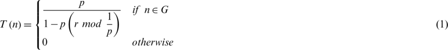
where G is a collection of nodes that have not been selected as CHs until the current round and the previous round. Each node generates a random value between 0 and 1 and compares it to Eq. (1); then, a node that has a lower value than the critical expression is selected as the CH.
The process of forming a cluster is summarized as follows. After the CHs are first selected on the basis of Eq. (1), the CHs broadcast advertising messages containing their own data to the surrounding nodes in the sensor space. The regular nodes that receive the advertising messages from the CHs form the cluster by sending a Join-Request message to the CH with the largest signal strength, i.e., RSSI (received signal strength index). When the cluster configuration is complete, the CH creates a time-division multiple access (TDMA) schedule that tells member nodes when each node will transfer, depending on the number of member nodes. During the steady-state phase, the member nodes in the cluster transmit data to match the TDMA schedule assigned by the CH during the set-up phase. In the steady-state phase, the member nodes transmit data to the CH at their respective operating time (wake), i.e., time to transfer, and return to the sleep state. After all the member nodes send data to the CH, the CH merges the received data and sends it to the base station in a code-division multiple access (CDMA) manner, completing the steady-state phase. The cycle from the set-up stage to the steady-state stage is called a round.
Fig. 1 shows the flowchart for one round of the LEACH protocol. The left part of the flowchart shows the CH selection and the right part shows the cluster configuration. The dashed lines in the flowchart indicate that the CH is in a state of wireless communication. The member nodes receive a cluster association message from the selected CH. The CH sends cluster joining messages to multiple member nodes, and after the cluster is formed, the CH transfers the TDMA schedule to each cluster member node.
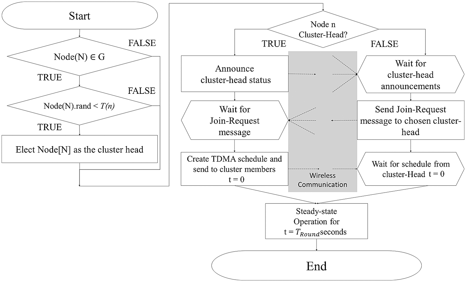
Figure 1: Flowchart of LEACH protocol
K-means clustering [21–28] is a representative clustering algorithm that is based on simple principles but achieves good performance. In K-means clustering, each cluster has one center. Each node belongs to the nearest center, and the nodes assigned to the same center together to form a cluster. K-means clustering should determine the number of clusters in advance. In general, a larger k means more clusters, while a smaller k means fewer clusters. Therefore, the decision of K is crucial. It is typically based on the designer’s heuristics. When the number of sensor nodes is n and they are evenly distributed in a sensor field area of  , the required number of clusters k is calculated as

Another method is to monitor the results by increasing the number of clusters sequentially using the elbow method, as adding another cluster does not improve the modeling of the data significantly. If adding clusters does not produce better results, the number of clusters is set to an optimal value k. Once the K-means clustering has determined the number of clusters k, the initial cluster centroid should be established. This is called the initialization technique, and K-means clustering usually employs the Forgy algorithm for this purpose. The Forgy algorithm tends to spread the center of gravity of each cluster from its center, because the initial cluster is set by any k point(s). Because of these characteristics, the Forgy algorithm is preferred. The EM algorithm consists of the expectation step and the maximization step, and K-means clustering operates repeatedly until the EM algorithm converges. K-means clustering employs EM algorithms because the location of each cluster center point and the cluster to which each node belongs must be found at the same time.
—Step 1: Randomly extract the locations of k nodes from the sensor space and set this node location as the center point of each cluster (set initial value).
—Step 2: Each node in the sensor space obtains the distance from each of the k cluster center points and calculates which one is the closest. The cluster is then constructed using the closest center point (configure clusters).
—Step 3: Move the center point of the cluster by calculating the location average of the nodes in the cluster, i.e., the average of the node locations in the cluster configured in Step 2 is calculated and the center point is changed.
—Step 4: Repeat Steps 2 and 3 until the center point position does not change.
Fig. 2 shows the flowchart of the K-means clustering algorithm.
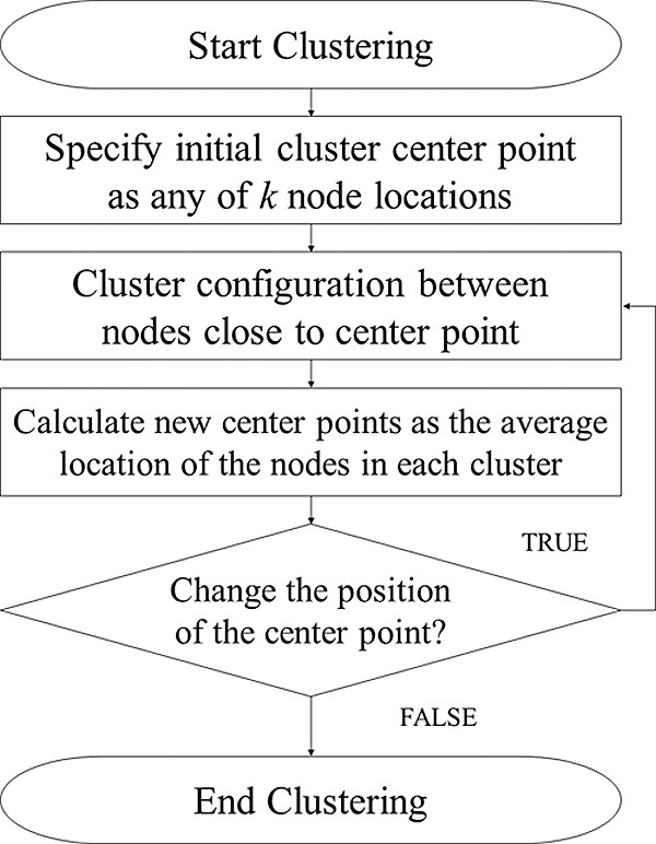
Figure 2: Flowchart of K-means clustering
The K-means clustering algorithm can obtain an objective function J, which is the sum of the distances between the nodes of the cluster and the center point of the cluster when a cluster is established. The smaller the sum, the lower is the value that can be obtained. The objective function J is given by

In Eq. (3), Z is the cluster center point and A is the  matrix representing the allocation information of the node. If the i-th node is assigned to the j-th cluster, aij is 1; otherwise, it is 0. Further, dist(x, z) is a function that measures the distance between x and z. As the K-means clustering algorithm depends on the initial value of the central point, there is a multi-start K-means algorithm that differentiates the central initial value and performs clustering several times to find the best objective function J. The computational complexity of K-means clustering is O(n), because it does not involve much computing compared to hierarchical clustering. The number of clusters and the number of sensor nodes in a cluster are related to the power consumption. The clustering algorithm has many sensor nodes within a cluster when the number of clusters is small; hence, each sensor node consumes a large amount of energy to send data to the base station. When the number of clusters exceeds a certain threshold, the energy efficiency is reduced owing to collisions and interference between the sensor nodes. K-means clustering has the advantage of uniform cluster configuration compared to the LEACH protocol. However, the cluster configuration takes a longer time and relies on empirical methods to determine the number of clusters k.
The KCE (K-means Centrality with Energy) protocol [28] considers the residual energy of the nodes for CH selection. Because the residual energy is taken into account, nodes with low residual energy are initially not selected as CHs. Because the KCE protocol considers not only the central point and distance of the cluster but also the residual energy of the node when selecting the CH, no single node is selected consecutively until all the residual energy of the node is consumed. Therefore, it does not store how many times each node has been selected as a CH. The KCE protocol does not necessarily select nodes with high residual energy as CHs. The node closest to the center point and having the highest residual energy is selected as the CH. As a selected CH usually consumes more energy for long-distance transmission and internal signal processing, it will not be selected as the CH in the next round because it has less energy than other nodes. Therefore, a node is not selected as the CH until all the residual energy is consumed.
The advantages of the KCE protocol are that the cluster size is uniform and the nodes close to the cluster center point can be selected as CHs to increase the energy efficiency within the cluster. The disadvantage is that the optimization of the number of clusters is empirically achieved when the CHs are selected. This is because it does not take into account the transmission distance to the base station, which involves high energy consumption. Therefore, this paper proposes the KOCED protocol to overcome the above-mentioned problems.
Fig. 3 shows the flowchart of the KCE protocol for cluster head selection.
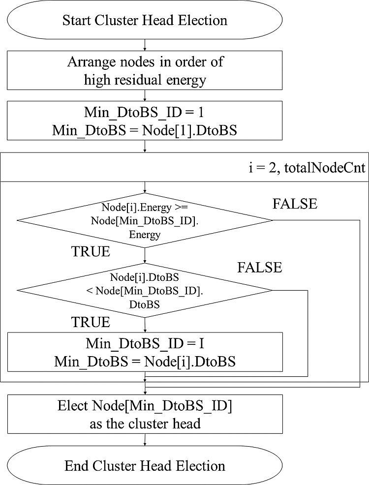
Figure 3: Flowchart of KCE protocol for cluster head selection
The use of the K-means clustering algorithm in the WSN protocol makes the member nodes in each cluster as uniform as possible; however, cluster configuration takes a longer time compared to conventional hierarchical algorithms. In addition, CH selection involves the problem of successive CH selection on the same node by considering only the residual energy of the node or nodes that are close to the center point of the cluster. This reduces the life span of the entire network. Further, when the CH is selected, the distance to the base station is not considered and the number of clusters (k) is not optimized.
This paper proposes KOCED, a protocol that improves the energy efficiency of the entire network while addressing the above-mentioned problems. It involves alternative clustering for WSNs by considering the energy and distance.
• First, to compensate for the shortcoming of long clustering time, the KOCED protocol limits the initial starting conditions and FND of the system. Thus, the clustering process is not performed in each round.
• Second, we want to troubleshoot optimization of the number of clusters (k). Typically, k is set to the number of clusters or close to the number of sensor nodes in the K-means clustering algorithm. However, this study defines and finds the optimal number of clusters (k_opt).
• Third, when selecting a CH, we consider the distance from the center point of the cluster and the residual energy of the node at the same time to overcome the problem of not considering transmission distances to the base station that involve high energy consumption. To solve these problems, the CH is selected by taking into account the residual energy of the node and the distance to the cluster center point or base station.
3.1 Setting When to Configure Clustering
To compensate for the shortcoming of long clustering time, the KOCED protocol is limited to the initial start of the system and the death of the node. This can compensate for the disadvantage of longer time by not performing the clustering process in each round. The procedures for K-means clustering are as follows.
Step 1: The initial center point is designated as an arbitrary sensor node location by the optimal number of clusters (k_opt). Fig. 4 shows the center point of the initial cluster when 10 clusters are employed for 100 sensor nodes in the 100 m  100 m sensor space.
Step 2: Each sensor node is assigned to the nearest cluster center point. Each sensor node is assigned such that the sum ( ) of the squared distance error between the sensor nodes and the center point of the cluster is minimum. The left part of Fig. 5 shows the result of primary clustering obtained through Step 2.
Step 3: The center of the cluster is updated by calculating the average of the sensor nodes within each cluster. This process is shown on the right side of Fig. 5. It can be seen that 10 center points are moved.
The K-means clustering algorithm requires considerable computation and time to construct a cluster compared to the LEACH protocol. To address these problems, it is assumed that no new clusters are to be configured for each round. In other words, the clustering conditions are as follows:
—Perform clustering for the initial round of the sensor space
—Perform clustering only if additional dead nodes occur
Thus, clustering is not performed in each round, which can result in fewer calculations and time savings by the K-means clustering algorithm.
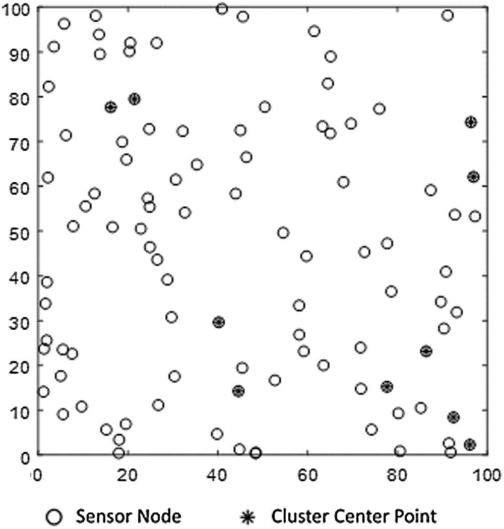
Figure 4: First cluster setting of central point
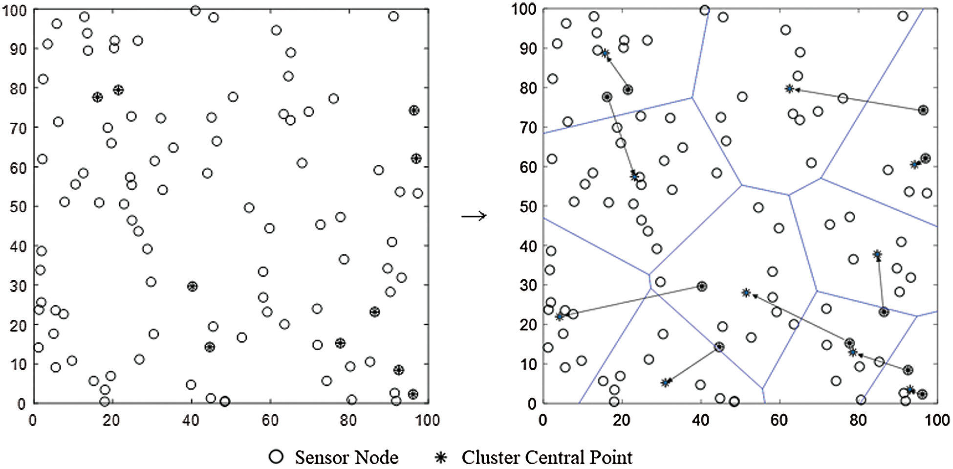
Figure 5: Comparison of initial and final central points of each cluster
3.2 Estimate the Optimal Number of Clusters
To solve the problem of optimizing the number of clusters (k), usually, the K-means clustering algorithm sets k to the number of clusters or close to the number of sensor nodes. However, to define and induce the optimal number of clusters, kopt, the cluster-based WSN protocol uses the multi-hop transfer method via the CH, which reduces the network energy consumption and improves the network life span. As the network life span depends on the number of CHs, i.e., the number of clusters (k), it is important to define the optimal number of clusters (kopt) to maximize the network life span. In particular, the K-means clustering algorithm fails to maximize the network life span by arbitrarily defining the number of clusters or determining the number of nodes to be n, which is an empirical value of  or close to it. Therefore, we try to solve these problems by optimizing the clustering numbers using an energy model expression. For this purpose, the total energy consumed per round is calculated and the energy consumed per round is minimized. This allows us to define the optimal number of clusters.
In an  sensor field, assuming that the k clusters are evenly sized, the area of each cluster is
  . If the radius of a cluster with one CH is R, then the cluster area is
  . One CH is in the radius,
  , of the cluster. It is assumed that all the nodes are evenly distributed in the sensor field, where the number of nodes per cluster field is given by
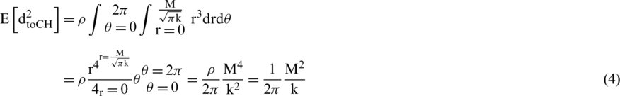
  . Eq. (4) shows the expected value of the square of the distance from the node to the CH,
  .
.
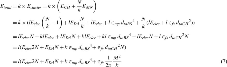
The total energy ( ) consumed per round is then equal to the consumed energy (
 ) of each cluster multiplied by the number of CHs (k). Therefore, the energy consumption of a cluster (
 ) is equal to the sum of the energy consumed by the CH (ECH) and the energy consumed (EMN) by the member nodes in that cluster, with ECH and EMN given by


where l represents the bit size of the packet, Eelec represents the amount of energy used to send and receive data, dtoBS denotes the distance to the base station, dtoCH denotes the distance to the CH,  represents the amount of energy needed for amplification,
  represents the amount of energy needed for amplification in free space, and
  represents the amount of energy needed for amplification in multi-path propagation.
Assume that each cluster has the same number of nodes and the number of member nodes per cluster is  . However, for convenience of calculation, the energy consumption is approximated to
  and calculated as follows:
If the total energy  ) consumed per round is left differential for k and 0, the optimal number of clusters can be obtained as follows:
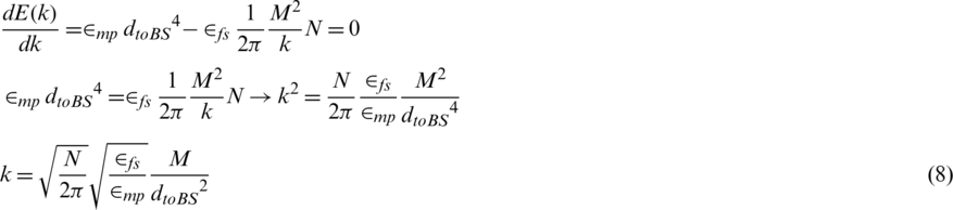
In Eq. (8), if the sensor space is limited to free space, we have 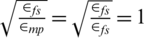 , and the optimum number of clusters can be obtained by obtaining expectations for the distance to the base station. Eq. (9) is an equation for obtaining the expected distance between the node and the sink.
Substituting Eq. (9) into Eq. (8) yields

3.3 Reconfigure Cluster Conditions and How to Select Cluster Head
When selecting CH, we solve the problem of not considering transmissions to the base station by simultaneously considering the distance from the cluster center point or base station and the residual energy of the node.
In general, when considering only the residual energy of nodes in the cluster, the node with the highest residual energy is simply selected as the candidate for the CH. However, considering the residual energy and the distance to the base station, selecting a CH by simple ranking causes energy efficiency issues.
For example, for two nodes A and B, assume that the residual energy in node A is slightly greater than that in node B and the distance to the base station of node A is greater than that of node B. In this case, owing to the high energy consumption over the distance to the base station, node A is selected as the CH. Considering only the residual energy, energy is consumed rapidly and the network life span is reduced.
By modifying the residual energy and distance ranking, the residual energy and distance Score operation for nodes within the cluster is proposed. The CH is selected by giving higher scoring operations on the member nodes that have higher residual energy than the average residual energy for all the nodes in the cluster, i.e., satisfying  . The advantage of this approach is that it reduces the amount of computation in the selection.


The Score is divided into  based on the base station distance and
  based on the cluster center point, defined as Eqs. (11) and (12), respectively.
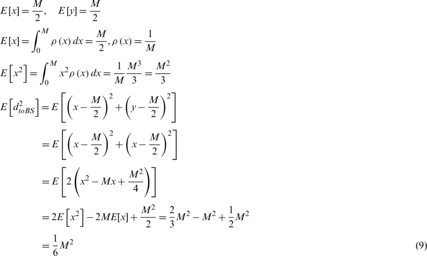
  denotes the current residual energy of the node, Einit denotes the initial energy of the node, dtoBS denotes the distance between the node and the base station, and dtoCC denotes the distance between the node and the center of the cluster. The ratio of the residual energy to the initial energy, the first term in Eqs. (11) and (12), denotes the relative size (normalization value) of the residual energy. It takes a value between 0 to 1 and decreases to 0 as the rounds progress. In addition, the second term of Eqs. (11) and (12) has a value greater than or less than 1 or equal to 0 as the normalized term for distance. The greater the first term and the smaller the second term, the higher is the probability of being selected as the CH. In other words, if the Score values in Eqs. (11) and (12) are large, they are selected as CHs. In the proposed scheme, a node with high residual energy or a node close to the cluster center can be determined using the score calculation for all the nodes in the cluster. Tab. 1 can be referred to when calculating the score for the node information in the cluster. For a total of 10 nodes, the residual energy and distance information of base stations were expressed as normalized values.
Table 1: Information about nodes in the cluster
The results from Tab. 1 show that the node with MAX ( ) is node number 7. Thus, by applying the proposed Score operation, a more appropriate CH can be selected compared to the ranking method by alignment.
For the member nodes satisfying  within each cluster, the operations of
  and
and  of Eqs. (11) and (12) were performed, respectively. In addition, nodes with values MAX (
 ) and MAX (
 ) were selected as CH candidates.
If a node in the cluster has a maximum Score value for the distance to both the base station and the cluster center point, it is selected as the CH. However, if a node with a value of MAX ( ) and a node with a value of MAX (
 ) are different, the CH is determined by calculation.
To predict the energy consumption of two CH candidate nodes, the sum of the distance from the member nodes in the cluster and the distance from the base station, i.e. the total transmission distance, is calculated.  , i.e., the total transmission distance for node i, can be obtained as follows:

where the first term is the distance ( ) from the i-th node to the base station, and the second term is the sum of the distances between the i-th node and the other nodes in the cluster. After the calculations, a sensor node having a shorter total transmission distance is finally selected as the CH. If multiple nodes with the same score are selected as CH candidates, the node closest to the base station of
  and the node closest to the cluster center point of
  are selected as CH candidates. In addition, if the values of MAX (
 ) and MAX (
 ) are the same for the CH candidates, the shorter the distance to the base station, the lower is the energy consumption; hence, the node with MAX (
 ) is selected as the CH.
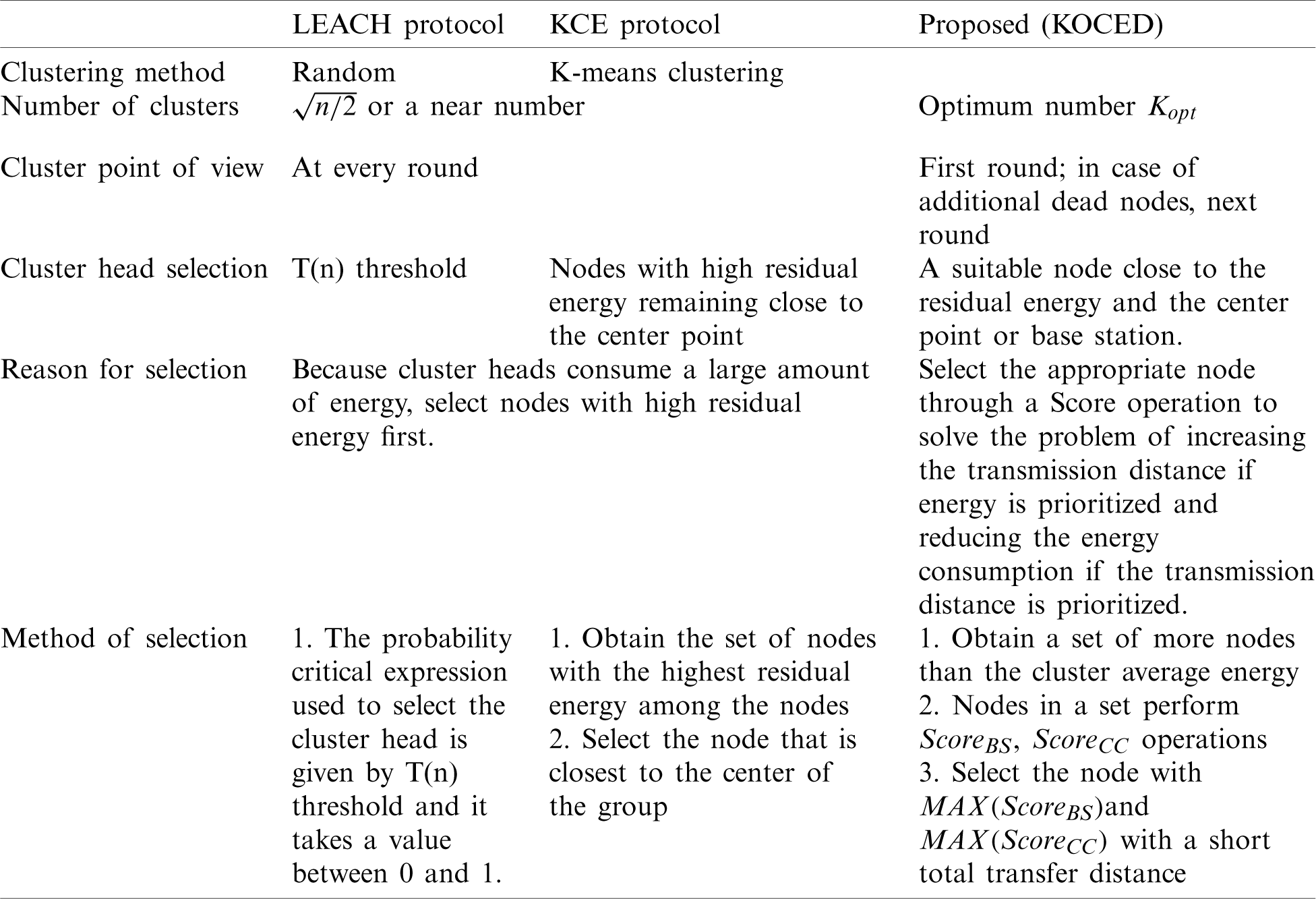
3.4 Comparison of LEACH, KCE, and KOCED
The LEACH, KCE, and KOCED approaches are compared in Tab. 2.
Table 2: Comparison of LEACH, KCE, and KOCED
To verify the energy efficiency of the proposed routing protocol, we compared it with the LEACH protocol and the KCE protocol using the MATLAB simulator.
The parameters for the performance simulation were set as follows. We assumed that after 100 sensor nodes are randomly created in a simulated environment, all the nodes are fixed and have the same initial energy value. Further, the base station is located outside the sensor field. The specific simulation parameters are defined in Tab. 3. The size of the sensor field is  , the location of the base station is (50, 150)/(100, 300)/(200, 600), the initial energy of the sensor node is 0.5 J, EDA is the data aggregating energy dissipation, Eelec is the transmission energy consumption, and
  denote the amplification energy dissipation per volume.
Table 3: Simulation energy model
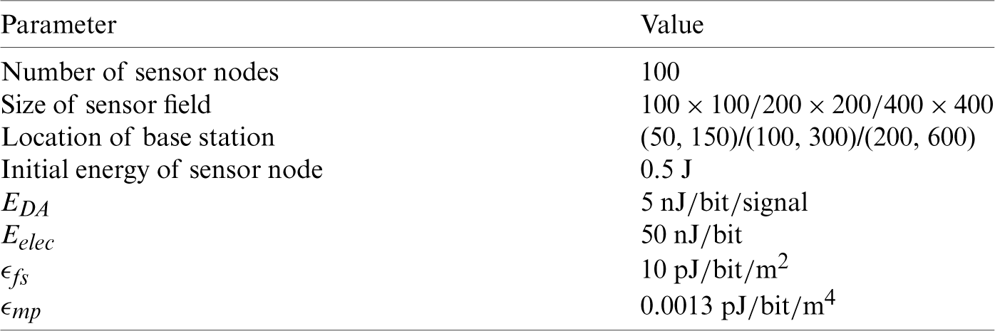
Fig. 6 shows the centrality of the clustering configuration in the LEACH, KCE, and KOCED routing protocols. The KCE and KOCED protocols configure clustering until it converges into the elbow method of the K-means algorithm. At this time, the objective function J is derived to obtain the resulting value, which is the sum of the distances between the nodes of the cluster and the center point of the cluster. Fig. 6 shows that the KCE and KOCED protocols have centrality within the cluster.
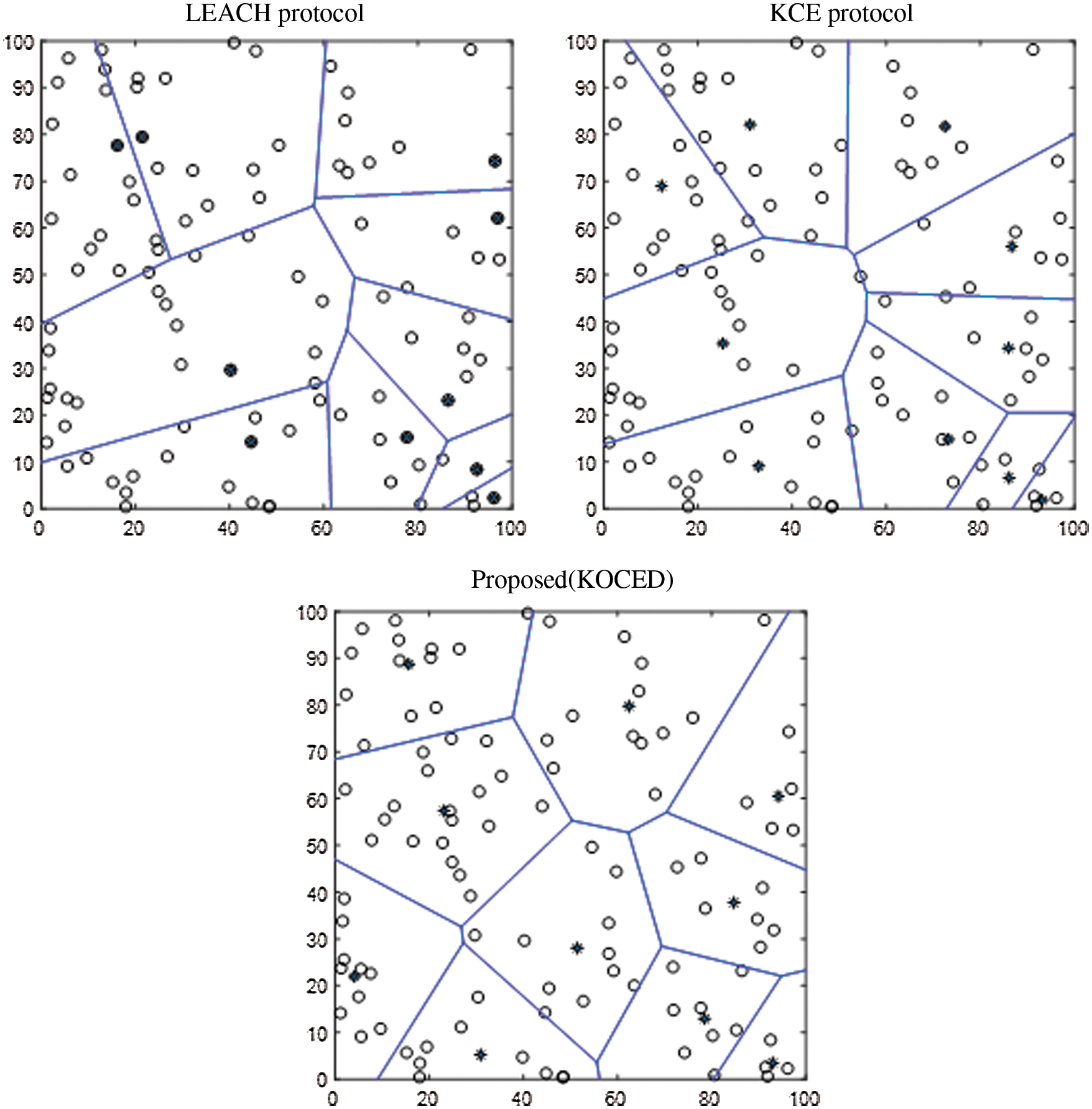
Figure 6: Centrality for configuring clustering for each protocol (a) LEACH protocol (b) KCE protocol (c) Proposed(KOCED)
The following are the results of timing adjustments to overcome the shortcoming of the clustering configuration time. The average clustering configuration time per round for the KCE protocol is around 22 s and that for the KOCED protocol is around 7 s. The total sum of the clustering configuration times is approximately 210 min for the KCE protocol and 75 min for the KOCED protocol. Tab. 4 and Fig. 7. show the time required for the clustering configuration in each round of the KCE protocol and the KOCED protocol. The KCED protocol takes a longer time for cluster formation, whereas the KOCED protocol needs a shorter time.
Table 4: Simulation result: network life span
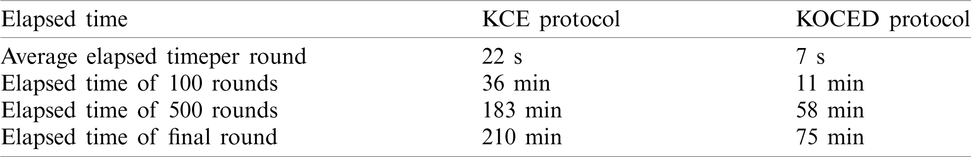
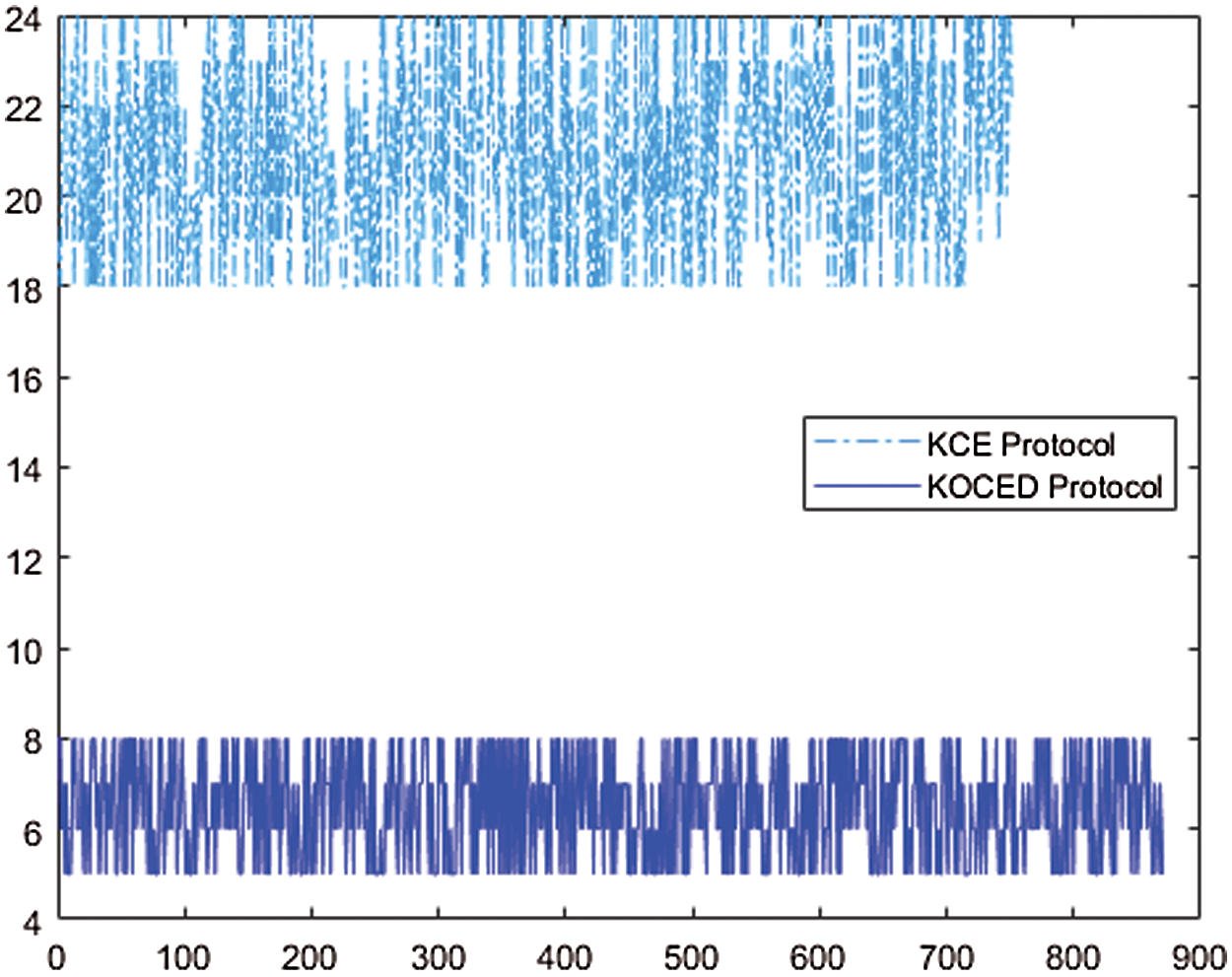
Figure 7: Simulation result: graph showing alive nodes by round
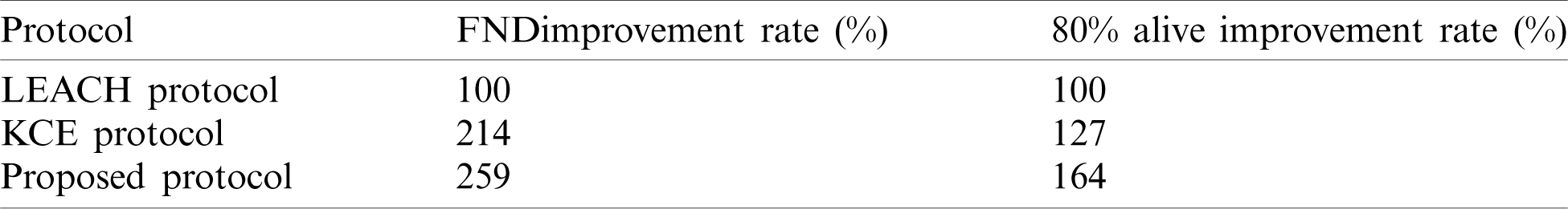
The simulation environment is  depending on the size of the sensor field, as shown in Fig. 8. The base station is located at (50, 150)/(200, 400)/(400, 600). The proposed protocol outperforms the LEACH protocol by 259% in terms of FND. It can be seen that there is a 21% improvement in terms of FND compared to the KCE protocol. FND appeared in the LEACH protocol. Then, it occurred in the KCE protocol. Finally, it occurred in the KOCED protocol. In terms of the occurrence of 80% alive nodes, all the protocols are the same. In particular, the simulation results showed that KOCED has the longest rounds with a uniform routing protocol at 50% alive nodes. Tabs. 5 and 6 compare the three protocols in terms of the network life span. In LEACH, KCE, and KOCED, FND occurred in round 86, 184, and 223, respectively, and 80% alive nodes occurred in round 171, 217, and 280, respectively. In addition, Tab. 6 shows that the rounds for the occurrence of FND and 80% alive nodes increased by 214% and 127% for the KCE protocol, and by 259% and 164% for KOCED.
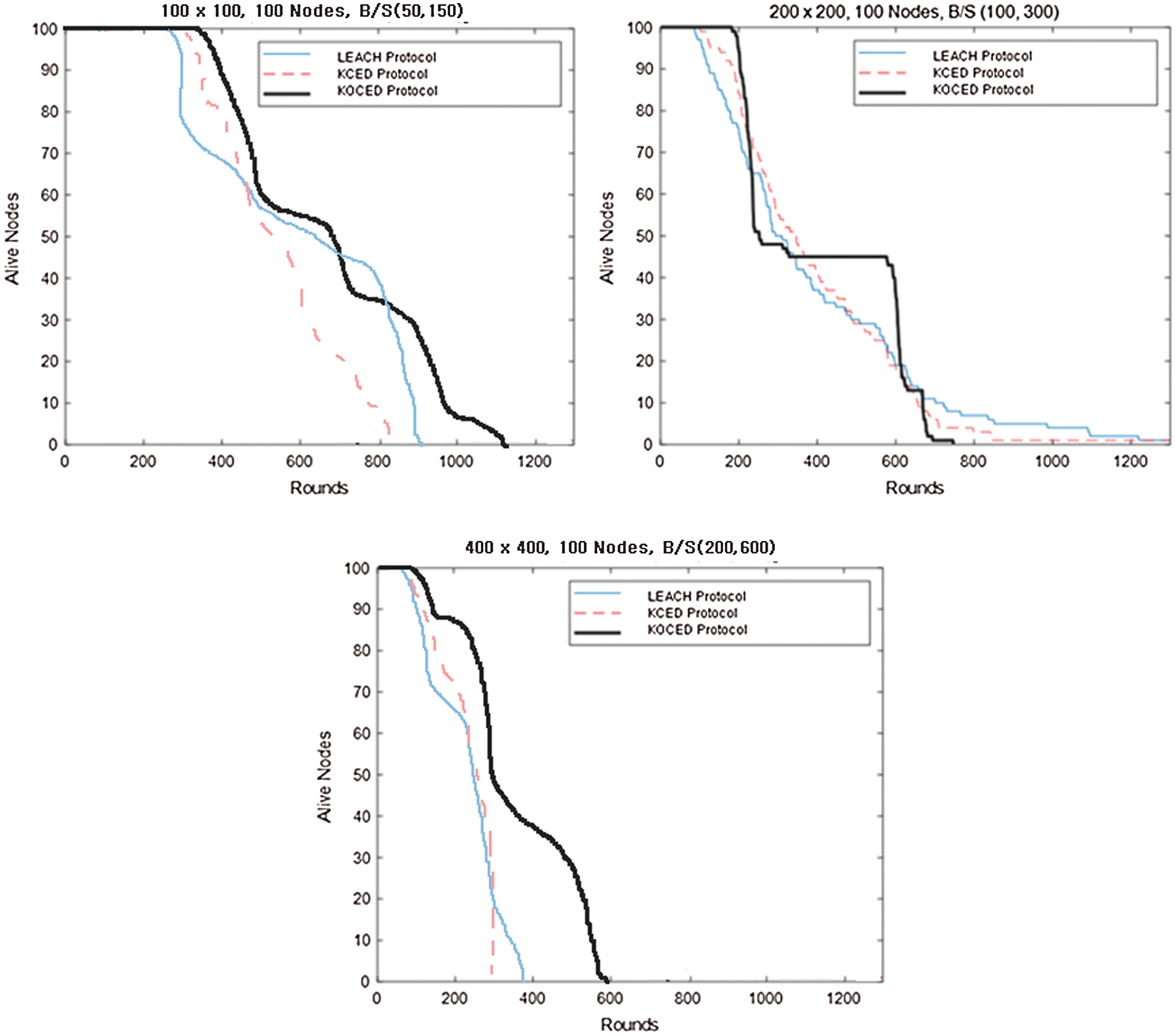
Figure 8: Simulation result: graphs showing alive nodes by round
Table 5: Simulation result: network life span
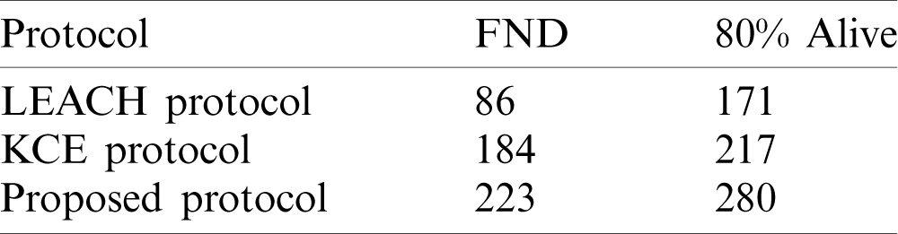
Table 6: Simulation result: network life span improvement rate
The LEACH protocol considers a probability critical expression for cluster selection and formation. Its disadvantages are that it does not provide the density information for each node and it does not optimize the number of cluster heads in a specific network. The disadvantages of the K-means clustering algorithm are that it requires a long clustering formation time and it does not consider the transmission distances from the sensors to the base stations. To overcome these drawbacks, this paper proposed, KOCED, a routing protocol that improves the energy efficiency of the entire network by simultaneously considering the centrality, residual energy, and transmission distances. KOCED achieves efficiency improvement in three steps. First, by reducing the clustering configuration time, it starts cluster formation only when a sensor node is dead in the initial round. This can compensate for unnecessary clustering. Second, it determines the optimal value in a randomly distributed sensor field. This value in normal K-means clustering algorithms is set as the same number of clusters or cluster heads. However, we define the optimal number of clusters, k_opt, on the basis of Eq. (10). Third, KOCED considers the residual energy of the nodes as well as distances to the central position of the cluster and the base station. Thus, KOCED shows excellent performance in terms of energy efficiency. A performance comparison showed that the KOCED protocol outperforms the LEACH protocol by 259% (223 rounds) for FND and 164% (280 rounds) with 80% alive nodes. In the future, we will check the performance reliability of KOCED for cluster optimization and energy consumption with heterogeneous sensor data.
Funding Statement: The authors received no specific funding for this study.
Conflicts of Interest: The authors declare that they have no conflicts of interest to report regarding the present study.
1. Callaway Jr. and H. Edgar. (2003). Wireless Sensor Networks: Architectures and Protocols. Boca Raton, Florida, United States: CRC Press. [Google Scholar]
2. I. F. Akyildiz, W. Su, Y. Sankarasubramaniam and E. Cayirci. (2002). “Wireless sensor networks: A survey,” Computer Networks, vol. 38, no. 4, pp. 393–422. [Google Scholar]
3. C. S. Raghavendra, K. M. Sivalingam and T. Znati. (2006). “Wireless sensor networks,” in Self. Bostonelf: Kluwer Academic Publishers. [Google Scholar]
4. A. Mainwaring, D. Culler, J. Polastre, R. Szewczyk, J. Anderson et al. (2002). , “Wireless sensor networks for habitat monitoring,” in Proc. of The 1st ACM Int. Workshop on Wireless Sensor Networks and Applications, Atlanta, Georgia, USA, pp. 88–97. [Google Scholar]
5. A. Perrig, J. Stankovic and D. Wagner. (2004). “Security in wireless sensor networks,” Communications of the ACM, vol. 47, no. 6, pp. 53–57. [Google Scholar]
6. W. Ye, J. Heidemann and D. Estrin. (2002). “An energy-efficient MAC protocol for wireless sensor networks,” in Twenty-First Annual Joint Conf. of the IEEE Computer and Communications Societies, NY, USA, IEEE, pp. 1567–1576. [Google Scholar]
7. M. Aslam, N. Javaid, A. Rahim, U. Nazir, A. Bibi et al. (2012). , “Survey of extended LEACH-based clustering routing protocols for wireless sensor networks,” in IEEE 14th Int. Conf. on High Performance Computing and Communication & 2012 IEEE 9th Int. Conf. on Embedded Software and Systems, Liverpool, UK, IEEE, pp. 1232–1238. [Google Scholar]
8. A. Braman and G. R. Umapathi. (2014). “A comparative study on advances in LEACH routing protocol for wireless sensor networks: A survey,” International Journal of Advanced Research in Computer and Communication Engineering, vol. 3, no. 2, pp. 5683–5690. [Google Scholar]
9. H. Dhawan and S. Waraich. (2014). “A comparative study on LEACH routing protocol and its variants in wireless sensor networks: A survey,” International Journal of Computer Applications, vol. 95, no. 8, pp. 21–27. [Google Scholar]
10. A. Razaque, M. Abdulgader, C. Joshi, F. Amsaad, M. Chauhan et al. (2016). , “P-LEACH: Energy efficient routing protocol for wireless sensor networks,” in Applications and Technology Conf., Farmingdale, NY, USA, IEEE, pp. 1–5. [Google Scholar]
11. L. Tang and S. Liu. (2011). “Improvement on leach routing algorithm for wireless sensor networks,” in Int. Conf. on Internet Computing and Information Services, Hong Kong, China, IEEE, pp. 199–202. [Google Scholar]
12. M. O. Farooq, A. B. Dogar and G. A. Shah. (2010). “MR-LEACH: Multi-hop routing with low energy adaptive clustering hierarchy,” in Fourth Int. Conf. on Sensor Technologies and Applications, Venice, Italy, IEEE, pp. 262–268. [Google Scholar]
13. F. Xiangning and S. Yulin. (2007). “Improvement on LEACH protocol of wireless sensor network,” in Int. Conf. on Sensor Technologies and Applications (SENSORCOMM 2007Valencia, Spain, IEEE, pp. 260–264. [Google Scholar]
14. W. Xinhua and W. Sheng. (2010). “Performance comparison of LEACH and LEACH-C protocols by NS2,” in Ninth Int. Symp. on Distributed Computing and Applications to Business, Engineering and Science, Hong Kong, China, IEEE, pp. 254–258. [Google Scholar]
15. D. Guo and L. Xu. (2013). “Leach clustering routing protocol for WSN,” in Proc. of the Int. Conf. on Information Engineering and Applications, London. Springer, pp. 153–160. [Google Scholar]
16. T. Qiang, W. Bingwen and D. Zhicheng. (2009). “MS-Leach: A routing protocol combining multi-hop transmissions and single-hop transmissions,” in 2009 Pacific-Asia Conf. on Circuits, Communications and Systems, Chengdu, China, IEEE, pp. 107–110. [Google Scholar]
17. D. Mahmood, N. Javaid, S. Mahmood, S. Qureshi, A. M. Memon et al. (2013). , “MODLEACH: A variant of LEACH for WSNs,” in Eighth Int. Conf. On Broadband And Wireless Computing, Communication And Applications, Compiegne, France, IEEE, pp. 158–163. [Google Scholar]
18. J. Xu, N. Jin, X. Lou, T. Peng, Q. Zhou et al. (2012). , “Improvement of LEACH protocol for WSN,” in 2012 9th Int. Conf. on Fuzzy Systems and Knowledge Discovery, Sichuan, China, IEEE, vol. 1, pp. 2174–2177. [Google Scholar]
19. L. Y. Li and C. D. Liu. (2014). “An improved algorithm of LEACH routing protocol in wireless sensor networks,” in 8th Int. Conf. on Future Generation Communication and Networking, Haikou, China, IEEE, pp. 45–48. [Google Scholar]
20. M. Alshowkan, K. Elleithy and H. AlHassan. (2013). “LS-LEACH: A new secure and energy efficient routing protocol for wireless sensor networks,” in 17th Int. Sym. on Distributed Simulation and Real Time Applications, Delft, Netherlands, IEEE, pp. 215–220. [Google Scholar]
21. P. Sasikumar and S. Khara. (2012). “K-means clustering in wireless sensor networks,” in Fourth Int. Conf. on Computational Intelligence and Communication Networks, Mathura, India, IEEE, pp. 140–144. [Google Scholar]
22. G. Devi, S. Swain and R. S. Bal. (2016). “The K-means clustering used in wireless sensor network,” International Journal on Computer Science and Engineering, vol. 8, no. 4, pp. 106–111. [Google Scholar]
23. A. Gachhadar and O. N. Acharya. (2014). “K-means based energy aware clustering algorithm in wireless sensor network,” International Journal of Scientific & Engineering Research, vol. 5, pp. 156–161. [Google Scholar]
24. J. Wang, K. Wang, J. Niu and W. Liu. (2018). “A K-medoids based clustering algorithm for wireless sensor networks,” in Int. Workshop on Advanced Image Technology, Chiang Mai, Thailand, IEEE, pp. 1–4. [Google Scholar]
25. B. Barekatain, S. Dehghani and M. Pourzaferani. (2015). “An energy-aware routing protocol for wireless sensor networks based on new combination of genetic algorithm & k-means,” Procedia Computer Science, vol. 72, pp. 552–560. [Google Scholar]
26. D. K. Sharma, S. K. Dhurandher, D. Agarwal and K. Arora. (2019). “kROp: k-Means clustering based routing protocol for opportunistic networks,” Journal of Ambient Intelligence and Humanized Computing, vol. 10, no. 4, pp. 1289–1306. [Google Scholar]
27. G. Raval, M. Bhavsar and N. Patel. (2017). “Enhancing data delivery with density controlled clustering in wireless sensor networks,” Microsystem Technologies, vol. 23, no. 3, pp. 613–631. [Google Scholar]
28. G. Y. Park, H. Kim, H. W. Jeong and H. Y. Youn. (2013). “A novel cluster head selection method based on K-means algorithm for energy efficient wireless sensor network,” in 27th Int. Conf. on Advanced Information Networking and Applications Workshops, Barcelona, Spain, IEEE, pp. 910–915. [Google Scholar]
 | This work is licensed under a Creative Commons Attribution 4.0 International License, which permits unrestricted use, distribution, and reproduction in any medium, provided the original work is properly cited. |