DOI:10.32604/cmc.2021.014229
| Computers, Materials & Continua DOI:10.32604/cmc.2021.014229 | |
| Article |
Residual U-Network for Breast Tumor Segmentation from Magnetic Resonance Images
1Department of Computer Science & Engineering, Bharati Vidyapeeth’s College of Engineering, New Delhi, 110063, India
2Department of Computer Science & Engineering, G B Pant Govt. College of Engineering, New Delhi, 110020, India
3Glocal Campus, Konkuk University, Chungju-si Chungcheongbuk-do, 27478, Korea
4Washington University in St. Louis, MO, 63110, USA
*Corresponding Author: Tai-hoon Kim. Email: taihoonn@daum.net
Received: 07 September 2020; Accepted: 30 November 2020
Abstract: Breast cancer positions as the most well-known threat and the main source of malignant growth-related morbidity and mortality throughout the world. It is apical of all new cancer incidences analyzed among females. Two features substantially influence the classification accuracy of malignancy and benignity in automated cancer diagnostics. These are the precision of tumor segmentation and appropriateness of extracted attributes required for the diagnosis. In this research, the authors have proposed a ResU-Net (Residual U-Network) model for breast tumor segmentation. The proposed methodology renders augmented, and precise identification of tumor regions and produces accurate breast tumor segmentation in contrast-enhanced MR images. Furthermore, the proposed framework also encompasses the residual network technique, which subsequently enhances the performance and displays the improved training process. Over and above, the performance of ResU-Net has experimentally been analyzed with conventional U-Net, FCN8, FCN32. Algorithm performance is evaluated in the form of dice coefficient and MIoU (Mean Intersection of Union), accuracy, loss, sensitivity, specificity, F1score. Experimental results show that ResU-Net achieved validation accuracy & dice coefficient value of 73.22% & 85.32% respectively on the Rider Breast MRI dataset and outperformed as compared to the other algorithms used in experimentation.
Keywords: UNet; segmentation; residual network; breast cancer; dice coefficient; MRI
E-health care systems are emerging as the recent trends in the health-care sector. This system is consistently becoming more effective by providing swift and accurate results with the advancement of technologies. The e-health care system’s application domains are quite pragmatic and prevalent and are also being implemented for breast cancer disease. Breast cancer is a serious threat worldwide and can be considered one of the world’s leading causes of mortality. On average, one in every four women is suffering from this illness [1]. According to recent data, nearly 2 million new cases are observed per year. There has been a steady increase in breast cancer cases and mortality rates, largely due to lack of knowledge, lack of understanding, and disease identification at the last stage. According to reports by the WHO (World Health Organization) and IARC (International Agency for Research on Cancer), approximately 8.2 million cancer deaths were reported in 2012, and this is expected to hit 27 million by 2030, a whopping 18% rise per year [2,3]. If it is detected and diagnosed at an initial stage, then the survival rate can be improved. There are different diagnostic methods available for identification at an early stage, such as mammograms or X-rays, breast MRI (Magnetic Resonance Imaging), thermography [4]. MRI is generally used for breast cancer patients with dense breasts [5], and it is extremely prone to demonstrate parenchymal breast lesions as compared to mammograms [6,7]. However, breast MRI lesions are already detected by radiologists; therefore, its main aim is to identify and differentiate between benign and malignant lesions. Moreover, the applicability of MRI is manifold. It can be used to scan high-risk females for breast cancer and assess the magnitude of cancer after diagnosis [8]. MRI results can give a baseline for monitor reports to NACT (Neoadjuvant Chemotherapy) that could predict the pCR (pathological complete response) is appropriate or not [9]. Further, Dynamic Contrast-Enhanced MRI is also being increasingly used as a supplementary image for breast tumor evaluation because it is a good tool for diagnosis, prediction, and treatment of breast cancer patients and it is efficient enough to define the severity of the disease with morphokinetic and pharmacokinetic parameters [10,11].
Nowadays, various deep learning techniques have also been used by the researchers for image segmentation [12–14]. Literature shows that many researchers have worked in areas such as classification, segmentation, detection, and prediction [15–18]. Ronneberger et al. [19] proposed that the semantic segmentation can further be improved through the inclusion of hierarchical analysis during the up-resolution stage. This improvement in the segmentation was achieved using U-Net and a training strategy, which depends entirely on the augmentation of data. Further, an innovative method was proposed, which affirms that a completely pre-trained convolutional neural network such as Googlenet, Alexnet, and VGGnet can be applied for segmentation. Their acquired information can subsequently be transferred and upgraded via fine-tuning [20–22]. It has also been observed that depth is a critical evaluation criterion for enhancing image classification accuracy. Thus, a deep convolution network with 19 weighted layers was evaluated for large image datasets [23]. In [24], a deep learning framework was introduced for 3D image segmentation, which entails a synergized approach of FCN and RNN. Tseng et al. [25] proposed a deep 3D image segmentation decoder architecture, which uses a combined approach for sequence learning and cross-modal convolution. A volumetric segmentation approach was proposed, which suggests that volumetric images should be segmented through the replacement of 2-dimensional operations by 3-dimensional operations and thus extending the conventional U-Net architecture [26,27].
The research demonstrates the modified segmentation model for the RIDER breast MRI cancer dataset, which utilizes the ResU-Net architecture. To accomplish the goals the results have been compared and analysed with the H&E dataset. The research contribution has been summarized as follows:
1. The ResU-Net model has been introduced for breast MRI image segmentation.
2. Experiments are conducted on two different datasets i.e., RIDER Breast MRI and H&E breast histopathology image dataset.
3. Accuracy, dice coefficient, MIoU, specificity, sensitivity, loss, and F1-Score have been taken as the evaluation metric for checking the robustness of the proposed methodology.
4. A comparison of the proposed methodology with existing algorithms shows superior results with same number of set parameters.
5. Empirical evaluation of the proposed methodology has been conducted with state-of-the-art methodologies such as conventional UNet, FCN8, FCN32, etc. based on the various training and testing phases.
The structure of this paper is as follows: Section 2 provides a brief overview of related work done in this area, Section 3 explains the proposed methodology for tumor segmentation-ResU-Net, training metrics, data set description. Section 4 discusses the evaluation metric used for the experimental analysis. Section 5 explains the detailed results, the experimental analysis shows the proposed method and its comparison with the conventional U-Net, FCN 8, and FCN 32 which is followed by the conclusion.
Segmentation in medical image analysis is extracting the lesion from a normal tissue region. The morphology of the tumor changes with the positions of surrounding tissues. Semantic segmentation is a key issue in the field of computer vision, and it is very important in medical image analysis. Many state-of-the-art segmentation algorithms have been implemented by the researchers for medical image analysis [28,29]. Segmentation makes the basis of various machine learning and deep learning algorithms to apply localization and segmentation of tumors [30]. The efficiency and efficacy of the algorithm directly affect the diagnosis process. It is explicit that recent developments in the domain of machine learning have created remarkable improvements in the efficacy of different techniques and generated the use of profound learning methods such as CNN. An extensive literature survey reveals the fact that early segmentation learning methods were pragmatically based on patch classification techniques in which each pixel was categorized individually using a picture patch around it [31]. Furthermore, these segmentation methods are obtained by considering only local context and are therefore prone to failure, particularly in challenging modalities such as MR images. Different segmentation approaches have been used in literature such as pixel, geometrical, atlas, and edge detection-based approaches.
Pixel-based approaches usually start at an image threshold to transform the gray picture into a binary picture [32,33]. Some tweaks have also been introduced in this approach to enhance the final mask [34,35]. Further, it was observed for breast cancer, no previous knowledge of the patient records needed. Therefore, the use of generated masks is not optimum. As a result, the acquired breast mask is frequently over-cut, but it always spans to whole breast parenchyma.
Geometrical-based approaches can be considered as an extension of pixel-based segmentation. In this technique, geometrical considerations were used to improve the masking capabilities [36–38]. However, there is a trade-off between the improvement and complex and substantial computational effort to characterize the human body in this approach. It is also pertinent to mention that due to the low generalization capabilities, the competitive advantage of this technique has been compromised.
Atlas-based approaches Atlas-based approaches use two features, i.e., image segmentation and anatomical atlas items [39]. This technique can be effectively used for breast image segmentation. In general, this sort of strategy works efficiently when applied to a disparate volume set. However, a distribution and acquisition protocol atlas are required, which limits its implementation and portability. For atlas techniques, the common criticism is that a limited atlas typically cannot segment all kinds of breast forms properly owing to the broad anatomic variation. Therefore, an atlas-based segmentation is often used for the pectoral muscle, while a pixel-based method is more frequently used to identify the breast-air border [40].
Edge detection approaches are of paramount importance for brain tumor detection [41]. However, edge connectivity and edge thickness are significant drawbacks of this technique. A robust edge detection algorithm (B-edge), which uses multiple threshold paradigm, was proposed to overcome the limitation [42].
Before deep learning, traditional machine learning algorithms have been used for pixel classification. In the past few years, a lot of algorithms have been proposed for better recognition and segmentation [43]. In the literature, deep convolutional neural networks implementations have demonstrated outstanding performance for image recognition, edge detection, and semantic segmentation [44–46]. CNN based segmentation methods like FCN provide good results over natural image segmentation. Fuzzy C Means is one of the most widely used biomedical image segmentation methods because of its fuzzy nature [47]. Generally, a pixel of interest belongs to multiple groups, that enables FCM to perform in a better way in comparison to crisp methods [48]. However, two types of problems are associated with FCM. These are the identification of mixed pixels in an image and the extraction of mixed pixels from the phase [49]. It has also been observed that the conventional FCM performs better in the absence of the two features that are quite prevalent for MR images noise and intensity inhomogeneity. Several tweaked versions of FCM have been modeled by using the spatial statistics in the images to overcome these issues.
U-net is the most popular medical image segmentation technique used [19]; its architecture consists of the two main parts: The convolutional encoding and decoding units. However, U-net used in the area of medical image segmentation only, but nowadays, it is also used in the field of computer vision [50]. Meanwhile, many variants of U-net have been proposed by the researchers, a CNN based image segmentation was proposed for hand and brain MRI in [51]. Two modifications have been done to the conventional U-net model, and the proposed model combines the multiple segmentation maps created at different scales. It uses the element-wise addition to forward feature maps from one stage to another. However, Zhuang et al. [52] proposed a residual dilated attention gate U-net to segment the breast ultrasound images. The plain and residual units have been replaced from the conventional U-net model so that edge information can be increased, and it minimizes the network degradation problem associated with the deep networks. Chen et al. [53] proposed VoxResNet for brain segmentation utilizing 3D MR images. The algorithm had 25 layers and was capable enough to deal with the large variation in brain tissues. The model is integrated with the multimodal and multilevel contextual information.
The conventional U-net develops from FCN and works well on smaller training datasets. U-net interconnects the expanding network with the contracting network. It merges the characteristics of connected contractile layers hence accurately determining the edge data as it grows and extrapolating the missing edge data. Consequently, this paper attempts to improve the existing U-net network. The authors have proposed a ResU-net model for breast tumor segmentation. The RIDER dataset has been used for experimentation, which is supplemented with ground-reality pictures of MRI scans. In the proposed methodology, a breast tumor image has been segmented as a binary mask from the breast MRI. The proposed methodology diagram is depicted in Fig. 1.

Figure 1: Proposed methodology
RIDER [54] breast MRI dataset has been used for experimentation, which consists of the MRI images of the breast. The dataset has a mix of both—healthy (without tumor) and unhealthy (with tumor) MRI scans. Every patient’s MRI image is supplemented with a segmented mask image to be provided as a label in the dataset. The dataset description has been provided in Tab. 1. Fig. 2 depicts sample of dataset images. Fig. 2a depicts the MRI scan of the breast tumor; Fig. 2b depicts the masked tumor. Figs. 2a and 2b corresponds to the training images, whereas Fig. 2c is the testing image, and Fig. 2d is the segmented image obtained as output.


Figure 2: Breast tumor samples from RIDER dataset (a) MRI scan 1, (b) masked tumor 1, (c) MRI scan 2, (d) masked tumor 2
The main drawback of MRI is the absence of regular and quantifiable picture intensity.MR pictures do not have a standard scale. MRIs of the same person may vary with the intensity of the same scanner at separate moments, i.e., the tissue intensities of MRI pictures in various MR scanners are incompatible with one another. Therefore, the performance of the algorithm can be very significant considering the impact of changes from the scanner rather than the biological attributes. This issue in the MRI pictures was eliminated in the pre-processing phase with the intensity standardization method before posting to the training model. The pre-processing has been done using intensity normalization and z score normalization [55] which uses the breast image mask to determine the mean ( ) and standard deviation (
 ) of the intensities.

If the intensity value is equal to the mean of intensities, it will be normalized to 0. If it is below the mean, it will be a negative number, and if it is above the mean it will be a positive number. The magnitude of the normalized values is governed by the standard deviation of the intensities.
Data augmentation is an essential step for the introduction of invariance to the model so that it can scale better rather than amassing the size of the dataset of images. A total of 2200 images with image augmentation were selected to train the model. Data augmentation has been performed to increase the diversity of data for training the models [56,57]. It has been implemented using state-of-the-art techniques such as cropping, padding, and horizontal flipping to train neural networks. The data size has been augmented from 1500 to 2200 images. The models use the following augmentations-rotation range of 0.2; fill  ; width shift range of 0.05; height shift range of 0.05; shear range of 0.05; zoom range of 0.05; horizontal shift.
The architecture comprises two paths—the contraction and the expansion paths that form a U-shaped path. The contraction path follows a typical neural network architecture to capture the essential information from the image. It consists of the repeated setting of contraction modules, each of which takes an input and applies three  2D convolutions layers (unpadded, stride
  ) followed by ReLu, batch normalization, and residual network. The output from the contraction module is then passed through a
  max-pooling layer. After each contraction module, the size of the image is halved, and the density of kernels or features doubles so that architecture can efficiently understand the intricate structures well. The bottom-most layer acts as the base of the U-Shaped architecture and joins the contraction path with the expansion path. It performed the function of a contraction module and followed by a
  up-convolution layer.
The expansion layer constitutes of several expansive modules, similar and symmetrical to the contraction layer. This layer has a pivotal role to perform in the architecture as it enables precise localization intending to increase the image size using transposed convolution layers. Each expansive module passes the input to two  convolution layers, followed by a
  up-sampling layer. To reconstruct the image back to its original size and for better predictions, learned features from the corresponding contraction modules are appended with the expansive module’s output. To maintain symmetry with the contraction layer, the number of features used by CNN layers gets halved after each expansive module. The resultant image of the expansion layer is, at last, passed through the last layer, which is a
  convolution layer with 1 filter to reshape the image. The ResU-net architecture has been visualized in Fig. 3.

Figure 3: ResU-Net architecture
The U-Net architecture is similar to an encoder-decoder design framework. It has a deep-learning core based on FCNs and comprises of two parts:
I) An encoder-like contracting path to understand the context through a dense feature map. It consists of a typical convergence network architecture, which entails a ReLu (Rectified Linear Unit) and a max-pooling operation acting repeatedly.
II) Asymmetrical expansion path similar to a decoder, enabling precise localization. This step is performed to preserve the border (spatial information) information despite the sampling and maximum pooling in the encoder stage. The extended path combines the characteristics and spatial information through a series of upward trends and concatenates with high-resolution trajectory features.
The two main aspects of improvements as suggested by the authors in the conventional U-Net are:
a) Residual Network
The residual network is designed to address the issues pertaining to deep network training [44]. One of the most important unit used in residual networks is the residual module. The residual network combines the output of different convolution layers with the residual module as input to extract the image features, which reduces the training parameters. The residual network speeds up the training process, solves the network degradation problem in diverse conditions to some extent, and solves the vanishing gradients problems by reusing activations from the previous layer until the adjacent layer learns to adapt to its weights during the training weights. Fig. 4 depicts the residual network. It consists of the convolution layer, followed by the batch normalization and the ReLu activation. This combination is repeated three times, and a skip connection is connected at the end, which passes through the convolution and batch normalization layer.

Figure 4: Residual network
2) Batch Normalization
Batch normalization technique is used to normalize the data [58]. The activation function will be evaluated for normalization while using stochastic gradient descent for training. It helps to use higher learning rates because it ensures there is no extreme high or extreme low activation. Moreover, it reduces overfitting by adding some noise to each hidden layer’s activation function to enable the model to use less dropout. Besides, it produces lesser information loss. The normalizing expression is exhibited in Eq. (2)

where  represents the new value of a single component,
  is its mean within a batch and
  is its variance within the batch.
The model is compiled using ‘adam optimizer’ and cross-entropy loss function for training the MRI images. Further, a ground truth map is supplied to the model. Adam optimization is an extension to SGD, and it has been used to minimize the loss function with the following parameters  ,
,  , and learning
  with an inverse time decay strategy [59]. The learning rate parameters of adam are adapted based on the average of first and second moments of gradients. Adam optimizer is computed for the training purposes using the Eq. (3).

where  is the expected value of the exponential moving average at time step t,
  relates to the true second moment,
  is the decay rate,
  is a constant whose value is 0 if the true second moment is stationary; otherwise, it can be kept small. Furthermore, ‘cross-entropy’ loss or log loss measures the classification model whose probability is in the range 0 to 1. The probability distribution is represented by an output vector and the distance between actual and expected network distribution is represented by cross-entropy. It is more helpful in situations where the targets are 0 and 1. Cross-entropy tends to allow the errors to alter weights even when nodes are saturated, which implies that their derivatives are asymptotically near to 0.
In this research accuracy, specificity, sensitivity, F1 Score, dice coefficient, MIoU (Mean Intersection of Union), loss have been taken as evaluation metric to measure the quality of segmentation results. The different evaluation metric can be computed as:
Dice Coefficient [60]: The dice coefficient is numerically equal to twice the area of overlap divided by the total number of pixels in both the images. A large value for dice coefficient will be observed if the similarity index is more between two input sets. Therefore, the greater the dice coefficient, the more comparable two pictures are, and more precise is the respective segmentation. The dice coefficient is calculated as:

MIoU [61]: It is defined as the average ratio of intersection and union of target mask and segmented output of the model. IoU metric calculates the common number of pixels between target and prediction divided by the total number of pixels present across the image and the mask. If the coincidence value is high MIoU value also increased and better the segmented output. IoU and MIoU metric is computed as:


The loss function is used predominantly to determine the incoherence between the predicted value and the actual value. The corresponding model is better if the loss function is relatively small.
Accuracy, sensitivity, specificity, and F1 score have been used to evaluate the performance of ResU-Net with different models. These are associated with true positive (TP), true negative (TN), false positive (FP), and false negative (FN) of the confusion matrix. These are qualifiers that define the correctness of the output. The first part (True/False) tells about the correctness of the output, while the second part is the label of the pixel classification, positive if the classified pixel is a part of the ground truth mask, negative if otherwise. TP, FP, FN, and TN are the numbers of pixels corresponding to the four categories.
Accuracy: A ratio of the number of correctly predicted tumor pixels to the total number of pixels in the image.

Specificity: A ratio of the number of correctly predicted non-tumor pixels to the total number of actual non-tumor pixels.

Sensitivity: A ratio of the number of correctly predicted tumor pixels to the total number of actual tumor pixels

F1 Score: A measure to evaluate the performance of the model’s classification ability

The learning curves are commonly used as a diagnostic tool in machine learning algorithms that incrementally learn from a training dataset. The model can be assessed on the training dataset and a holdout validation dataset after each update during training, and measured results plots can be developed to demonstrate learning curves. The loss curve is plotted concerning the number of epochs of training and validation data. It shows that the current loss is decreasing with the increase in the number of epochs as the model is training. In addition, it also illustrates that the training loss is less than the validation loss for the same number of epochs. It provides a method to evaluate how an algorithm models the data. For instance, if the predictions are off, the loss function will output a high number, whereas if they are right—it will output a lower number. The loss function used is the cross-entropy in which a higher value of entropy for a probability distribution represents more considerable uncertainty in distribution, and a smaller value indicates a more certain distribution. Thus, during training, given an input under the maximum likelihood estimation, a loss function determines how close the distribution of predictions made by a model matches the distribution of target variables in the training data. In the cross-entropy function, the penalty is logarithmic hence offering a small score for small differences (near 0) and an enormous score for a significant difference (near 1). Fig. 5a shows the loss curve for the ResU-net model without data augmentation and Fig. 5b represents the loss curve for the ResU-net model with data augmentation for RIDER dataset and Fig. 5c shows the loss curve for the ResU-net model without data augmentation and Fig. 5d represents the loss curve for the ResU-net model with data augmentation for H&E dataset.

Figure 5: (a) Loss curve for RIDER dataset without data augmentation, (b) loss curve for RIDER dataset with data augmentation, (c) loss curve for H&E dataset without data augmentation, (d) loss curve for H&E dataset with data augmentation
The loss curve is plotted concerning the number of epochs of training and validation data. It shows that loss is decreasing with the increase in the number of epochs as the model is training. It also exhibits that the training loss is less than the validation loss for the same number of epochs. However, in both instances, the loss function value is decreasing. The average value of the loss function is high in the former due to the initial shoot up of loss value in validation data. One of the main reasons for this can be overfitting caused by data insufficiency. Overfitting negatively impacts the performance of the model by learning every detail and the noise present in the data due to which the model fails to generalize the concepts on the new unseen data. However, in the second instance, the data augmentation algorithm has been used to increase the number of samples, and it has been observed that the loss function follows a general curve for both training and validation.
The segmentation results of the proposed methodology have been compared with Hematoxylin and Eosin (H&E) dataset [62]. UCSB bio-segmentation benchmark dataset has been used for comparison analysis, it constitutes mount slides of H&E breast cancer images with binary class malignant and benign. The dataset consists of the 116 stained normalized images. The results of the proposed algorithm have been compared with existing algorithms like conventional U-Net, FCN-8, and FCN-32. The model loss and model accuracy for RIDER and H&E datasets have been shown in Figs. 6–9, respectively.

Figure 6: Loss and accuracy curves for RIDER and H&E dataset using ResU-Net (a) loss curve for RIDER dataset, (b) accuracy curve for RIDER dataset, (c) loss curve for H&E dataset, (d) accuracy curve for H&E dataset

Figure 7: Loss and accuracy curves for RIDER and H&E dataset using UNet algorithm (a) loss curve for RIDER dataset, (b) accuracy curve for RIDER dataset, (c) loss curve for H&E dataset, (d) accuracy curve for H&E dataset

Figure 8: Loss and accuracy curves for RIDER and H&E dataset using FCN8 algorithm (a) loss curve for RIDER dataset, (b) accuracy curve for RIDER dataset, (c) loss curve for H&E dataset, (d) accuracy curve for H&E dataset

Figure 9: Loss and accuracy curves for RIDER and H&E dataset using FCN32 algorithm (a) loss curve for RIDER dataset, (b) accuracy curve for RIDER dataset, (c) loss curve for H&E dataset, (d) accuracy curve for H&E dataset
A detailed comparison of the ResU-Net model with the existing models Unet, FCN8, FCN32 using the RIDER dataset has been done. These models have been compared using evaluation metrics such as accuracy, loss, dice coefficient, MIoU, specificity, sensitivity, and F1 score. Tab. 2 discusses the comparison of various models and their achieved outcomes using the RIDER dataset. The model introduced in this research ResU-Net achieved training accuracy of 73.71% and validation accuracy of 73.22%. The dice coefficient value for ResU-Net is 86.28% at training and 85.32 at validation. The value for specificity & MIoU at training time is 84.51%, 67.12% and 82.24%, 65.40% at validation time. The detailed comparison and its graphical analysis of all results have been shown in Tab. 2 and Fig. 10, respectively.
Table 2: Comparative analysis of various models using RIDER dataset

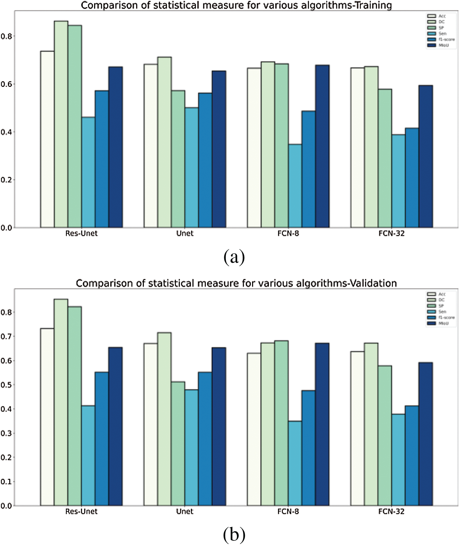
Figure 10: A comparative analysis of statistical measure for various algorithms tested and validated on RIDER dataset (a) training—RIDER Dataset, (b) validation—RIDER dataset
The proposed methodology has been compared with existing models U-Net, FCN8, FCN32 using H&E dataset also. Tab. 3 discusses the comparison of various models and their achieved outcomes using H&E dataset. The ResU-Net achieved training accuracy of 92.12% and validation accuracy of 86.40%. The value for specificity at training time is 94.23% and 88.44% at validation time. Tab. 2 and Fig. 11 depicts the detailed comparison of all statistical measures for the various algorithms used in the analysis for the H&E dataset.
Table 3: Comparative analysis of various models using H&E dataset


Figure 11: A comparative analysis of statistical measure for various algorithms tested and validated on H&E dataset (a) training—H&E Dataset, (b) validation—H&E dataset
The quantitative comparison presents the following conclusions from Tabs. 2 and 3:
1. The segmentation performance of traditional U-Net is better than FCN8, FCN32 with RIDER dataset, but FCN8 outperforms U-Net when applied on H&E dataset.
2. The performance of FCN32 has been on the lower side compared to all the other models in consideration especially for H&E dataset.
In all the evaluation parameters, the proposed ResU-Net outperforms other models, and thus combing the two modules (residual net, batch normalization) has provided a more sophisticated segmentation of breast tumor.
The authors have proposed ResU-Net model for MRI images for breast tumor segmentation and tested on H&E breast histopathology images. The empirical evaluation of the proposed methodology with the existing methodology & H&E dataset shows the robustness of the ResU-Net.
ResU-Net model is proposed for breast tumor segmentation whereas RIDER dataset has been used for experimentation, which is supplemented with ground-reality pictures of MRI scans. In the proposed methodology, a breast tumor image has been segmented as a binary mask from the breast MRI. The performance of the segmentation outputs was evaluated using the six evaluation indices: accuracy, dice coefficient, MIoU, sensitivity, specificity, and F1score. Based on the experimental results, ResU-Net has shown exceptional improvement in breast cancer tumor detection over all the other models into comparison. The accuracy observed for ResU-net is more than the other models. The ResU-net has been able to perform better than the conventional U-net mainly because of the addition of residual networks. The residual network was able to reduce the vanishing gradient problem and help obtain higher accuracy. ResU-net performs better than the FCN’s segmentation model because of three main reasons. First, as it has multiple up-sampling layers, second, as it uses skip connections and concatenates them instead of adding and third, it being its symmetric structure. Finally, it is noteworthy that the approach proposed in this work advances the result towards a more sophisticated tumor segmentation, which is a highly desired result in the diagnostic domain.
Funding Statement: The authors received no specific funding for this study.
Conflicts of Interest: The authors declare that they have no conflicts of interest to report regarding the present study.
1. M. P. Curado. (2011). “Breast cancer in the world: Incidence and mortality,” Salud Pública de México, vol. 53, no. 5, pp. 372–384. [Google Scholar]
2. S. S. Coughlin and D. U. Ekwueme. (2009). “Breast cancer as global health concern,” Cancer Epidemiology, vol. 33, no. 5, pp. 315–318. [Google Scholar]
3. P. Boyle and B. Levin. (2008). World Cancer Report. IARC Press, International Agency for Research on Cancer. [Google Scholar]
4. J. E. Joy, E. E. Penhoet and D. B. Petitti. (2005). Saving Women’s Lives: Strategies for Improving Breast Cancer Detection and Diagnosis. National Research Council, National Academies Press, US. [Google Scholar]
5. A. L. Siu. (2016). “Screening for breast cancer: U.S. preventive services task force recommendation statement,” Annals of Internal Medicine, vol. 164, no. 4, pp. 279–296. [Google Scholar]
6. P. Skaane, A. I. Bandos, R. Gullien, E. B. Eben, U. Ekseth et al. (2013). , “Comparison of digital mammography alone and digital mammography plus tomosynthesis in a population based screening program,” Radiology, vol. 267, no. 1, pp. 47–56. [Google Scholar]
7. D. Saslow, C. Boetes, W. Burke, S. Harms and M. O. Leach. (2007). “American cancer society guidelines for breast screening with MRI as an adjunct to mammography,” CA: A Cancer Journal for Clinicians, vol. 57, no. 25, pp. 75–89. [Google Scholar]
8. W. T. Yang, H. T. Le-Petross, H. Macapinlac, S. Carkaci, M. A. Gonzelez-Angulo et al. (2008). , “Inflammatory breast cancer: PET/CT, MRI, mammography, and sonography findings,” Breast Cancer Research and Treatment, vol. 109, no. 3, pp. 417–426. [Google Scholar]
9. J. H. Chen, B. Feig, G. Agrawal, H. Yu, P. M. Carpenter et al. (2008). , “MRI evaluation of pathologically complete response and residual tumors in breast cancer after neoadjuvant chemotherapy,” Cancer, vol. 112, no. 1, pp. 17–26. [Google Scholar]
10. W. Huang, Y. Chen, A. Fedorov, X. Li, G. H. Jajamovich et al. (2016). , “The impact of arterial input function determination variations on prostate dynamic contrast-enhanced magnetic resonance imaging pharmacokinetic modeling,” Tomography, vol. 2, no. 1, pp. 56–66. [Google Scholar]
11. M. M. Nadrljanski, Z. C. Miloševic, V. Plešinac-Karapandžic and R. Maksimovic. (2013). “MRI in the evaluation of breast cancer patient response to neoadjuvant chemotherapy: Predictive factors for breast conservative surgery,” Diagnostic Interventional Radiology, vol. 19, pp. 463–470. [Google Scholar]
12. V. Badrinarayanan, A. Handa and R. Cipolla. (2017). “SegNet: A deep convolutional encoder–decoder architecture for robust semantic pixel-wise labelling,” IEEE Transactions on Pattern Analysis and Machine Intelligence, vol. 39, no. 12, pp. 2481–2495. [Google Scholar]
13. E. Shelhamer, J. Long and T. Darrell. (2017). “Fully convolutional networks for semantic segmentation,” IEEE Transaction on Pattern Analysis and Machine Intelligence, vol. 39, no. 4, pp. 640–651. [Google Scholar]
14. H. Noh, S. Hong and B. Han. (2015). “Learning deconvolution network for semantic segmentation,” in Proc. of the IEEE Int. Conf. on Computer Vision, Santiago, Chile, pp. 1520–1528. [Google Scholar]
15. L. Li, X. Pan, H. Yang, Z. Liu, Y. He et al. (2020). , “Multi-task deep learning for fine-grained classification and grading in breast cancer histopathological images,” Multimedia Tools & Applications, vol. 79, no. 21–22, pp. 14509–14528. [Google Scholar]
16. A. Rakhlin, A. Shvets, V. Iglovikov and A. A. Kalinin. (2018). “Deep convolutional neural networks for breast cancer histology image analysis,” Lecture Notes in Computer Science, vol. 10882, pp. 737–744. [Google Scholar]
17. B. Kaur, M. Sharma, M. Mittal, A. Verma, L. M. Goyal et al. (2018). , “An improved salient object detection algorithm combining background and foreground connectivity for brain image analysis,” Computers & Electrical Engineering, vol. 71, pp. 692–703. [Google Scholar]
18. P. Herent, B. Schmauch, P. Jehnno, O. Dehaene, C. Saillard et al. (2019). , “Detection and characterization of MRI breast lesions using deep learning,” Diagnostic Interventional Imaging, vol. 100, no. 4, pp. 219–225. [Google Scholar]
19. O. Ronneberger, P. Fischer and T. Brox. (2015). “U-net: Convolutional networks for biomedical image segmentation,” Lecture Notes in Computer Science, vol. 9351, pp. 234–241. [Google Scholar]
20. C. Szegedy, W. Liu, Y. Jia, P. Sermanet, S. Reed et al. (2015). , “Going deeper with convolutions,” in Proc. of the IEEE Computer Society Conf. on Computer Vision and Pattern Recognition, Boston, vol. 07-12-Ju, pp. 1–9. [Google Scholar]
21. A. Krizhevsky, I. Sutskever and G. E. Hinton. (2017). “Imagenet classification with deep convolutional neural networks,” Communications of the ACM, vol. 60, no. 6, pp. 84–90. [Google Scholar]
22. J. Donahue, Y. Jia, O. Vinyals, J. Hoffman, N. Zhang et al. (2014). , “DeCAF: A deep convolutional activation feature for generic visual recognition,” in 31st Int. Conf. on Machine Learning, Berkeley, USA, vol. 2, pp. 988–996. [Google Scholar]
23. K. Simonyan and A. Zisserman. (2014). “Very deep convolutional networks for large-scale image recognition,” arXiv preprint arXiv: 1409.1556. [Google Scholar]
24. J. Chen, L. Yang, Y. Zhang, M. Alber and D. Z. Chen. (2016). “Combining fully convolutional and recurrent neural networks for 3D biomedical image segmentation,” Advances in Neural Information Processing Systems, vol. 29, pp. 3036–3044. [Google Scholar]
25. K. L. Tseng, Y. L. Lin, W. Hsu and C. Y. Huang. (2017). “Joint sequence learning and cross-modality convolution for 3D biomedical segmentation,” in Proc.-30th IEEE Conf. on Computer Vision and Pattern Recognition, Honolulu, Hawaii, pp. 6393–6400. [Google Scholar]
26. Ö. Çiçek, A. Abdulkadir, S. S. Lienkamp, T. Brox and O. Ronneberger. (2016). “3D U-net: Learning dense volumetric segmentation from sparse annotation,” Lecture Notes in Computer Science, vol. 9901, pp. 424–432. [Google Scholar]
27. F. Milletari, N. Navab and S. A. Ahmadi. (2016). “V-net: Fully convolutional neural networks for volumetric medical image segmentation,” in 4th IEEE Int. Conf. on 3D Vision, Stanford, CA, USA, pp. 565–571. [Google Scholar]
28. G. J. Brostow, J. Fauqueur and R. Cipolla. (2009). “Semantic object classes in video: A high-definition ground truth database,” Pattern Recognition Letter, vol. 30, no. 2, pp. 88–97. [Google Scholar]
29. L. Wang, B. Platel, T. Ivanovskaya, M. Harz and H. K. Hahn. (2012). “Fully automatic breast segmentation in 3D breast MRI,” in Proc.-Int. Symp. on Biomedical Imaging, Barcelona, Spain, pp. 1024–1027. [Google Scholar]
30. M. I. Daoud, M. M. Baba, F. Awwad, M. Al-Najjar and E. S. Tarawneh. (2012). “Accurate segmentation of breast tumors in ultrasound images using a custom-made active contour model and signal-to-noise ratio variations,” in 8th Int. Conf. on Signal Image Technology and Internet Based Systems, Naples, Italy, pp. 137–141. [Google Scholar]
31. D. C. Cireşan, A. Giusti, L. M. Gambardella and J. Schmidhuber. (2012). “Deep neural networks segment neuronal membranes in electron microscopy images,” Advances in Neural Information Processing Systems, vol. 4, pp. 2843–2851. [Google Scholar]
32. J. A. Rosado-Toro, T. Barr, J. P. Galons, M. T. Marron, A. stopeck et al. (2015). , “Automated breast segmentation of fat and water MR images using dynamic programming,” Academic Radiology, vol. 22, no. 2, pp. 139–148. [Google Scholar]
33. A. Vignati, V. Giannini, M. De Luca, L. Morra, D. Persano et al. (2011). , “Performance of a fully automatic lesion detection system for breast DCE-MRI,” Journal of Magnetic Resonance Imaging, vol. 34, no. 6, pp. 1341–1351. [Google Scholar]
34. G. Piantadosi, M. Sansone and C. Sansone. (2018). “Breast segmentation in MRI via U-net deep convolutional neural networks,” in Proc.-24th Int. Conf. on Pattern Recognition, Beijing, China, pp. 3917–3922. [Google Scholar]
35. F. Khalvati, C. Gallego-Ortiz, S. Balasingham and A. L. Martel. (2015). “Automated segmentation of breast in 3-D MR images using a robust atlas,” IEEE Transaction Medical Imaging, vol. 34, no. 1, pp. 116–125. [Google Scholar]
36. V. Giannini, A. Vignati, L. Morra, D. Persano, D. Brizzi et al. (2010). , “A fully automatic algorithm for segmentation of the breasts in DCE-MR images,” in Int. Conf. of the IEEE Engineering in Medicine and Biology Society, Buenos Aires, Argentina, pp. 3146–3149. [Google Scholar]
37. G. Piantadosi, M. Sansone, R. Fusco and C. Sansone. (2020). “Multi-planar 3D breast segmentation in MRI via deep convolutional neural networks,” Artificial Intelligence in Medicine, vol. 103, pp. 101781. [Google Scholar]
38. M. H. Aghdam and P. Kabiri. (2016). “Feature selection for intrusion detection system using ant colony optimization,” International Journal of Network Security, vol. 18, no. 3, pp. 420–432. [Google Scholar]
39. A. Gubern-Mérida, M. Kallenberg, R. Martí and N. Karssemeijer. (2012). “Segmentation of the pectoral muscle in breast MRI using atlas-based approaches,” Lecture Notes in Computer Science, pp. 371–378. [Google Scholar]
40. M. Havaeai, A. Davy, D. F. Warde, A. Biard, A. Courville et al. (2017). , “Brain tumor segmentation with deep neural networks,” Medical Image Analysis, vol. 35, pp. 18–31. [Google Scholar]
41. A. Zotin, K. Simonov, M. Kurako, Y. Hamad and S. Kirillova. (2018). “Edge detection in MRI brain tumor images based on fuzzy C-means clustering,” Procedia Computer Science, vol. 126, pp. 1261–1270. [Google Scholar]
42. M. Mittal, A. Verma, I. Kaur, B. Kaur, M. Sharma et al. (2019). , “An efficient edge detection approach to provide better edge connectivity for image analysis,” IEEE Access, vol. 7, pp. 33240–33255. [Google Scholar]
43. J. Deng, W. Dong, R. Socher, L. J. Li, K. Li et al. (2009). , “ImageNet: A large-scale hierarchical image database,” in IEEE Conf. on Computer Vision and Pattern Recognition, Miami, FL, USA, pp. 248–255. [Google Scholar]
44. K. He, X. Zhang, S. Ren and J. Sun. (2016). “Deep residual learning for image recognition,” in Proc. of the IEEE Computer Society Conf. on Computer Vision and Pattern Recognition, Las Vegas, pp. 770–778. [Google Scholar]
45. J. Canny. (1986). “A computational approach to edge detection,” IEEE Transactions on Pattern Analysis and Machine Intelligence, vol. 8, no. 6, pp. 679–698. [Google Scholar]
46. M. Mittal, L. M. Goyal, S. Kaur, I. Kaur, A. Verma et al. (2019). , “Deep learning based enhanced tumor segmentation approach for MR brain images,” Applied Soft Computing, vol. 78, pp. 346–354. [Google Scholar]
47. L. C. Chen, G. Papandreou, K. Murphy and A. L. Yuille. (2014). “Semantic image segmentation with deep convolutional nets and fully connected Crfs,” arXiv preprint arXiv: 1412.7062. [Google Scholar]
48. C. García and J. A. Moreno. (2004). “Kernel based method for segmentation and modeling of magnetic resonance images,” Lecture Notes in Artificial Intelligence, vol. 3315, pp. 636–645. [Google Scholar]
49. S. Kaur, R. K. Bansal, M. Mittal, L. M. Goyal, I. Kaur et al. (2019). , “Mixed pixel decomposition based on extended fuzzy clustering for single spectral value remote sensing images,” Journal of the Indian Society Remote Sensing, vol. 47, no. 3, pp. 427–437. [Google Scholar]
50. Z. Zhang, Q. Liu and Y. Wang. (2018). “Road extraction by deep residual U-net,” IEEE Geoscience and Remote Sensing Letters, vol. 15, no. 5, pp. 749–753. [Google Scholar]
51. B. Kayalibay, G. Jensen and P. van der Smagt. (2017). “CNN-based segmentation of medical imaging data,” arXiv preprint arXiv: 1701.03056. [Google Scholar]
52. Z. Zhuang, N. Li, A. N. J. Raj, V. G. V. Mahesh and S. Qiu. (2019). “An RDAU-NET model for lesion segmentation in breast ultrasound images,” PLoS One, vol. 14, no. 8, pp. e0221535. [Google Scholar]
53. H. Chen, Q. Dou, L. Yu and P. A. Heng. (2018). “VoxResNet: Deep voxelwise residual networks for volumetric brain segmentation from 3D MR images,” Neuroimage, vol. 170, pp. 446–455. [Google Scholar]
54. Data from RIDER-breast-MRI. (2015). “The cancer imaging archive,” . https://wiki.cancerimagingarchive.net/display/Public/RIDER+Breast+MRI. [Google Scholar]
55. J. C. Reinhold, B. E. Dewey, A. Carass and J. L. Prince. (2019). “Evaluating the impact of intensity normalization on MR image synthesis,” in Proc. SPIE 10949, Medical Imaging: Image Processing, San Diego, California, United States, vol. 10949. [Google Scholar]
56. A. Dosovitskiy, J. T. Springenberg and T. Brox. (2013). “Unsupervised feature learning by augmenting single images,” arXiv preprint arXiv: 1312.5342. [Google Scholar]
57. R. Wu, S. Yan, Y. Shan, Q. Dang and G. Sun. (2015). “Deep Image: Scaling up image recognition,” arXiv preprint, no. 8, arXiv preprint arXiv: 1501.02876. [Google Scholar]
58. S. Ioffe and C. Szegedy. (2015). “Batch normalization: Accelerating deep network training by reducing internal covariate shift,” in 32nd Int. Conf. on Machine Learning, vol. 1, pp. 448–456. [Google Scholar]
59. D. P. Kingma and J. L. Ba. (2017). “Adam: A method for stochastic optimization,” in Proceeding ICLR, pp. 1–15. [Google Scholar]
60. L. R. Dice. (1945). “Measures of the amount of ecologic association between species,” Ecology, vol. 26, no. 3, pp. 297–302. [Google Scholar]
61. B. Hariharan, P. Arbeláez, R. Girshick and J. Malik. (2014). “Simultaneous detection and segmentation,” Lecture Notes in Computer Science, vol. 8695, pp. 297–312. [Google Scholar]
62. UCSB Bio-segmentation dataset, https://bioimage.ucsb.edu/research/bio-segmentation. [Google Scholar]
 | This work is licensed under a Creative Commons Attribution 4.0 International License, which permits unrestricted use, distribution, and reproduction in any medium, provided the original work is properly cited. |