DOI:10.32604/cmc.2021.013164
| Computers, Materials & Continua DOI:10.32604/cmc.2021.013164 | |
| Article |
A Cell-Based Smoothed Finite Element Method for Modal Analysis of Non-Woven Fabrics
12C2T—Centro de Ciência e Tecnologia Têxtil, Departamento de Engenharia Têxtil, Universidade do Minho, Campus de Azurém, Guimarães, 4804-533, Portugal
2CMEMS-UMinho, Departamento de Engenharia Mecânica, Universidade do Minho, Campus de Azurém, Guimarães, 4804-533, Portugal
3Department of Computer Science, Universidade da Beira Interior, Convento de Sto. António,, Covilhã, 6201-001, Portugal
4Instituto de Telecomunicações, R. Marquês de Ávila e Bolama, Covilhã, 6201-001, Portugal
*Corresponding Author: Nguyễn T. Quyền. Email: quyen@2c2t.uminho.pt
Received: 30 August 2020; Accepted: 30 November 2020
Abstract: The combination of a 4-node quadrilateral mixed interpolation of tensorial components element (MITC4) and the cell-based smoothed finite element method (CSFEM) was formulated and implemented in this work for the analysis of free vibration and unidirectional buckling of shell structures. This formulation was applied to numerous numerical examples of non-woven fabrics. As CSFEM schemes do not require coordinate transformation, spurious modes and numerical instabilities are prevented using bilinear quadrilateral element subdivided into two, three and four smoothing cells. An improvement of the original CSFEM formulation was made regarding the calculation of outward unit normal vectors, which allowed to remove the integral operator in the strain smoothing operation. This procedure conducted both to the simplification of the developed formulation and the reduction of computational cost. A wide range of values for the thickness-to-length ratio and edge boundary conditions were analysed. The developed numerical model proved to overcome the shear locking phenomenon with success, revealing both reduced implementation effort and computational cost in comparison to the conventional FEM approach. The cell-based strain smoothing technique used in this work yields accurate results and generally attains higher convergence rate in energy at low computational cost.
Keywords: Mindlin–Reissner theory of plates; shear-locking; gradient/strain smoothing technique; non-woven fabric
Thin shells are of paramount importance in many engineering applications, namely in civil, mechanical, textile, aeronautical and maritime areas. Shell structures can be found in large-span roofs, liquid reservoirs and arch domes in civil engineering applications. Shells can also be used in pressure vessels, pipes and turbine disks, as examples of mechanical engineering applications. Non-woven fabrics are examples found in many textile products that can be identified in ceiling covering panels, roof linings for automotive interiors and geotextile mats [1,2]. Fuselages, missiles and ship hulls are important examples of both aeronautical and marine engineering industries. The above referred examples represent just a few structural applications that employ shells whose vibrational actions and buckling are important aspects to take into account by engineers and product development designers.
Mathematically, a shell structure can be analysed as a plate structure (or sheet) with curved middle surface upon different boundary conditions. Plates can typically endure transverse loads resulting in bending. Shells, on the other hand, withstand loads in any direction.
The formulations currently employed to describe the mechanical behaviour of shells use: (A) curved shells elements, which are established on the basis of the general shell theory [3]; (B) degenerated shell elements, derived from the three dimensional solid theory [4]; and (C) flat shell elements, which combine a plane membrane element and a plate bending element [5]. Due to their more straightforward mathematical formulation and lower computational costs, flat shell elements are commonly used in many numerical computations to analyse the mechanical behaviour of thin structures, even for complex loading and imposed boundary conditions [6]. A relevant aspect that affects the mechanical behaviour of flat shell elements regards the thickness and curvature of their mid-surface. Concerning their thickness, these elements can be classified as either thin or thick. The available mathematical approach to characterize thin shell elements is based on Kirchoff–Love theory, for which the transverse shear deformations are considered negligible. For the thick ones, the Mindlin theory is employed, which takes into account the transverse shear deformations that can be affected by a well-known phenomenon referred to as shear locking. This numerical setback is detected when the thickness-to-length ratio becomes large, being characterized by a spurious stiffness due to the existence of a parasitic shear deformation energy. Consequently, the numerical solutions turn inaccurate and impractical to describe stress and strain fields developed in the physical domain. To prevent this phenomenon, several numerical approaches have been developed, contributing to solve this problem in different degrees of success. The reduced and selective integration scheme is one of the most appropriate technique to mitigate the shear locking phenomenon. As proposed by Hughes et al. [7], the strain energy was separated in two parts, shear and bending, whose different strain energies were obtained employing a different integration scheme. Such reduced integration technique leads to numerical instabilities due to rank deficiency, which yields in zero-energy modes [8,9]. Other techniques are the assumed strain method [10], the field redistributed shape functions [11], the mixed interpolation of tensorial components (MITC) technique [8,12,13] and the smoothed finite element method (SFEM) [14,15].
The MITC allows employing a full quadrature (or integration) in the components of the stiffness matrix, thus eliminating detected inconsistencies of the used interpolation functions for displacements and strains without considering the assumption of additional degrees of freedom. This is the reason why the MITC method has recently been receiving much attention, in particular for the implementation of shell elements and locking-free plates [16–18]. The theoretical fundaments of the MITC shell elements are well stablished in the literature [8,19–23], with numerous test problems duly verified numerically [20]. However, no study has been conducted to analyse convergence regarding the effect of shell thickness for different edge boundary conditions.
The cell-based smoothed finite element method (CSFEM), a typical S-FEM model proposed by Nguyen-Xuan et al. [14], showed that the strain smoothing operation performed on the strain matrices (i.e., improved solutions for lower ordered elements) allows to gain robustness of element performance against geometric distortion, while providing accurate results and high convergence rate in energy, at low computational cost [24]. This is the solution for poor performance of elements affecting many standard FEM computations involving irregular (intricate) geometries that lies in the required mapping from the parental and the physical domain [24]. Also, contrarily to Gauss integration techniques (in standard FEM), SFEM can evaluate strain fields directly at each discrete point in cell boundaries. These characteristics are more flexible in regards to the selection of element type within the integration domain and corresponding allowed node location. This method renders possible to improve the adaptability of SFEM meshes comparatively to standard FEM approaches.
In the SFEM approach, the strain values in an element are modified by smoothing the compatible strain fields over smoothing domains, which originates important softening results. This technique is now known as the cell-based FEM, or simply CSFEM [14,24–28].
In this work a combination of the 4-node quadrilateral MITC element (MITC4) and cell-based FE method (CSFEM) was formulated and implemented (in Python) to analyse the mechanical response of a rectangular non-woven fabric structure under free vibration and unidirectional buckling. The original formulation of CSFEM was modified in the sense that the unit outward normal vectors are substituted by outward normal vectors, which allowed to remove the integral operator in the strain smoothing method. A wide range of values for the thickness-to-length ratio was analysed considering different edge boundary conditions and various domain discretization in standard numerical examples to demonstrate the robustness of the developed numerical formulation. The achieved results were compared with analytical and standard FEM approaches, with significant gains in implementation and computational costs.
Consider the linear elastic domain  contained within the so-called Lipschitz-continuous boundary
  (Fig. 1), under surface-traction
  on the boundary
  , and body force
  within the domain
  . Besides the Dirichlet boundary conditions
  applied in the domain
  (i.e., fixed), the elastic domain
  is also subjected to the Neumann boundary conditions
  in
in  , such that
  , with
  .
.
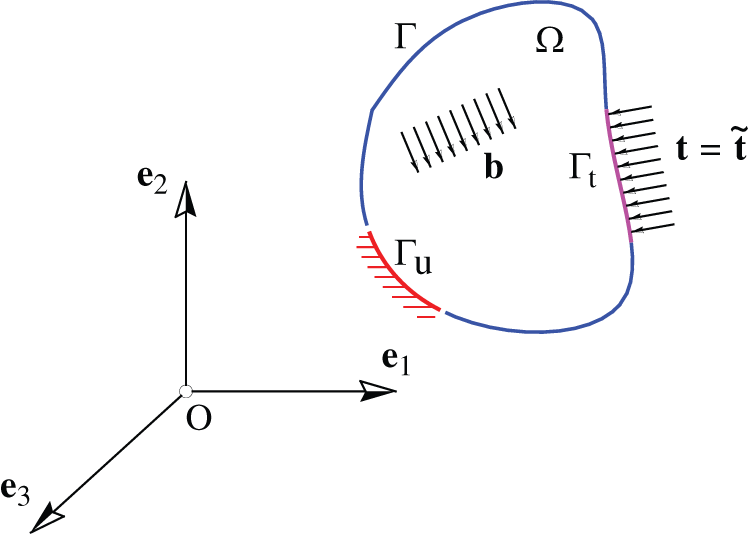
Figure 1: Elastic domain  of an arbitrary shape subjected to traction
  and distributed body forces
Assume that the displacements induced in the domain  are the state variables of this problem (considering that
  does not include its boundary
  ). Upon small deformation (i.e., elastic problems), the strain energy is simply a function of the displacement
  , being determined as follows,

with  standing for the Cauchy stress tensor and
  for the strain tensor, defined as

which is known as the compatibility equation.  is the gradient vector. Stress–strain components (i.e., the constitutive equations) are established as

being  the elasticity tensor (see [29] for plane stress analysis).
The local equations of equilibrium for a static problem is formulated through,

While the boundary conditions in terms of stress dictate

with  representing the outward unitary normal vector to
  illustrated in Fig. 1. Eq. (4) is frequently referred to as the strong form, because the differential equation must be satisfied at each point of the domain
  . In addition, Eq. (4) must provide a solution
  that is smooth enough such that its second-order derivatives are continuous, i.e.,
  . In this sense, although Eq. (4) only considers the existence of a divergence operator, being a first-order derivative, the continuous mechanics problem has second-order derivatives, since strain implies derivatives of displacements (Eq. (2)).
The purpose of the so-called boundary-value problem is to identify the displacement value  that satisfies Eqs. (4) and (5) within
  and
and  , respectively, as well as the Dirichlet boundary condition (i.e.,
  on
on  ). If the applied forces lead to deformations in the direction of those forces, then one can conclude that the work is performed by those forces. Such work is calculated through

which contemplates the work performed by the body forces  and the work resulting from the applied surface-traction
  . Upon the application of an external concentrated load
  (not represented in Fig. 1), Eq. (6) must include the Dirac delta measure. Hence, the potential energy stored in the elastic domain is computed from the difference between the elastic strain energy (Eq. (1)) and the work performed by the applied loads (Eq. (6)),

For all displacements that satisfy the boundary conditions, i.e., those that are adequate to the boundary-value problem (Eqs. (4) and (5)), the potential energy  in Eq. (7) is stationary on the solution spaces

which are used in the following to get a generalized solution to the differential equation through the principle of minimum total potential energy. Thus, for the solution  that minimizes
  in Eq. (7),
  in Eq. (8) must be extended so that the potential energy
  can be estimated correctly. For this reason,
  is known as the space of finite energy or space of kinematically admissible displacements, being defined as

with  representing the Sobolev space of unitary order [30].
The principle of minimum potential energy formulated in Eq. (7) requires attaining a stationary condition for the potential energy, whose principle is related to the variational formulation. Hence, consider that the displacement  is the solution of the problem that allows minimizing the total potential energy, and assume that the functional
  is defined in
  . Therefore, if the quantity

exists, then it refers to the first variation of  at
at  in the same direction of
  . Thus, if this limit exists within the domain
  , then it is possible to conclude that
  is differentiable (Fréchet concept) at
  . Also, if a functional admits a first variation, then one can establish a quantitative criterion for its minimization. In this respect, suppose that
  is defined such that

then  is said to minimize
  over
over  . Also, if Eq. (11) is valid for
  that respects
  , for some
  , hence
  presents a relative minimum value at
  .
.
According to Eq. (11), for  and for any appropriately small value of
  , if
, if  has a relative minimum at
  , then one can establish

which means that for fixed values of  and
and  , the real value function on parameter
  , i.e.,
  , leads to a minimum value at point
  . Hence, one can conclude that if the functional
  admits a first variation, then the quantity
  is a differentiable function of
  . Consequently, a necessary condition for a minimum value of
  at
at  is
is

which, as mentioned above, represents a variation of  at
at  in the direction of
  . Eq. (13) establishes the principle of minimum potential energy for any kinematically admissible displacement value
  .
.
Considering Eq. (7), a first variation of  establishes,

which configures the variational equation of the structural problem. The first term of Eq. (14) is related with the strain energy  and the constitutive equations (i.e., Eqs. (1) and (3), respectively). Therefore, upon substitution yields

In this equation,  is the energy-bilinear form, since it is linear in each of its arguments
  and
and  . One can conclude that
  is made the same as
  in Eq. (2), by substituting
  into
into  , which makes
  symmetric with respect to their arguments. In regards to the work performed by the applied load, Eq. (6) allows to establish

with  standing for the load-linear form. This formulation only regards conservative loads, which makes the functional
  independent of the displacement. Therefore, one can rewrite Eq. (14) as follows,

This equation has a unique solution,  , if the load-linear form in right-hand side is continuous in the space,
  , and if energy-bilinear form in the left-hand side is positive definite on
  . Then, if a solution exists to the differential equation, one can conclude that there will be a solution for the variational equation, Eq. (16). Additionally, if the applied surface-traction
  (i.e., distributed function) is a Dirac delta measure, i.e., is a concentrated load, then Eq. (4) may not have a solution. Besides that, the variational equation (Eq. (16)) still has a solution, known as generalized solution.
Consider  at the configuration domain (
 ) forming the mid-surface of the Mindlin-Reissener shell described by,

Fig. 2 shows an anisotropic shell, for which the analysis of the membrane deformations can be performed. In such domain the uncoupling of bending and shear deformations is feasible. Therefore, the displacement assumption turns,

with u0, v0 and w0 standing, respectively, for the membrane displacement components along x, y and z directions.
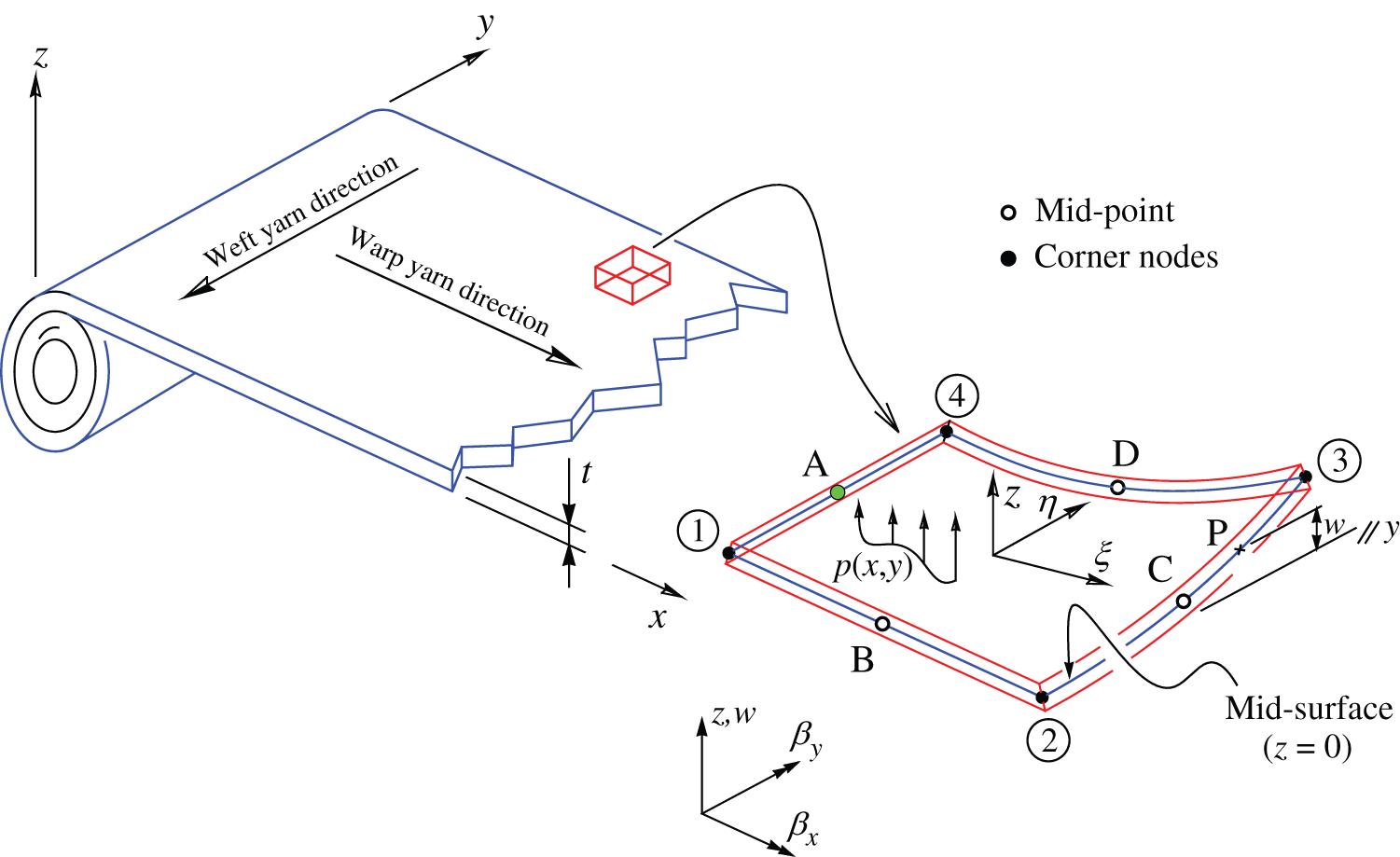
Figure 2: Moderately thick sheet fabric showing characteristic dimensions
The matrices of membrane strain  and curvature strain
  are calculated from the corresponding 2D differential operators,

and the displacement components 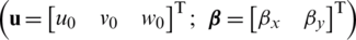 , turning,

while the membrane strain is defined by

Considering Eq. (1), as the shell is submitted to pre-buckling in-plane stresses (i.e.,  ,
,  and
and  ), the geometric elastic strain energy gives

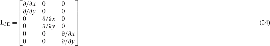
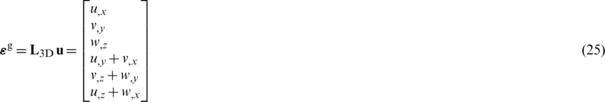
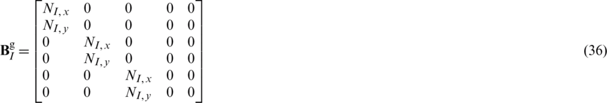
being  defined as the geometrical strain matrix, which is evaluated as a function of the 3D differential operator (
 ),
),
and, based on the of the displacement assumption (Eq. (19)),
The pre-buckling in-plane stress is expressed as,

being,

2.2 Finite Element Formulation
The general displacement solution 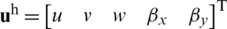 of the finite element model for the shell is defined as follows,
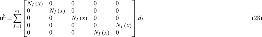
with nI stands for the total number of nodes of the finite element,  the bilinear shape functions related to node I, and
 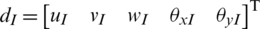 the nodal degrees of freedom of
  , also associated to node I. Let
  be the number of nodes of the element. Then, the approximate form of the membrane strain field is established as follows,

in which,

The discrete curvature field  , the shear strain field
  , and the geometrical strain field are expressed by,


with,


and
The nodal unknowns can be expressed by considering the discretized system of equations of the Mindlin/Reissner theory for shells. Therefore, using the FEM procedure for a static analysis, yields

with the stiffness at the element domain  given by

and the corresponding load components defined,

considering  the prescribed boundary load components. For vibration analysis, the discretized governing equation is

with  standing for the global stiffness matrix and
  for the natural frequency of the mechanical system.
  represents the global mass matrix which is established through the assembly of the element matrix, as follows

To analyse the buckling effect, the discretized governing equation is

with  representing the critical buckling load, and

where for the present case,  .
.
2.3 Mixed Interpolation of Tensorial Component
Mindlin–Reissner type plate elements are affected by an intrinsic limitation known as locking, i.e., the presence of spurious stresses in plates of small thickness, which can occur in the last term of Eq. (38). This numerical non-conformity is a characteristic of low-order finite elements, which is solved by employing higher-order elements [31]. Early methods to try tackling the locking phenomenon in thin plates employed reduced integration, or a selective reduced integration [32]. By splitting the strain energy into a shear part and a bending part, it turns possible to apply different integration rules for each loading component. This method leads to an instability owing to rank deficiency, which results in zero-energy modes that can be solved by an hourglass control [27]. Transverse shear locking, a well-known type of locking induced by transverse forces under bending and large oscillating shear/transverse forces, can benefit from a simple smoothing procedure to drastically improve the results [31]. Nevertheless, shell elements fail the completeness condition [27], known as patch test [33], and exhibit an instability owed to rank deficiency [31]. To solve this important limitation, independent interpolation fields in the natural coordinate system are performed to obtain the approximation of the shear strains [10] by means of

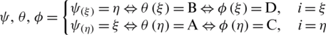
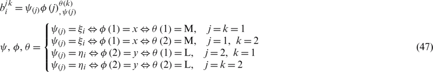
Shear strain components in the natural coordinate system  (
( ) are obtained considering the mid-point edge nodes of the element shown in Fig. 2 (i.e., nodes A, B, C and D), by applying a permutation index notation

(which allows obtaining:  and
and  ).
).  stands for the Jacobian matrix. A convenient way to eliminate the parasitic transverse shear strains in the element is to place the sampling points at
  , in the case that the shell is submitted to bending relative to the
  -axis. It should be noted that the shear component
  varies linearly along the
  -direction. With the purpose to retain a linear variation of the component
  along
along  -direction, two sampling points were chosen, A and C (Fig. 2), and the pattern coordinates
  ,
,  and
and  ,
,  . Similarly, a linear variation of the component
  is retained along
  -direction, by choosing the points B and D, and the coordinates
  ,
,  and
and  ,
,  . Considering the shear values
  ,
,  and
and  ,
,  , and considering the way that the discretized fields
  were made, the shear matrix turns

with
considering that  ,
,  and
and 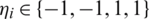 .
.
The modification of the compatible strain fields  ,
,  ,
,  (i.e., Eqs. (29), (31) and (33), respectively) can be directly evaluated using the assumed displacement field. The smoothed strain field
  at
at  can be computed using the integral approximation technique [34] in the following way,

 is a smoothing function associated with
  , that fulfils the following basic condition

For a sake of simplicity,  can be defined using the Heaviside-type smoothing function,

in which  represents the area of the smoothing cell (Fig. 3),
  . Combining Eqs. (50) and (48), and upon consideration of the divergence theorem, the smoothed strain field in
  yields,

being ni and nj the Cartesian components of the unit outward normal vector on the cell boundary 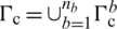 (see Fig. 3d). By applying the smoothed operator (Eq. (48)), to Eqs. (29), (31) and (33), it may be established


with  ,
,  and
and  standing for the outward normal vectors. Hence, the relationship between the strain fields and nodal displacement components can be evaluated by,


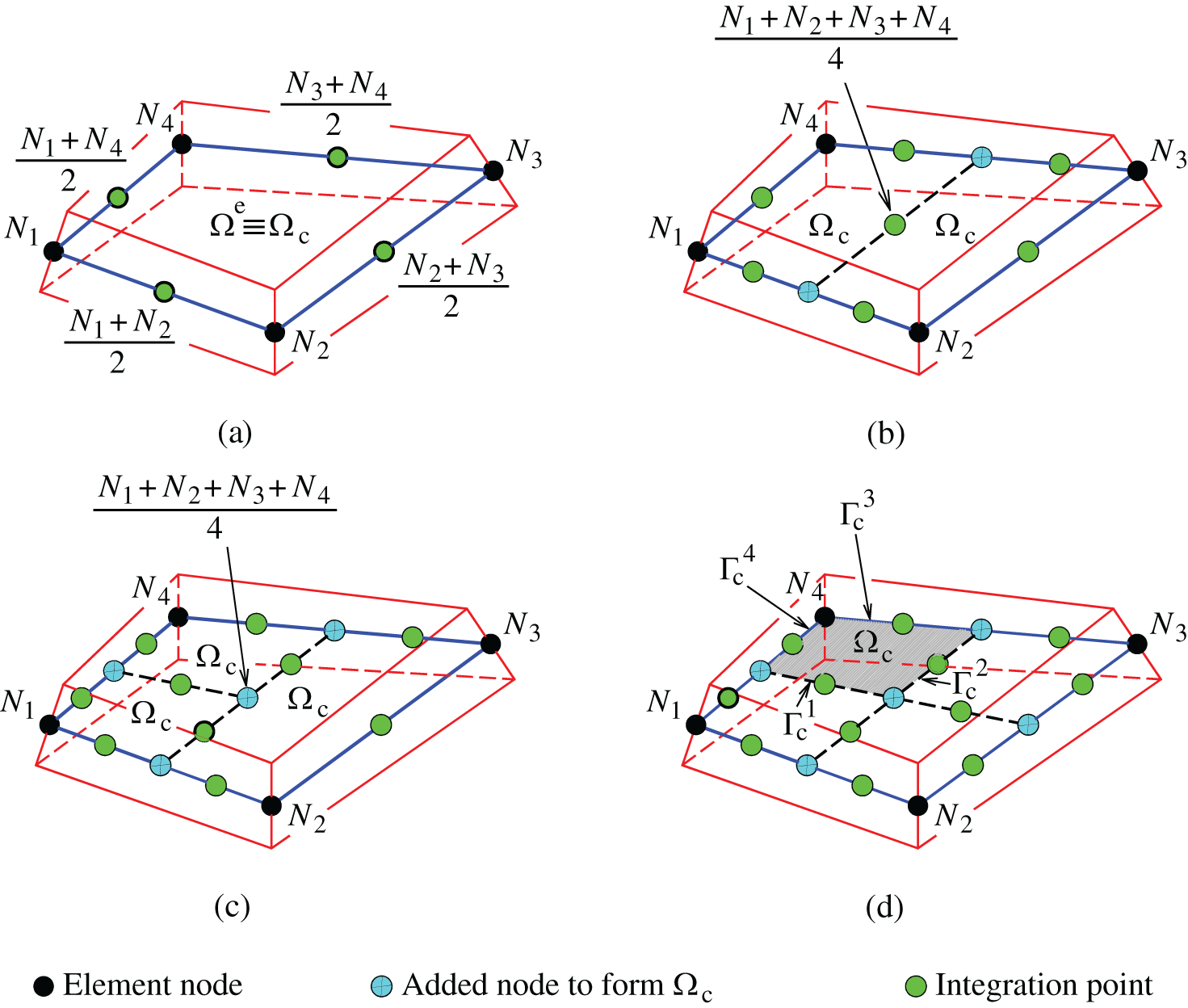
Figure 3: Division of  into
into  cells to form
  domains
It should be noted that the strains are constant within the domain of each cell  , while the matrices of non-local strain displacement are defined as,


It should be noted that the integration points in Fig. 3 are used to evaluate Eqs. (58)–(60), along each segment of  . Therefore, Eq. (38) becomes

where,


The geometrical element stiffness matrix can be defined as follows,

Two examples have been analysed regarding the application of the CS-FEM and MITC4 formulations. The performed analyses comprise the problematic of free vibration and buckling of a square non-woven fabric sheet (Fig. 4a) employing a mesh regularly structured (Fig. 4b) in the range of 10 to 35 elements. The adopted values for the thickness-to-length ratio (t/L) are the ones given in Tabs. 1–16, together with the used configuration (i.e., number of elements  and corresponding number of nodes, Q4), and the number of smoothing cells (sub-cells
  ). Additionally, the used boundary conditions, i.e., fully simply supported (SSSS) and fully clamped (CCCC), as well as SCSC and CCCF situations (F standing for free side) are identified. Values of non-dimensional natural frequency
  and normalized eigenvalues
  were obtained for CS-FEM, MITC and FEM approaches, considering the shear factor corrections k shown in Tabs. 1–16. Also, values of
  and
and  were provided in those Tables for comparison purposes (analytical or/and numerical solutions). Good agreement is observed with mixed interpolation of tensorial components (MITC), finite element method (FEM), analytical solution, and closed form results, which indicate both the validity and accuracy of the developed approach. Furthermore, carpet plots are shown in Figs. 5–20, to allow perceiving, respectively, how
  and
and  evolve within the sheet domain when the used number of elements is set to
  . Tabs. 13–16, together with Figs. 17–20 reveal that buckling load decreases with the thickness-to-length ratio (t/L) increase.
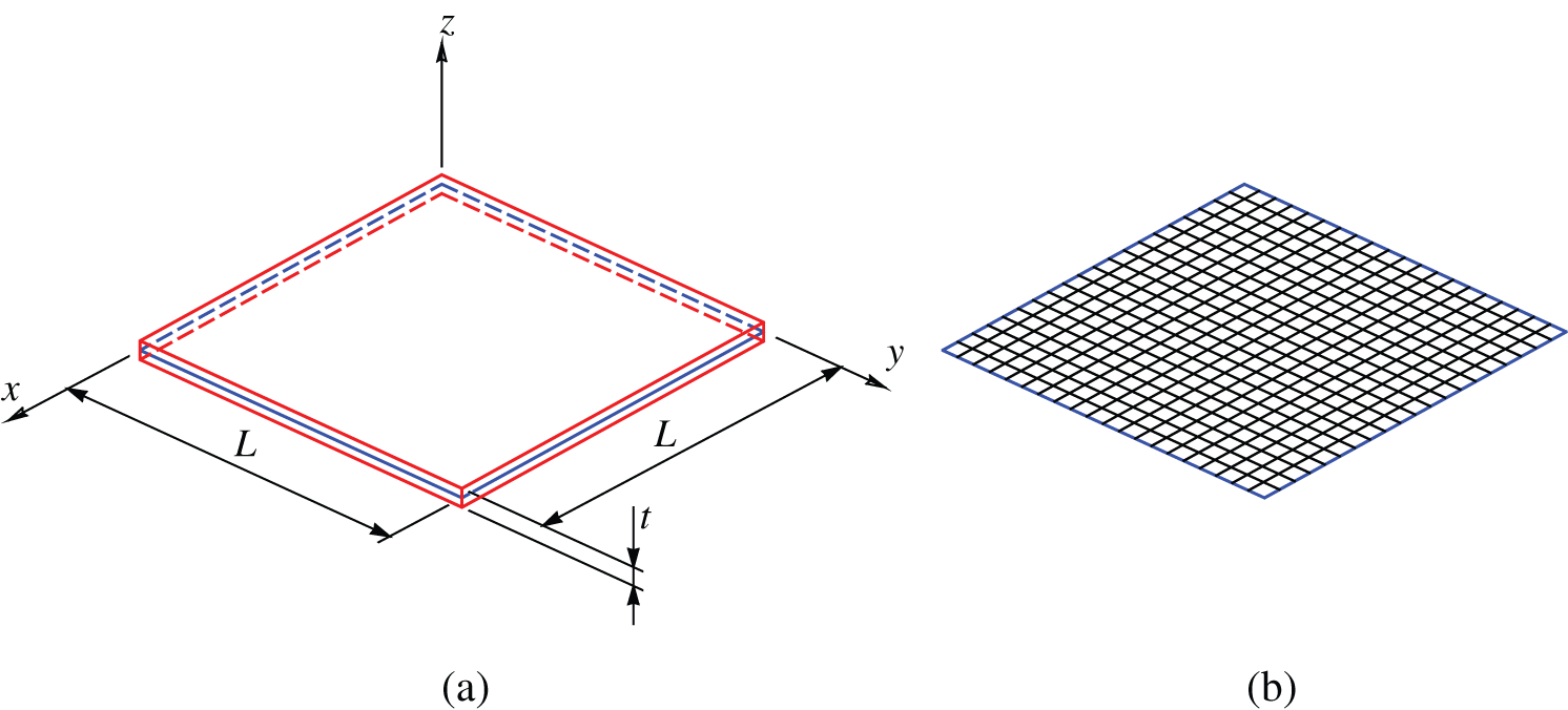
Figure 4: Illustration of (a) a thin square non-woven fabric sheet and (b) a Mindlin sheet  Q4 mesh employed in free vibration and buckling numerical analyses
Table 1: Numerical results of non-dimensional natural frequency  for a CCCC sheet considering t/L = 0.01, k = 0.8601 and
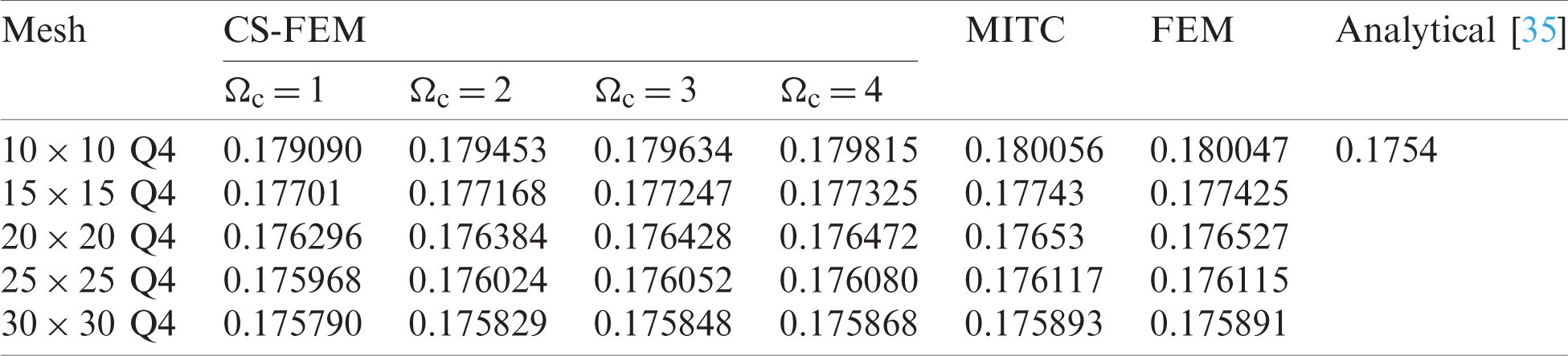
Table 2: Numerical results of non-dimensional natural frequency  for a SSSS sheet considering t/L = 0.01, k = 0.8333 and
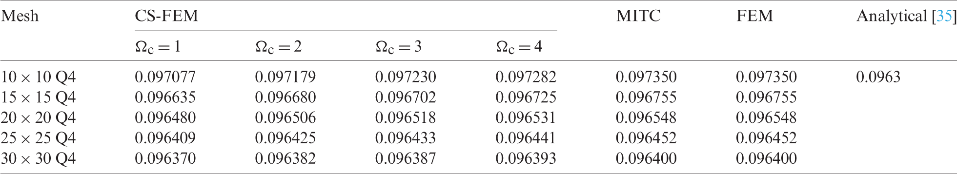
Table 3: Numerical results of non-dimensional natural frequency  for a CCCC sheet considering t/L = 0.1, k = 0.8601 and
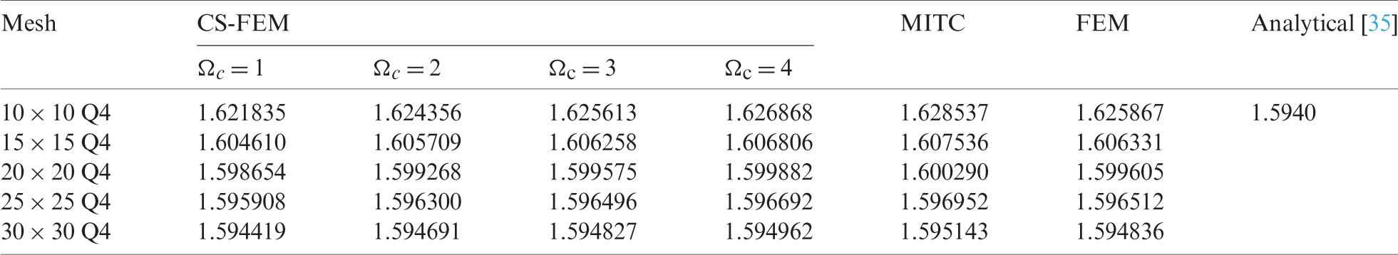
Table 4: Numerical results of non-dimensional natural frequency  for a SSSS sheet considering t/L = 0.1, k = 0.8333 and
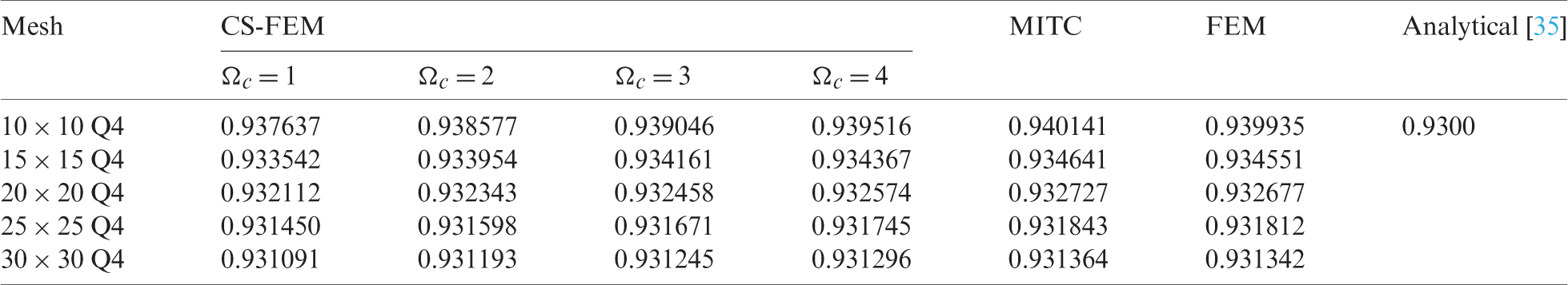
Table 5: Numerical results of non-dimensional natural frequency  for a SSSS sheet considering t/L = 0.1, k = 0.8333 and
  (using a mesh:
  )
)

Table 6: Numerical results of non-dimensional natural frequency  for a SSSS sheet considering t/L = 0.01, k = 0.8333 and
  (using a mesh:
  )
)
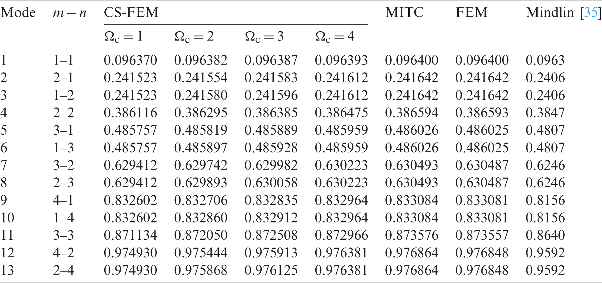
Table 7: Numerical results of non-dimensional natural frequency  for a CCCC sheet considering t/L = 0.1, k = 0.8601 and
  (using a mesh:
  )
)
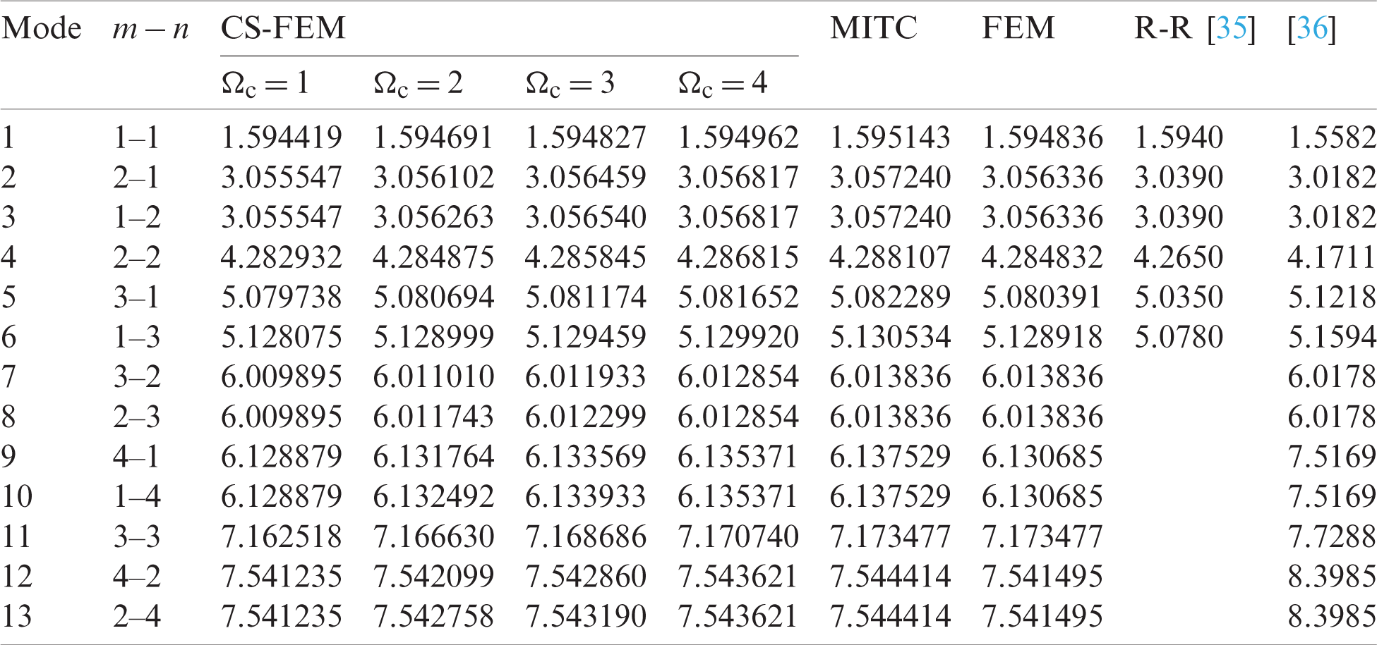
Table 8: Numerical results of non-dimensional natural frequency  for a CCCC sheet considering t/L = 0.01, k = 0.8601 and
  (using a mesh:
  )
)
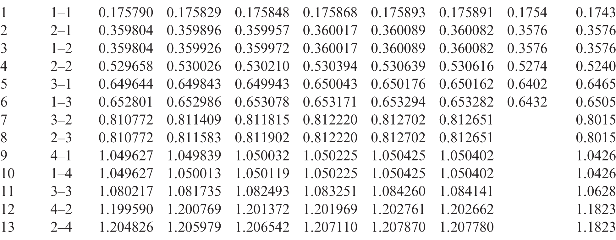
Table 9: Numerical results of non-dimensional natural frequency  for a SCSC sheet considering t/L = 0.1, k = 0.8222 and
  (using a mesh:
  )
)
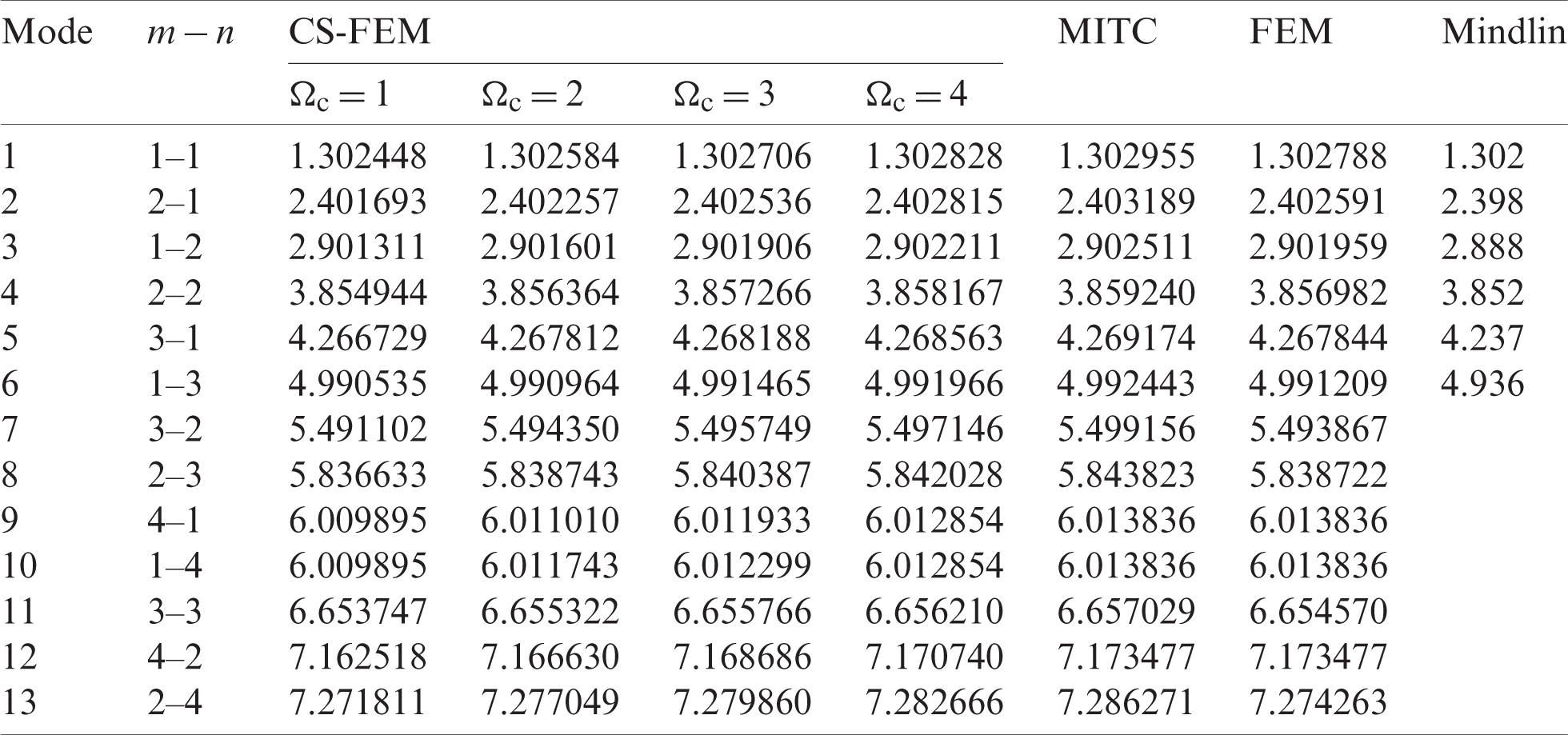
Table 10: Numerical results of non-dimensional natural frequency  for a SCSC sheet considering t/L = 0.01, k = 0.8222 and
  (using a mesh:
  )
)
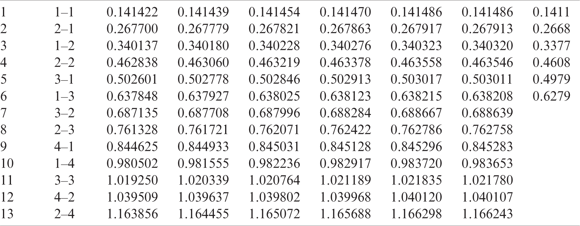
Table 11: Numerical results of non-dimensional natural frequency  for a CCCF sheet considering t/L = 0.1, k = 0.8601 and
  (using a mesh:
  )
)
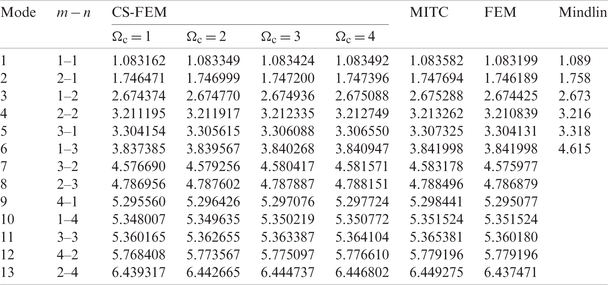
Table 12: Numerical results of non-dimensional natural frequency  for a CCCF sheet considering t/L = 0.01, k = 0.8601 and
  (using a mesh:
  )
)
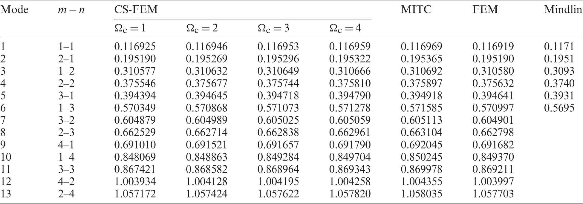
Table 13: Normalized eigenvalues for buckling ( ) considering a SSSS sheet with t/L = 0.001, k = 0.8333 and
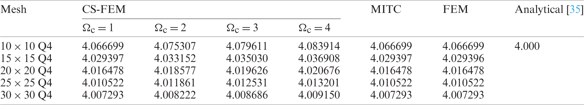
Table 14: Normalized eigenvalues for buckling (. .) considering a SSSS sheet with t/L = 0.05, k = 0.8333 and
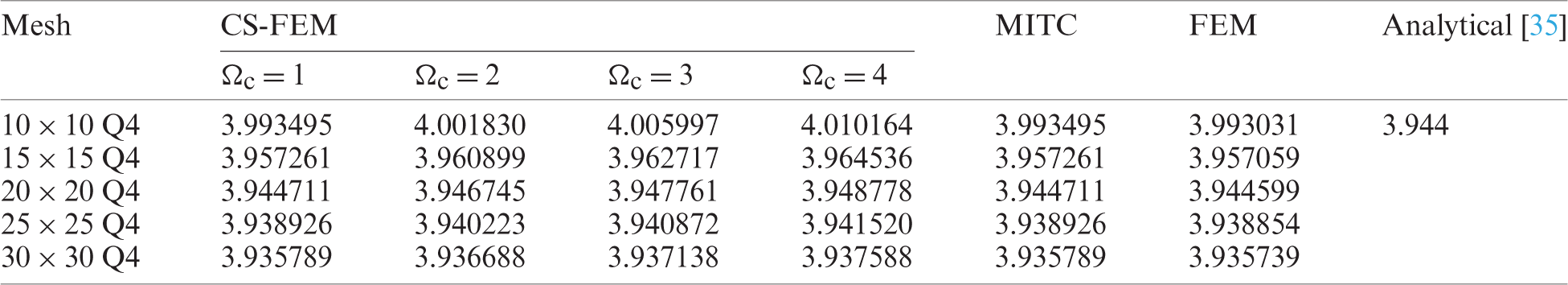
Table 15: Normalized eigenvalues for buckling ( ) considering a SSSS sheet with t/L = 0.1, k = 0.8333 and
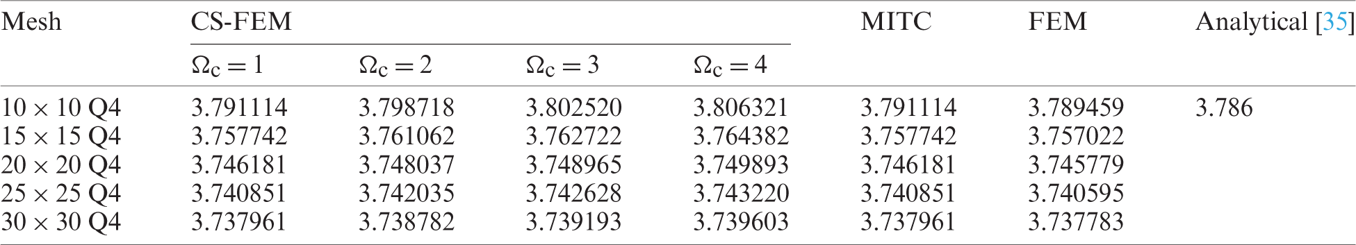
Table 16: Normalized eigenvalues for buckling ( ) considering a SSSS sheet with t/L = 0.2, k = 0.8333 and
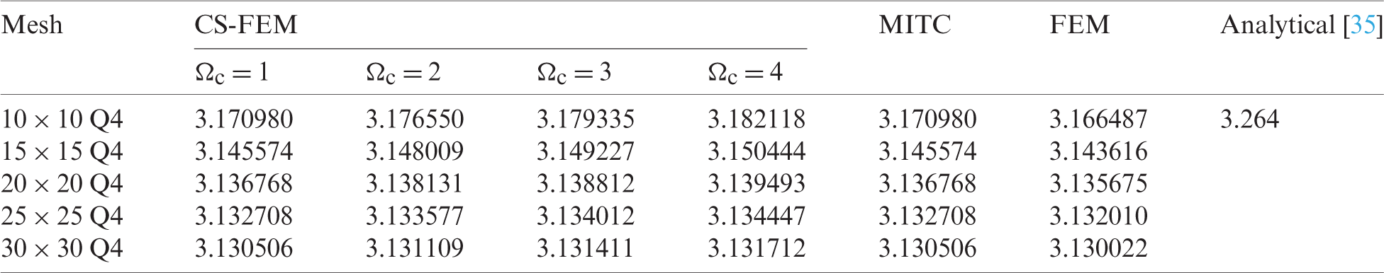
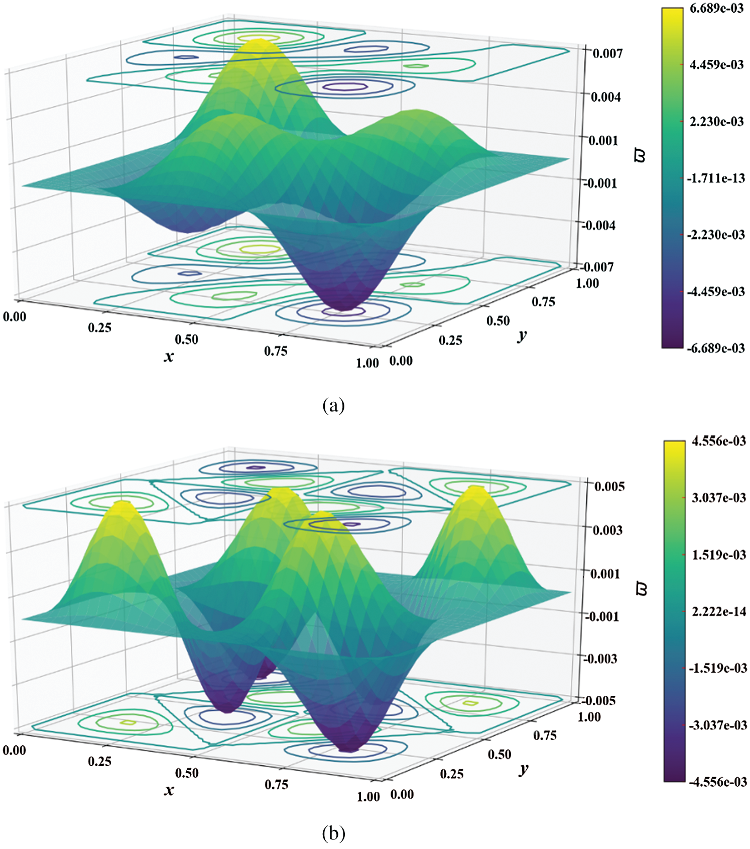
Figure 5: Mode shape of non-dimensional natural frequency  for a CCCC sheet considering t/L = 0.01, k = 0.8601,
  and
and  Q4 mesh for
  for (a) 6th and (b) 12th mode shapes
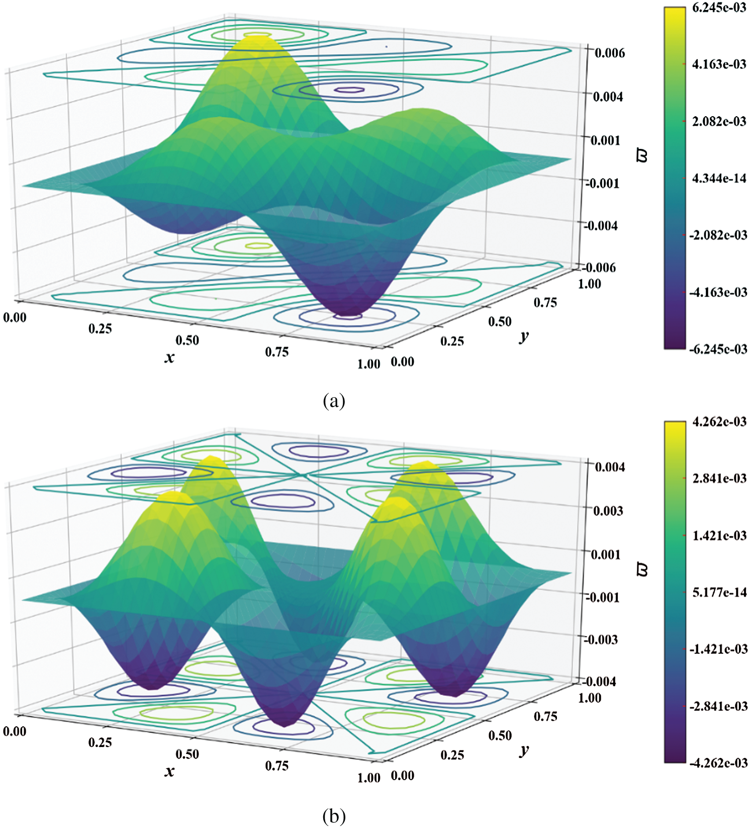
Figure 6: Mode shape of non-dimensional natural frequency  for a SSSS sheet considering t/L = 0.01, k = 0.8333,
  and
and  Q4 mesh for (a) 6th and (b) 12th mode shapes
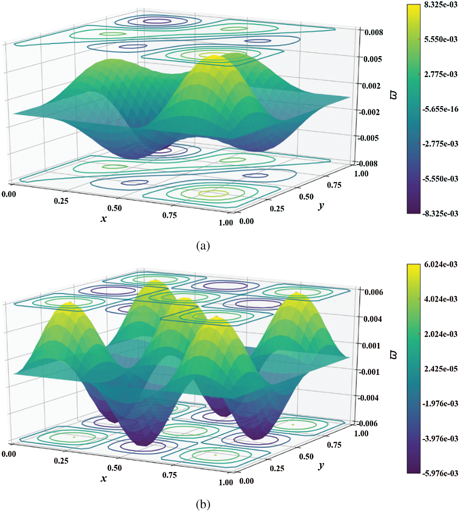
Figure 7: Mode shape of non-dimensional natural frequency  for a CCCC sheet considering t/L = 0.1, k = 0.8601,
  and
and  Q4 mesh for (a) 6th and (b) 12th mode shapes
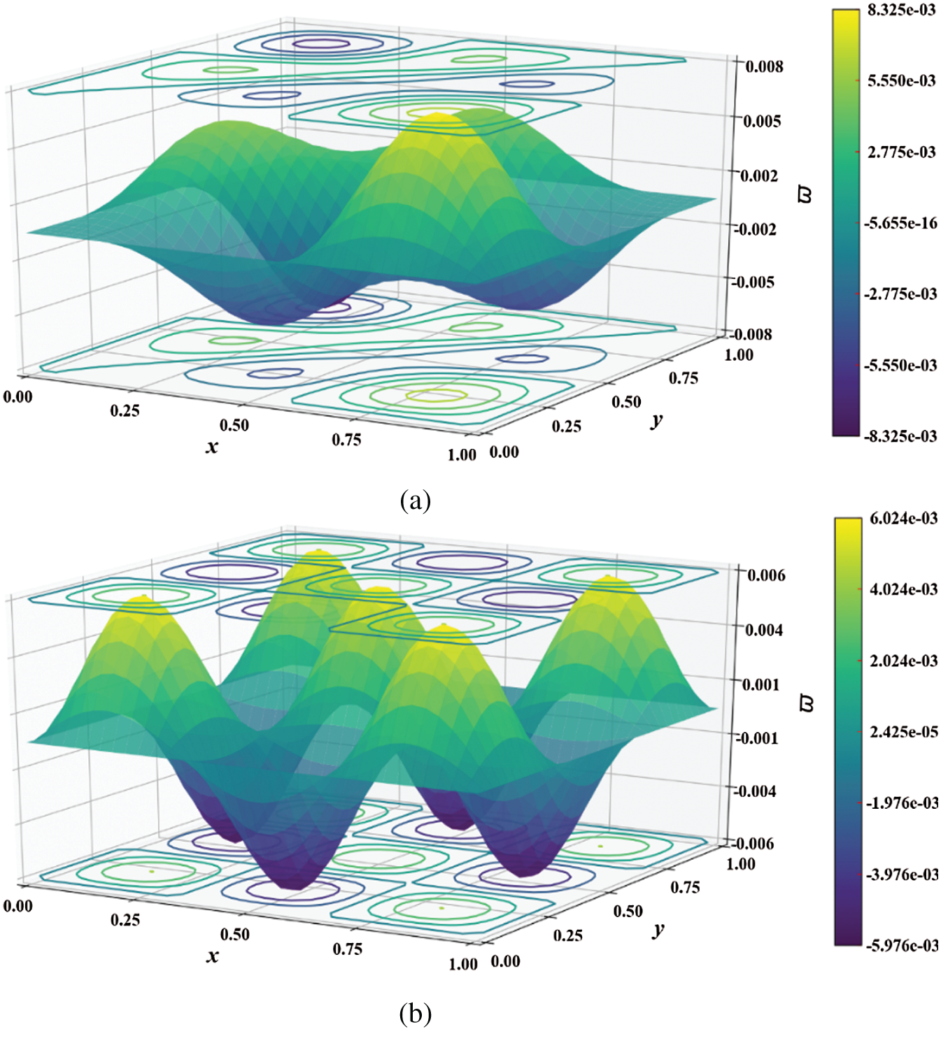
Figure 8: Mode shape of non-dimensional natural frequency  for a SSSS sheet considering t/L = 0.1, k = 0.8333,
  and
and  Q4 mesh for (a) 6th and (b) 12th mode shapes
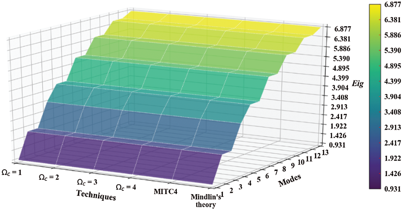
Figure 9: Mode shapes of non-dimensional natural frequency  for a SSSS sheet considering t/L = 0.1, k = 0.8333,
  and
and  mesh
mesh
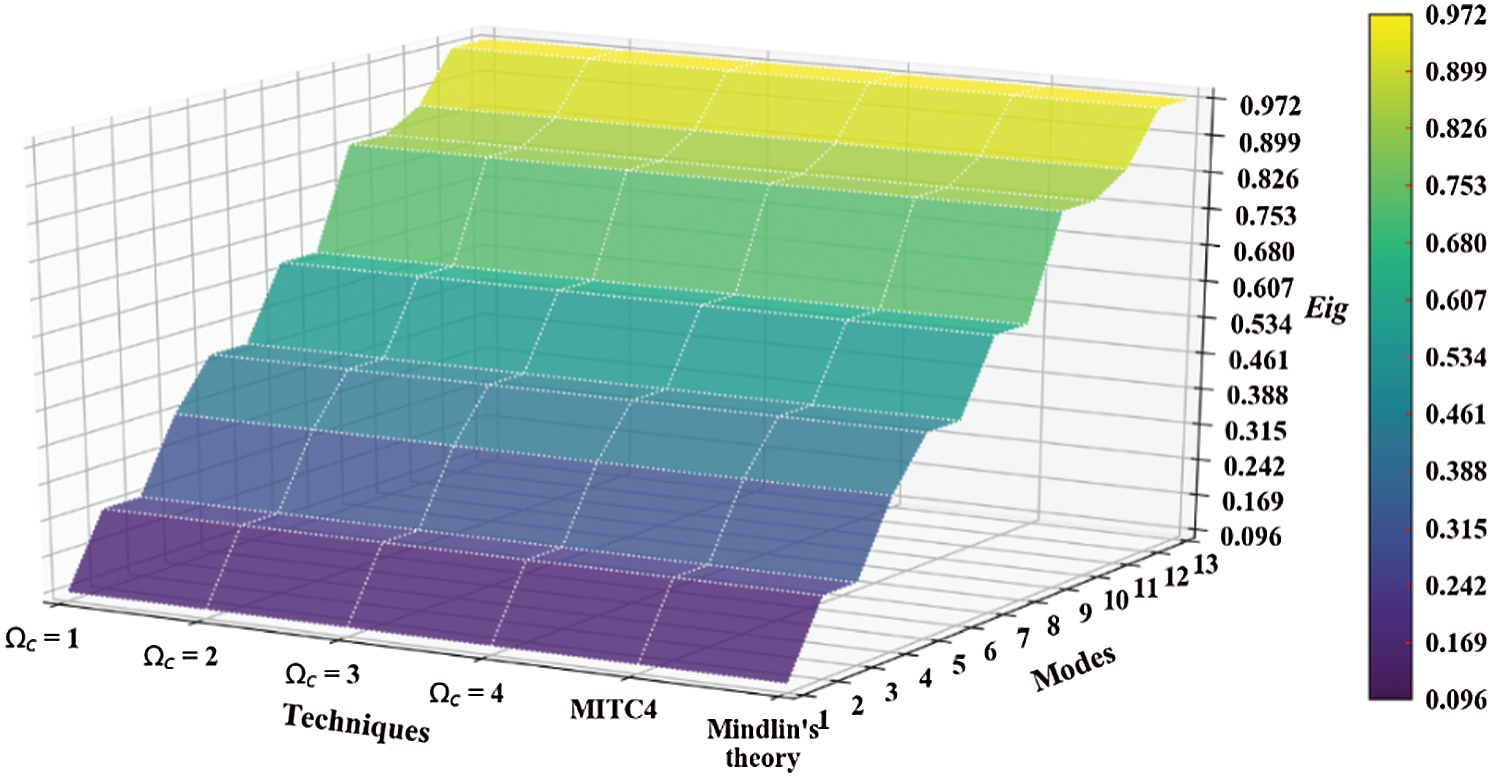
Figure 10: Mode shapes of non-dimensional natural frequency  for a SSSS sheet considering t/L = 0.01, k = 0.8333,
  and
and  mesh
mesh
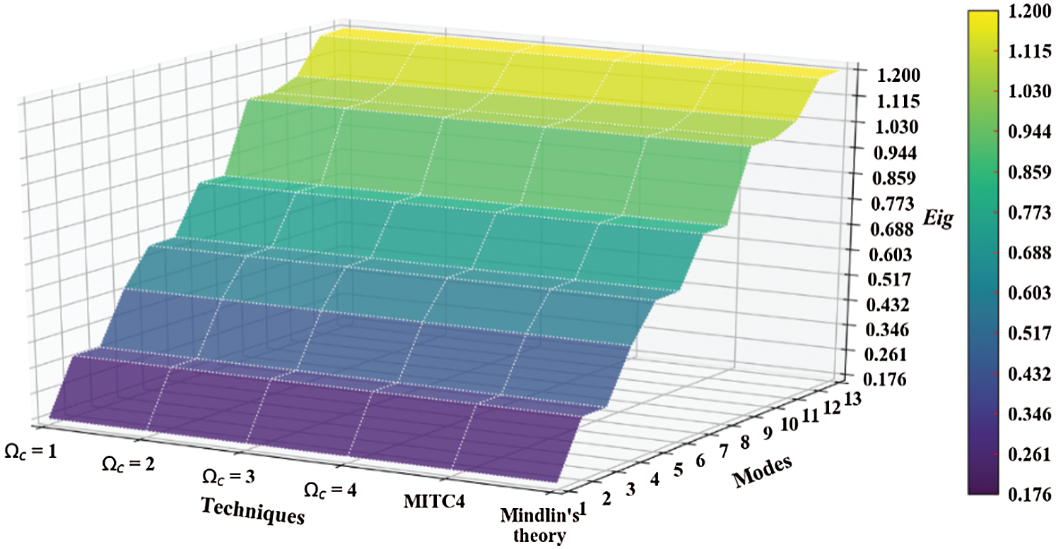
Figure 11: Mode shapes of non-dimensional natural frequency  for a CCCC sheet considering t/L = 0.1, k = 0.8601,
  and
and 

Figure 12: Mode shapes of non-dimensional natural frequency  for a CCCC sheet considering t/L = 0.01, k = 0.8601,
  and
and 
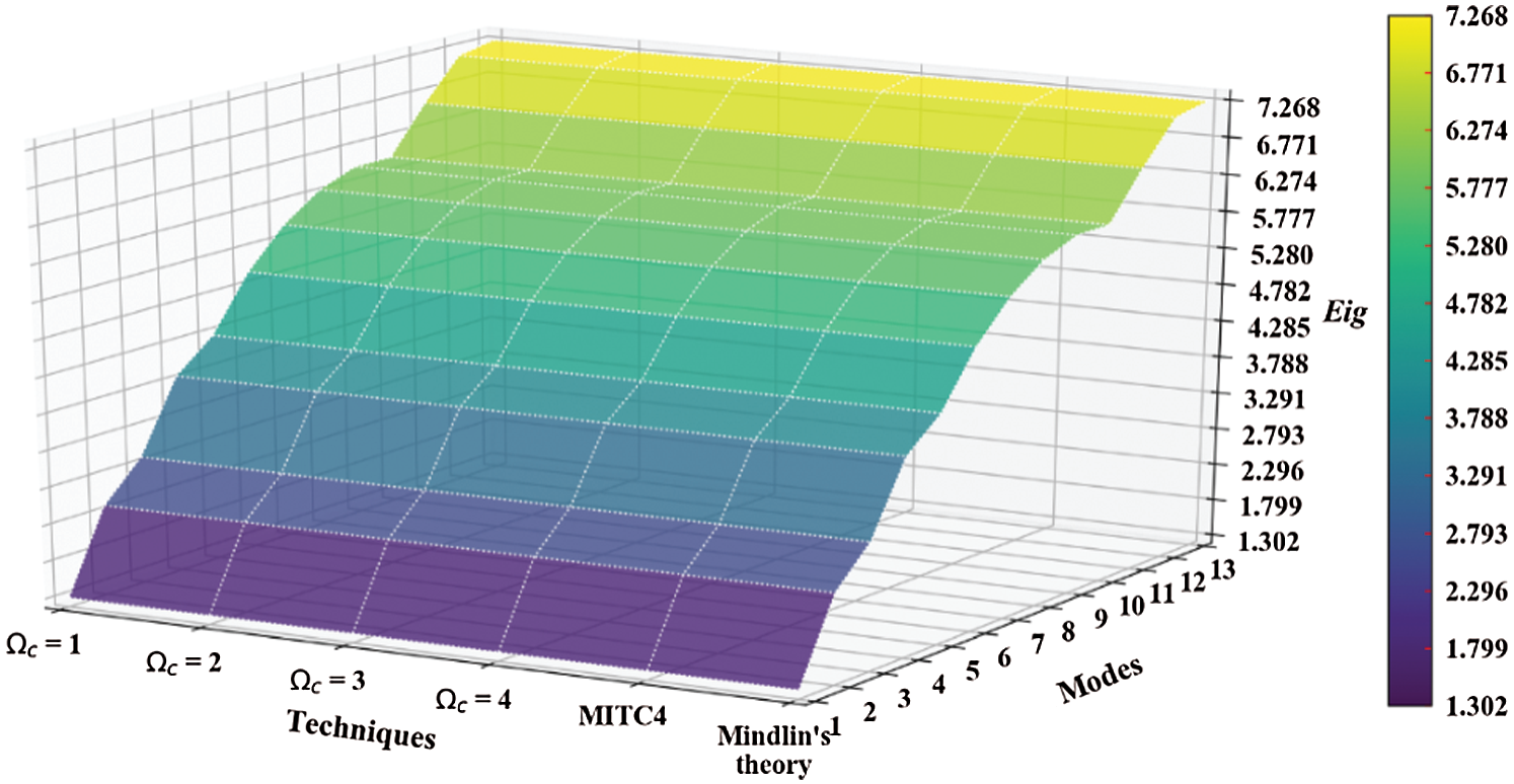
Figure 13: Mode shapes of non-dimensional natural frequency  for a SCSC sheet considering t/L = 0.1, k = 0.8222,
  and
and 
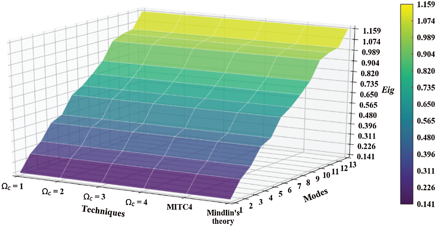
Figure 14: Mode shapes of non-dimensional natural frequency  for a SCSC sheet considering t/L = 0.01, k = 0.8222,
  and
and 
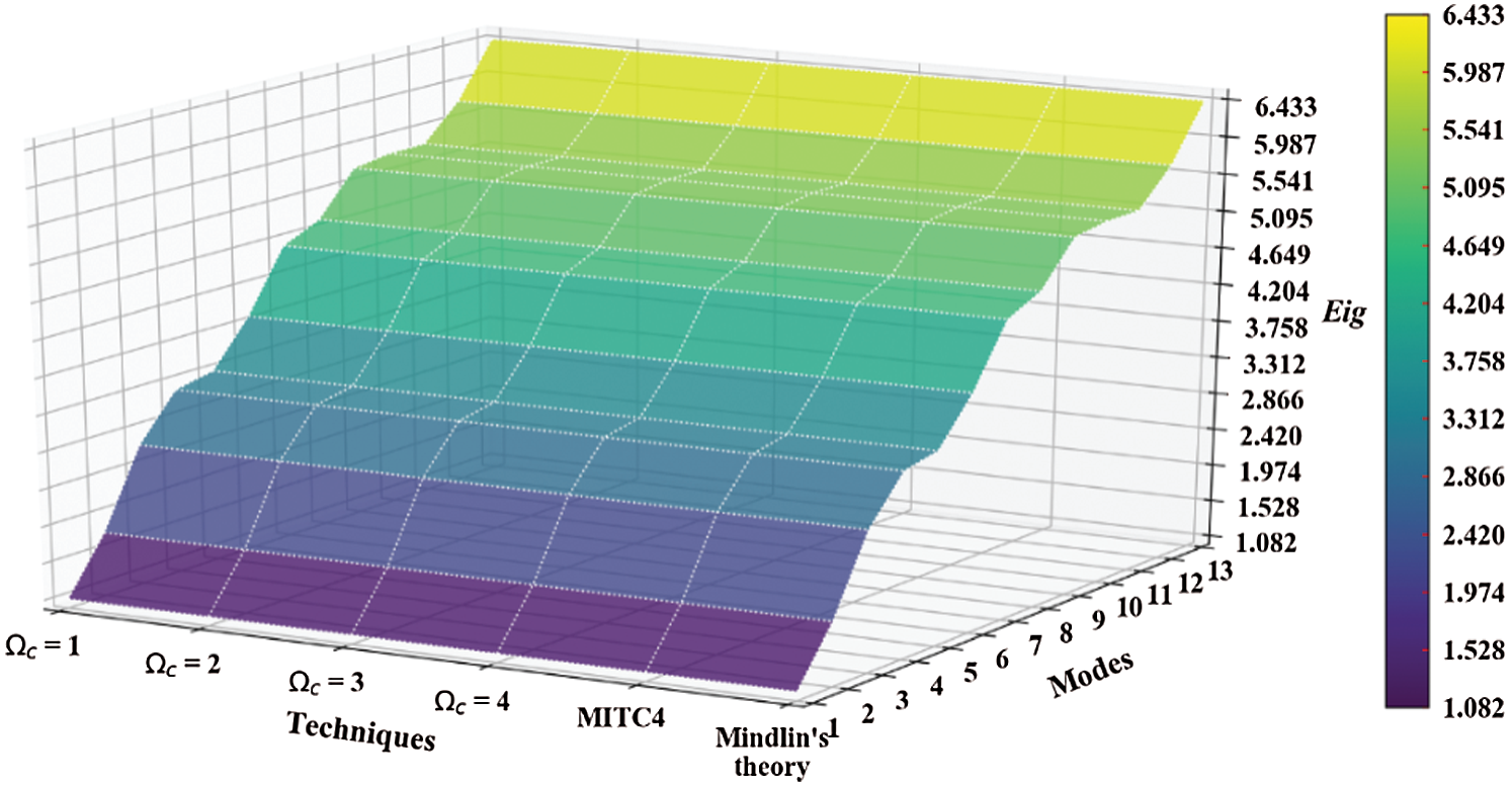
Figure 15: Mode shapes of non-dimensional natural frequency  for a CCCF sheet considering t/L = 0.1, k = 0.8601,
  and
and 

Figure 16: Mode shapes of non-dimensional natural frequency  for a CCCF sheet considering t/L = 0.01, k = 0.8601,
  and
and 
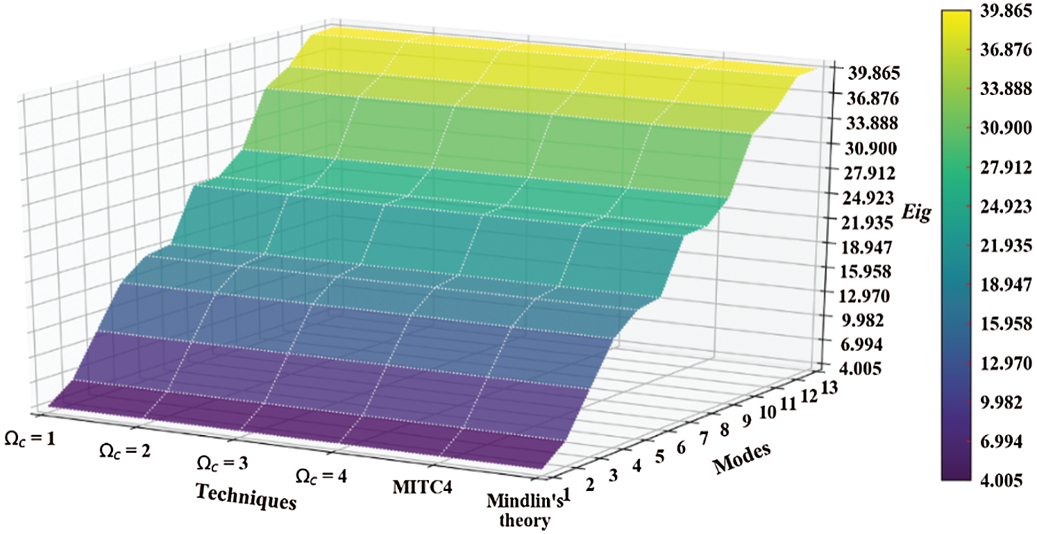
Figure 17: Normalized eigenvalues for buckling ( ) considering a SSSS sheet with t/L = 0.001, k = 0.8333,
  and
and 

Figure 18: Normalized eigenvalues for buckling ( ) considering a SSSS sheet with t/L = 0.05, k = 0.8333,
  and
and 
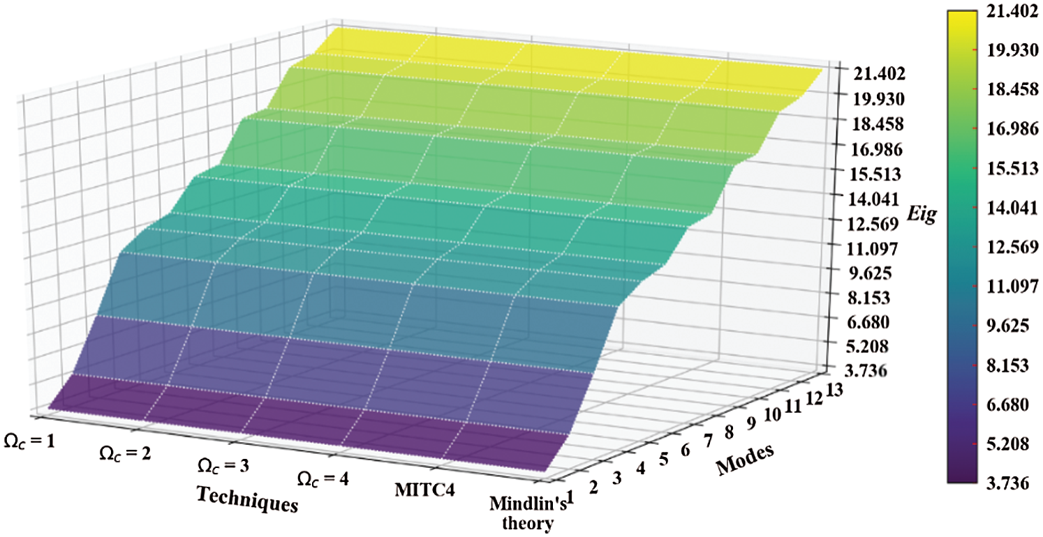
Figure 19: Normalized eigenvalues for buckling ( ) considering a SSSS sheet with t/L = 0.1, k = 0.8333,
  and
and 
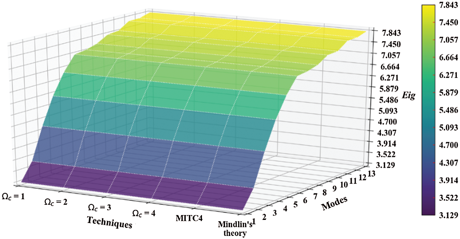
Figure 20: Normalized eigenvalues for buckling ( ) considering a SSSS sheet with t/L = 0.2, k = 0.8333,
  and
and 
A combination of the 4-node quadrilateral mixed interpolation of tensorial components (MITC) element (MITC4) and the cell-based smoothed finite element method (CSFEM) was formulated and implemented to endure free vibration and unidirectional buckling analyses in a rectangular non-woven fabric. A wide range of values for the thickness-to-length ratio were considered, together with edge boundary conditions that are characteristic of many fabric applications. It has been proved that the developed numerical model is able to overcome the shear locking phenomenon with success, revealing both reduced implementation effort and computational cost in comparison to the conventional FEM approach. The numerical results were compared with the ones obtained from a standard finite element computation and analytical solutions for the sake of validation regarding sub-cell integration schemes.
Acknowledgement: The first, third and fourth authors acknowledges FCT for the conceded financial support through Project UID/CTM/00264/2019 of 2C2T—Centro de Ciência e Tecnologia Têxtil, hold by National Founds of FCT/MCTES. The second author is grateful to FCT for the attributed financial funding through the reference project UID/EEA/04436/2013, COMPETE 2020 with the code POCI-01-0145-FEDER-006941.
Funding Statement: This work was supported by the Portuguese Foundation for Science and Technology (FCT) through project UID/CTM/00264/2019 of 2C2T—Centro de Ciência e Tecnologia Têxtil, hold by National Founds of FCT/MCTES, and project UID/EEA/04436/2013, COMPETE 2020 with the code POCI-01-0145-FEDER-006941.
Conflicts of Interest: The authors declare that they have no conflicts of interest to report regarding the present study.
1. P. Roshan. (2019). “Automotive textiles and composites,” in High Performance Technical Textiles, 1st ed. Hoboken, NJ, USA: Wiley, pp. 353–384. [Google Scholar]
2. G. Kellie. (2016). “Developments in nonwoven as geotextiles,” in Advances in Technical Nonwovens, 1st ed. Duxford, UK: Elsevier, pp. 339–364. [Google Scholar]
3. O. C. Zienkiewicz, R. L. Taylor and J. Z. Zhu. (2013). “Background mathematics and linear shell theory,” in The Finite Element Method: Its Basis and Fundamentals, 7th ed. Kidlington, Oxford, UK: Butterworth-Heinemann, pp. 297–392. [Google Scholar]
4. J. K. Knowles and N.-M. Wang. (1960). “On the bending of an elastic plate containing a crack,” Journal of Mathematics and Physics, vol. 39, no. 4, pp. 223–236. [Google Scholar]
5. D. Chapelle and K. J. Bathe. (2011). “Shell mathematical models,” in: The Finite Element Analysis of Shells—Fundamentals, 1st ed. Cambridge, MA, USA: Springer-Verlag, pp. 95–134. [Google Scholar]
6. H. T. Y. Yang, S. Saigal and D. G. Liaw. (1990). “Advances of thin shell finite elements and some applications-version I,” Computers & Structures, vol. 35, no. 4, pp. 481–504. [Google Scholar]
7. T. J. R. Hughes, M. Cohen and M. Haroun. (1978). “Reduced and selective integration techniques in the finite element analysis of plates,” Nuclear Engineering and Design, vol. 46, no. 1, pp. 203–222. [Google Scholar]
8. K. J. Bathe and E. N. Dvorkin. (1986). “A formulation of general shell elements-the use of mixed interpolation of tensorial components,” International Journal for Numerical Methods in Engineering, vol. 22, no. 3, pp. 697–722. [Google Scholar]
9. M. Schwarze and S. Reese. (2009). “A reduced integration solid-shell finite element based on the EAS and the ANS concept-Geometrically linear problems,” International Journal for Numerical Methods in Engineering, vol. 80, no. 10, pp. 1322–1355. [Google Scholar]
10. K.-J. Bathe and E. N. Dvorkin. (1985). “A four-node plate bending element based on Mindlin/Reissner plate theory and a mixed interpolation,” International Journal for Numerical Methods in Engineering, vol. 21, no. 2, pp. 367–383. [Google Scholar]
11. S. Natarajan, A. J. M. Ferreira, S. P. A. Bordas, E. Carrera and M. Cinefra. (2013). “Analysis of composite plates by a unified formulation-cell based smoothed finite element method and field consistent elements,” Composite Structures, vol. 105, no. 1, pp. 75–81. [Google Scholar]
12. R. H. Macneal. (1982). “Derivation of element stiffness matrices by assumed strain distributions,” Nuclear Engineering and Design, vol. 70, no. 1, pp. 3–12. [Google Scholar]
13. E. Carrera, M. Cinefra and P. Nali. (2010). “MITC technique extended to variable kinematic multilayered plate elements,” Composite Structures, vol. 92, no. 8, pp. 1888–1895. [Google Scholar]
14. H. Nguyen-Xuan, S. Bordas and H. Nguyen-Dang. (2007). “Smooth finite element methods: Convergence, accuracy and properties,” International Journal for Numerical Methods in Engineering, vol. 74, no. 2, pp. 175–208. [Google Scholar]
15. M. L. Bucalem and K.-J. Bathe. (1997). “Finite element analysis of shell structures,” Archives of Computational Methods in Engineering, vol. 4, no. 1, pp. 3–61. [Google Scholar]
16. K. C. Park and G. M. Stanley. (1986). “A curved C0 shell element based on assumed natural-coordinate strains,” Journal of Applied Mechanics, vol. 53, no. 2, pp. 278–290. [Google Scholar]
17. M. Cinefra, C. Chinosi and L. D. Croce. (2013). “MITC9 shell elements based on refined theories for the analysis of isotropic cylindrical structures,” Mechanics of Advanced Materials and Structures, vol. 20, no. 2, pp. 91–100. [Google Scholar]
18. K. J. Bathe. (2014). “Finite element nonlinear analysis in solid and structural mechanics,” in Finite Element Procedures, 2nd ed. Watertown, MA, USA: K.J. Bathe, pp. 485–641. [Google Scholar]
19. D. Chapelle and K. J. Bathe. (2011). “Influence of the thickness in the finite element approximation,” in The Finite Element Analysis of Shells—Fundamentals. 1st ed. Cambridge, MA, USA: Springer-Verlag, pp. 259–314. [Google Scholar]
20. E. N. Dvorkin and K.-J. Bathe. (1984). “A continuum mechanics based four-node shell element for general non-linear analysis,” Engineering Computations, vol. 1, no. 1, pp. 77–88. [Google Scholar]
21. P.-S. Lee and K.-J. Bathe. (2005). “Insight into finite element shell discretizations by use of the “basic shell mathematical model,” Computers & Structures, vol. 83, no. 1, pp. 69–90. [Google Scholar]
22. D. Chapelle and K.-J. Bathe. (2000). “The mathematical shell model underlying general shell elements,” International Journal for Numerical Methods in Engineering, vol. 48, no. 2, pp. 289–313. [Google Scholar]
23. H. Nguyen-Xuan, H. V. Nguyen, S. Bordas, T. Rabczuk and M. Duflot. (2012). “A cell-based smoothed finite element method for three dimensional solid structures,” KSCE Journal of Civil Engineering, vol. 16, no. 7, pp. 1230–1242. [Google Scholar]
24. G. R. Liu, T. T. Nguyen, K. Y. Dai and K. Y. Lam. (2007). “Theoretical aspects of the smoothed finite element method (SFEM),” International Journal for Numerical Methods in Engineering, vol. 71, no. 8, pp. 902–930. [Google Scholar]
25. K. Y. Dai and G. R. Liu. (2007). “Free and forced vibration analysis using the smoothed finite element method (SFEM),” Journal of Sound and Vibration, vol. 301, no. 3–5, pp. 803–820.
26. T. J. R. Hughes. (2000). “The C0-approach to plates and beams,” in The Finite Element Method: Linear Static and Dynamic Finite Element Analysis, 1st ed. Mineola, NY, USA: Dover Publications, pp. 310–379.
27. G. R. Liu and T. T. Nguyen. (2010). “Cell-based smoothed FEM,” in Smoothed Finite Element Methods, 1st ed. Broken Sound Parkway, NW, USA: CRC Press, pp. 137–181. [Google Scholar]
28. O. C. Zienkiewicz, R. L. Taylor and J. Z. Zhu. (2013). “Elasticity: Two- and three-dimensional finite elements,” in The Finite Element Method: Its Basis and Fundamentals, 7th ed. Kidlington, Oxford, UK: Butterworth-Heinemann, pp. 211–255. [Google Scholar]
29. N. Gigli and B. X. Han. (2018). “Sobolev spaces on warped products,” Journal of Functional Analysis, vol. 275, no. 8, pp. 2059–2095. [Google Scholar]
30. N. Nguyen-Thanh, T. Rabczuk, H. Nguyen-Xuan and S. P. A. Bordas. (2008). “A smoothed finite element method for shell analysis,” Computer Methods in Applied Mechanics and Engineering, vol. 198, no. 2, pp. 165–177. [Google Scholar]
31. O. C. Zienkiewicz, R. L. Taylor and J. M. Too. (1971). “Reduced integration technique in general analysis of plates and shells,” International Journal for Numerical Methods in Engineering, vol. 3, no. 2, pp. 275–290. [Google Scholar]
32. O. C. Zienkiewicz, R. L. Taylor and J. Z. Zhu. (2013). “The patch test, reduced integration, and nonconforming elements,” in The Finite Element Method: Its Basis and Fundamentals, 7th ed. Kidlington, Oxford, UK: Butterworth-Heinemann, pp. 257–284. [Google Scholar]
33. W. Zeng and G. R. Liu. (2018). “Smoothed finite element methods (S-FEMAn overview and recent developments,” Archives of Computational Methods in Engineering, vol. 25, no. 2, pp. 397–435. [Google Scholar]
34. D. J. Dawe and O. L. Roufaeil. (1980). “Rayleigh-Ritz vibration analysis of Mindlin plates,” Journal of Sound and Vibration, vol. 69, no. 3, pp. 345–359. [Google Scholar]
35. K. M. Liew, J. Wang, T. Y. Ng and M. J. Tan. (2004). “Free vibration and buckling analyses of shear-deformable plates based on FSDT meshfree method,” Journal of Sound and Vibration, vol. 276, no. 3–5, pp. 997–1017. [Google Scholar]
36. A. J. M. Ferreira and N. Fantuzzi. (2020). “Mindlin plates,” in MATLAB Codes for Finite Element Analysis, 2nd ed. Gewerbestrasse, Cham, Switzerland: Springer Nature, pp. 229–267. [Google Scholar]
 | This work is licensed under a Creative Commons Attribution 4.0 International License, which permits unrestricted use, distribution, and reproduction in any medium, provided the original work is properly cited. |