DOI:10.32604/cmc.2021.012422
| Computers, Materials & Continua DOI:10.32604/cmc.2021.012422 | |
| Article |
Multi-Span and Multiple Relevant Time Series Prediction Based on Neighborhood Rough Set
1School of Computer Science and Technology, Nanjing TECH University, Nanjing, 211816, China
2School of Computer Science and Engineering, Kyungpook National University, Daegu, 41566, Korea
*Corresponding Author: Zixu An. Email: anzixu@knu.ac.kr
Received: 30 August 2020; Accepted: 31 December 2020
Abstract: Rough set theory has been widely researched for time series prediction problems such as rainfall runoff. Accurate forecasting of rainfall runoff is a long standing but still mostly significant problem for water resource planning and management, reservoir and river regulation. Most research is focused on constructing the better model for improving prediction accuracy. In this paper, a rainfall runoff forecast model based on the variable-precision fuzzy neighborhood rough set (VPFNRS) is constructed to predict Watershed runoff value. Fuzzy neighborhood rough set define the fuzzy decision of a sample by using the concept of fuzzy neighborhood. The fuzzy neighborhood rough set model with variable-precision can reduce the redundant attributes, and the essential equivalent data can improve the predictive capabilities of model. Meanwhile VFPFNRS can handle the numerical data, while it also deals well with the noise data. In the discussed approach, VPFNRS is used to reduce superfluous attributes of the original data, the compact data are employed for predicting the rainfall runoff. The proposed method is examined utilizing data in the Luo River Basin located in Guangdong, China. The prediction accuracy is compared with that of support vector machines and long short-term memory (LSTM). The experiments show that the method put forward achieves a higher predictive performance.
Keywords: Rainfall and runoff; variable precision fuzzy neighborhood rough set; LSTM; multi-span
Accurate rainfall runoff prediction is of great significance for the protection and management of water resource. As the hydrologic evolution process holds the properties of nonlinearity and uncertainty, exact rainfall runoff prediction is extremely difficult. Currently, much attention for predicting rainfall runoff is still paid to establishing feasible and accurate model. Many machine learning methods have been exploited for time series forecasting, such as artificial neural networks [1–3], genetic algorithm [4], fuzzy theory and support vector machine (SVM) [5]. Despite their successes in this field, there remain several unresolved issues to be addressed before predicting models could move from academic research and become established tools for real-world applications.
Rough set theory, proposed by Pawlak [6–8], is widely used for feature selection, rule extraction and knowledge discovery from categorical data. Rough set describes the uncertainty with the lower and upper approximation, it enhances the discrimination ability on the discrete data. Conventional rough set employs equivalence relations to partition the universe, and generates the mutually exclusive equivalence classes. Granularity relates to the generation accuracy of equivalence classes, and the classical rough set regards the distribution embodied by the individual data as granularity. The granularity is represented by both the individual data and neighboring elements, and the full exploitation of twofold granules [9] would increase the generalization capability of rough set. In the paper these two kinds of granules are utilized for accurately predicting the rainfall runoff.
The preservation of neighborhood structure and order structure is very important for feature extraction and knowledge discovery. For the numerical data processing, such as rainfall runoff prediction, discretization only can deal with individual data, but ignores the internal relationship among data. Neighborhood rough set (NRS) fully considers the neighborhood attributes contained within the data and extends the application scope of rough set. The hydrological rainfall runoff, a special time series data studied in this paper, bears the characteristics of long time span, incomplete and long duration, which bring a high degree of difficulty to the investigation. In the paper, NRS is applied to the rainfall runoff prediction for the first time, which achieves the tradeoff between prediction accuracy and prediction efficiency.
Both feature selection and pattern discovery depend on the scope of data exploitation. Small scope data contains the local feature or pattern, while the large scope data includes its global equivalents. The selection of local or global data depends on the application requirement. The rainfall runoff prediction should follow the double requirements, the forecast should be consistent with the historical data, and it should be accurate in future periods. These two requirements are interrelated. The consistency with historical data enhances the future trend prediction, and accurate future prediction enriches the process of historical data processing. In detail, the rainfall runoff forecast in this paper is to forecast the trend of future multiple periods and use the local data of multiple period to forecast the rainfall runoff.
The contributions of the paper are as follows:
The variable-precision fuzzy neighborhood rough set is firstly applied for rainfall runoff prediction. The variable-precision fuzzy neighborhood rough set is introduced into the rainfall runoff prediction, which makes full use of the neighborhood relationship and trend, while also improving the prediction accuracy.
Multi span times series prediction is proposed in this paper. The rainfall runoff forecast utilizes multi spans data for achieving high prediction accuracy. Compared with the prediction of SVM and long short-term memory (LSTM), the prediction accuracy of the proposed approach achieves a higher degree of accuracy than SVM and LSTM.
The remainder of the paper is organized as follows: in Section 2 the relevant theories are discussed, then a novel rainfall runoff prediction model based on VPFNRS is proposed, next the experimental results and analysis are given, while the last section contains the conclusion and future work proposals.
Rough set theory has been widely used in time series prediction [10–13], such as stock prediction, financial forecasting, hydrological data assimilation, air quality evaluation and so on. Reference [11] developed a novel fuzzy time-series model based on rough set rule induction for forecasting stock indexes. This study employed the rough sets to generate forecasting rules to replace fuzzy logical relationship rules based on the lag period. The experiment shows that the proposed method outperforms the models listed in this paper in error indexes and profits.
Time series forecasting plays an important role in the field of hydrology. Recent trends of time series forecasting are based on data-driven techniques such as Artificial Neural Networks and rough sets. Reference [14] developed a new rainfall-runoff model called SVR-GANN combining SVR with a geomorphologic-based ANN model. The proposed model in simulating the daily runoff was investigated in a case study of three sub-basins located in a semiarid region in Iran. The results are compared with the methods mentioned in the paper. And they show that the proposed model is more accurate. A novel combined model based on the information extracted with ensemble empirical mode decomposition is proposed and validated on three datasets [15]. The model shows better performances with higher prediction accuracy and time efficiency.
The discrete rough set classifier was used to ascertain the threshold of each attribute contributing to landslide occurrence, based upon the knowledge database [16]. Based on Rough Set theory and Petri Net (RSPN), a comprehensive evaluation model for eutrophication of Xiangxi river was established by Yan et al. [17]. The results reveal that the RSPN model can accurately and efficiently analyze the relationship between condition indicators and variations of eutrophication degree.
Rough set theory provides us with another important method of data preprocessing. However, the application of the rough set theory in rainfall runoff forecasting has not been widely studied. In addition, classical rough set theory is based on the equivalence relation, so it is only applied to the data sets with symbolic attributes. However, in practice, many data sets are numerical, so it is necessary to discretize the numerical data. This can lead to the loss of a large amount of information, leading to a decline in knowledge discovery ability. Neighborhood rough set model and fuzzy rough set model are two important methods to resolving this problem. Both models have their own advantages in rough approximation. On this basis, Cheng et al. [11] proposed a fuzzy neighborhood rough set model, which can better process numerical data. This paper presents a rainfall runoff prediction method based on fuzzy neighborhood rough set and introduces a variable precision fuzzy neighborhood rough set model. The method can withstand the influence of noise, thereby reducing the possibility of sample misclassification.
3 Multi-Span and Multiple Rainfall Runoff Prediction
This paper discusses a rainfall runoff prediction method based on the variable-precision fuzzy neighborhood rough set. In order to verify the performance of the models, SVM and LSTM model are introduced for comparison.
3.1 Fuzzy Neighborhood Rough Set
Rough set theory introduced by Pawlak [8] is a new mathematical tool to deal with vagueness and uncertainty in the areas of machine learning, knowledge acquisition, decision analysis, knowledge discovery from big data, expert systems, decision support systems, inductive reasoning, and pattern recognition. Compared with other data mining methods, the major advantage of rough set is that it does not require any additional information. The classical rough set model is just applicable to nominal data. In the real world, the values of attributes may be real-valued. And the real-valued data need to be discretized before the dependency is evaluated. Discretization might lead to information loss and decrease prediction accuracy. In order to solve this problem, neighborhood rough sets and fuzzy rough sets are combined in this paper. Fuzzy theory has been applied in many fields, such as fuzzy reasoning [18], fuzzy control, time series, etcetera.
Definition 1. Let a decision table,  , where U is a nonempty and finite set of sample
  , called a universe, A is a set of conditional attributes
  , and D is a decision attribute.
For  ,
,  , the fuzzy neighborhood relation is defined as follows:

where  is a neighborhood radius with
  ,
,  is an adjustable constant coefficient and
  . Then, if
  , there is a
  .
.
According the Eq. (1), the fuzzy neighborhood of xi is defined as  .
.

Definition 2. Let a decision table,  , where U is a nonempty and finite set of sample
  ,
,  ,
,  . For
. For  , the fuzzy decision of x is defined as follows:

The fuzzy decision  represents the membership degree of x to di induced by B. Then, the fuzzy decision matrix is defined as follows:

Obviously,  holds.
Definition 3. Given two fuzzy sets X and Y on U, the fuzzy inclusion is defined as follows:

where  indicates the sample number which its membership degree to X is less than or equal to Y.
Definition 4. Let a decision table,  , where U is a nonempty and finite set of sample
  ,
,  ,
,  ,
,  is a fuzzy decision matrix.
For  ,
,  is its fuzzy neighborhood induced by B. The variable precision lower approximations
  and upper approximations
  are defined as follows:


Also,


where  represent a row in
  ,
,  and
and  ,
,  . The variable precision positive region is defined as
  .
.
Definition 5. Let a decision table,  , where U is a nonempty and finite set of sample
  ,
,  ,
,  . The variable precision dependency degree of D on B is defined as follows:

It can be deduced that the following expression holds. If  , then
  and
and  .
.
Definition 6. Let a decision table,  , where U is a nonempty and finite set of sample
  ,
,  ,
,  and
and  . The significance
  of a relative to B is defined as follows:

Definition 7. Given a decision table,  ,
,  ,
,  ,
,  . B is named as a reduction of A if it satisfies the following conditions,
  and
and  ,
,  .
.
Definition 8. Let a decision table,  ,
,  ,
,  ,
,  . For ai in A, the fitting fuzzy rule is defined as follows:

where  ,
,  is a combination operation, and
  is a fitting function.
  , D is defined as the fitting coefficients. Then the calculation formula of the fitting fuzzy rule is presented as follows:

Definition 9. Let a decision table,  ,
,  ,
,  ,
,  . For
. For  , the weight of ai is defined as follows:

Apparently,  holds. The weight vector is showed as
  .
.
Definition 10. Let a decision table,  ,
,  ,
,  ,
,  . For
. For  , the fitting fuzzy decision is defined as follows:

Long Short-Term Memory network (LSTM) is a special type of Recurrent Neural Network (RNN). LSTM compensates for the deficiency of RNN in gradient diffusion and explosion. The LSTM also alleviates the insufficient for long short-term memory. The LSTM model replaces the RNN cells in the hidden layer with the LSTM cells, so that they remain in the long-term memory cells. The structure of a standard LSTM is shown as Fig. 1. The LSTM contains three control gates, namely the input gate i, the output gate o and the forgetting gate f.
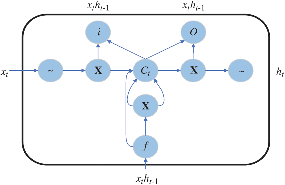
Figure 1: The structure of a standard LSTM unit
In the paper, LSTM is used for the prediction. The first step in LSTM is to determine which information should be discarded from the cell state. This task is accomplished by the forgetting gate layer. The forgetting gate reads the output of the previous cell ht −1, the input of the current cell xt and outputs a value between 0 and 1 for each cell state Ct −1, where “1” stands for complete retention and “0” shows complete abandonment. Eq. (16) describes this process.

where  shows the logistic sigmoid function, ft is the forget gate at time step t and bf represents bias. The following procedure determines how much new information is stored in the current cell state. This step can be described as follows.

where it decides which values to be updated,  represents the candidate values for updating. Then, it and
  are combined to update the old cell state. The new cell state is shown as the following:

Finally, output values are achieved based on the current cell state. The following equations represent this step.

where o t determines which parts of the cell state are exported by running a sigmoid layer. ht is the expected output which is multiplied by o t and a  layer. The cell state is processed by
  to get the value between −1 and 1.
SVM has been introduced as a classification method of solving linear and non-linear problems in [15]. In the real world, most of the problems are nonlinear. The method of solving this limitation is to map the input data into a higher dimensional feature space, and then perform the liner regression in this feature space. The explanatory variables of time series data are the input vectors playing a major role as supports of the training models. For training data  ,
,  ,
,  and
and  . xi is the input vector, yi is the output vector and l is the number of samples. The nonlinear SVM regression (SVR) is defined as the following:

where w is the weighting vector, b is the offset vector and  is the mapping function (also named as the kernel function).
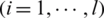
The classification ability of SVM is decided by the training error and classification boundary. SVR achieves the minimization of objective regression function, as Eq. (21) illustration.
where  is the insensitive loss function which controls SVM overfitting degree. If the difference between observed value and predicted one isn’t greater than
  , the predicted value is regarded as non-loss.
  and
and  are the slack variables. C is the penalty coefficient which is used for controlling the influence of the slack coefficient to objective function. SVM optimization function is a convex quadratic, for the sake of simplifying the calculation the dual form is generally adopted, which is defined as Eq. (22).

Subject to  and
and  , where
  and
and  are the Lagrange multipliers,
  is kernel function and L is the number of samples. The nonlinear regression function of SVM is given as Eq. (23), where
  is the number of the support vector.

Non-linear SVM regression need estimate  , C and calculate
  .
.
4 Hydrological Rainfall Runoff Prediction via Fuzzy Neighborhood Rough Set
The main study area (see Fig. 2) is the Luo River Basin located in Guangdong, China, an area of approximately 150 km2. The experimental data come from 4 hydrological control stations along the Nangao reservoir in the Luo River Basin. The original data included daily rainfall, evapotranspiration and runoff observed at four hydrological stations between 1994 and 2003. The original data spanning 10 years were divided into 2 groups. The data from the first 8 years were used as the training sample set, and the data from the latter 2 years were the test sample set. Annual average rainfall is about 2330 mm (during the flood season from April to September, rainfall is about 1890 mm, 81% of the total annual precipitation). The variance of annual precipitation is about 1090 mm2. The average streamflow into the Nangao Reservoir is 8.76 m3/s. Mean annual volume is  . The variance of annual average streamflow is
  .
.
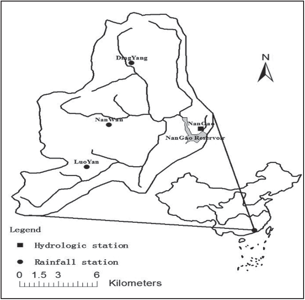
Figure 2: Location map for the study area
The main goal of this paper is to develop a rainfall runoff prediction model for forecasting the streamflow of the Nangao Reservoir. It is well known that the appropriate input variables contain important features about the complex autocorrelation among data set. In general, rainfall(precipitation), previous flows, evaporation, temperature, etc. are associated with the rainfall runoff model. Most studies used rainfall and previous flow as inputs. In this study, the precipitation, previous flows and evaporation are selected as input variables, and the discharge Q serves as the output variable.
In this paper, P is for precipitation and Ep is for potential evapotranspiration. For the convenience of calculation, the value of P is substituted by  in process.
In order to ensure that all variables receive equal weighting during the training process, it is necessary to normalize the raw data (precipitation) to the interval from −1 to 1 or from 0 to 1. Therefore, the presented method processes the scaled data, and the output data are returned to their original scale. The data are normalized between 0.1 and 0.9. The scaling and reverse scaling equations are as follows:


where  is the observed precipitation data,
  is the scaled precipitation data at time t,
  and
and  are the minimum and maximum of the precipitation data series during the simulation period.
  is observed streamflow,
  is normalized observed streamflow,
  is the predicted streamflow using VPFNRS model,
  is the reverse scaled streamflow,
  and
and  are the minimum and maximum of the observed streamflow.
In this study, a VPFNRS model is developed to simulate the streamflow at the Nangao Reservoir. The streamflow responds to the precipitation and runoff from the rainfall-runoff process. The spatial distribution of precipitation is not considered. The average rainfall data were calculated using the Thiesssen polygon method. This data was used as the input data of the VPFNRS model. In the VPFNRS model, we use a concept, N: the time of precipitation impact, which is a parameter in the model. The N represents that the runoff value on the day N is predicted using historical data from the past N days (including rainfall on the previous N days and runoff on the previous N days). Therefore, N is determined as a parameter, which can be selected in the following model structure. The streamflow at time t correlates with the past streamflow at times  . So, the current and the observed times are t −1, t −2, etc. and the future (forecasted) time is t, and the future precipitation (i.e.,
  ) is assumed to be known in this model. Precipitation data that are assumed to be known at times
 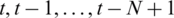 (N day) and streamflow data (simulated) at times
  (N −1 day) are used to predict the streamflow at t (where t denotes the day). The forecasting model applied in real time can be expressed as the following equation:

where the function  indicates the VPFNRS model, t is the time (day),
  and
and  are the normalized precipitation data at times
  (N day).
  are the simulated normalized streamflow at time
 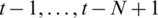 (N −1 day),
  is the simulated normalized streamflow at the future time t.
The work of the presented model includes two stages. Firstly, the variable-precision fuzzy neighborhood rough set theory is used to reduce the input data of the model, so as to simplify the input and improve the efficiency. Secondly, taking the reduction set as the input, the decision rules are extracted based on fuzzy decision making. The reasonable prediction of rainfall runoff is realized. The processing workflow of the VPNFRS prediction model is sketched as pseudocode in Algorithm 1.
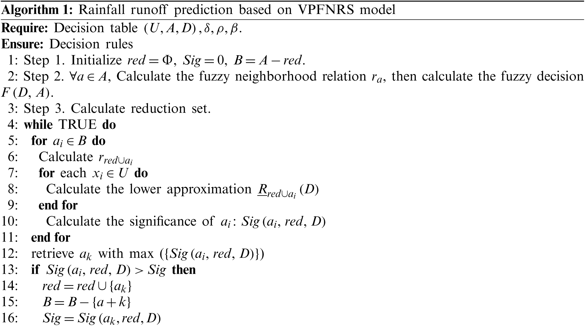
In this section four stages, including data preprocessing, training the proposed model, calibrating model and testing are used for developing a rainfall runoff prediction model based on VPFNRS. The implementation process is shown in Algorithm 1. The code of the VPFNRS model is written in the Python language, and the VPFNRS model is trained on 8 years of data (Year, 1994–2001) for every case. The training data is divided into training set and verification set according to the ratio of 7:3. The original data are normalized according to the formula 22–23 before training the model. Then, all data are discretized to n intervals. Referring to literature [16], the appropriate number of categories for human short memory function is seven, or seven plus or minus two. This study uses 7 as linguistic intervals. The values of each attribute are partitioned into seven linguistic intervals of equal length. The length L could be defined as the following: 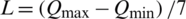 , where
  and
and  are the maximum and minimum of attribute values, respectively. In this way, the predicted results are fuzzy. The fuzzy result is then reduced to the crisp value, which is the midpoint of the corresponding interval. In addition, the root mean square error (RMSE), the correlation coefficient (R), the mean bias error (MBE) and the Nash-Sutcliffe coefficient of efficiency (CE) of the observed and simulated streamflow are used to assess the performance of the rainfall runoff model.
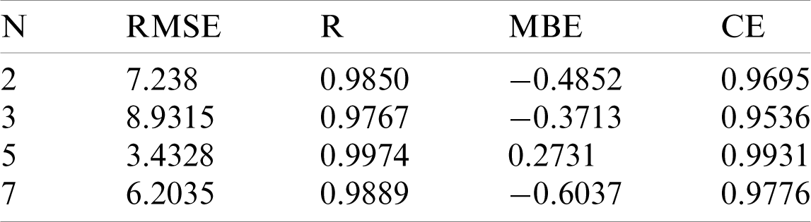
Obtaining the optimal prediction depends on having suitable model parameters. The “N” mentioned above is a parameter that affects the prediction efficiency of the model. In the study, different  were set to train the model to determine the optimal N value. Fig. 3 shows the simulated results during the calibration period and the correlation coefficient using eight years of data for different N. In the case of different N values, better simulated values are obtained during the calibration period. However, the simulation results at N = 5 are better than others. The correlation coefficient R is 0.9974 vs. 0.985 of N = 2, 0.9767 of N = 3 and 0.9889 of N = 7. From Tab. 1, we find RMSE reflects consistent results. The MBE values of the three models in the Tab. 1 show the overestimation or underestimation to different degrees, but the VPFNRS model for N = 5 is still effective. The CE value reflects the confidence of the model. The closer CE is to 1, the higher the credibility of the model. Clearly, the CE value of the VPFNRS model FOR N = 5 days is closest to 1 in Tab. 1 So, we select N to be 5 in the following experiments.
Figure 3: Comparison between observed and simulated daily runoff using different N (N = 2, 3, 5, 7)
Table 1: Statistical characteristics of simulated daily runoff (1994–2001) using different 
To test the performance of the model, this experiment simulates the rainfall-runoff process from DOY (Day of year) 206 (July 25, 2002) to DOY 288 (October 15, 2002) using the VPFNRS model, the SVM model and the LSTM rainfall runoff model. The simulated results of the rainfall-runoff process for the three models are compared, and the advantages and disadvantages of the three models are analyzed. Fig. 4 shows a comparison between the observed and predicted daily runoff by VPFNRS, SVM and LSTM model. The time of precipitation impact (N) is 5 days. We find the forecast results of the three models show great consistency with the actual observed values in the curve trend. During the peak period, it also demonstrates a good fit. However, we can still see the advantage of the VPFNRS model over other models. For example, the observed discharge is 263.3 m3/s in the first peak at DOY 217, the simulated values are 274.57 m3/s for VPFNRS, 336.6 m3/s for LSTM and 228.9 m3/s for SVM. Obviously, the streamflow predicted by VPFNRS model is closer to the observed value. Similar results are shown at several other peak points, such as DOY 230, DOY 231, DOY 260 and so on. The results of statistical analysis in Tab. 2 further confirm this conclusion. For the entire simulation period, the correlation coefficients are 0.9283, 0.8764, 0.9722, and the RMSE are 20.8218, 30.6097, 10.1161 for the LSTM, SVM and VPFNRS model, respectively. From the Tab. 2, we find all three models overestimate the streamflow during the forecast period. And the MBE of the VPFNRS model is minimal. Also, the CE value of the VPFNRS model is closest to 1. All these demonstrate that the proposed model is feasible and reliable.
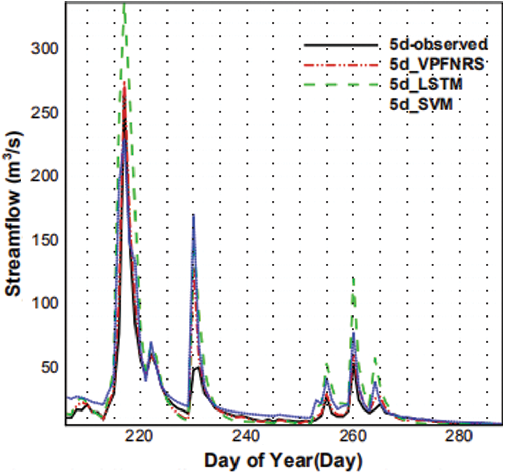
Figure 4: The daily runoff comparison among the observation (DOY 206-288, 2002), the prediction by VPFNRS, SVM and LSTM model for N = 5
Table 2: Statistical characteristics of simulated daily runoff (DOY 206-288, 2002) using three different methods
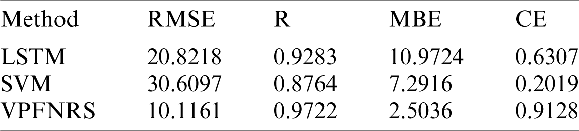
Fig. 5 shows a scatter plot of the simulated streamflow VS the observed streamflow for the SVM, LSTM and the VPFNRS model. The dashed line represents y = x and the dash dot lines indicate y = x −50 and y = x + 50. The forecast period is also DOY 206 to DOY 288 in 2002 year, and N = 5 is still used. Fig. 5 presents that the streamflow is overestimated by the three models. We find that the VPFNRS model performed better than both the LSTM and the SVM models. During the predicting, one scatter plot point for the VPFNRS method fall in the given strip region. Five points fall outside the strip region or on the boundary of the strip region for the LSTM model, and three points fall outside the strip region or on the boundary of the strip region for the SVM model.
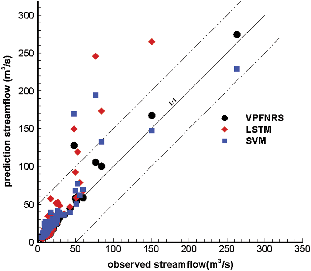
Figure 5: Comparison between observed and simulated daily runoff (DOY 206-288, 2002) using the VPFNRS, SVM and LSTM model for N = 5d
Fig. 6 presents an error comparison of the predicted results using the three models. Clearly the VPFNRS model remains optimal. The figure shows that the absolute error of The VPFNRS model is mostly floating around zero, and the maximum absolute error is about 80, LSTM is about 101, and SVM is about 127. The rainfall on that day (DOY 230) is 99.55 mm2. In addition, in DOY 216, the precipitation is 107.7 mm2, and the absolute error of the three models is respectively 168.9 LSTM, 117.6 SVM and 28 VPFNS model. It was observed that the two days were heavy rainfall days. In other words,the error of the three models is relatively large in the days of heavy rainfall, but the error of the VPFNRS model is still the smallest. The reason for the increased error may be that the underlying surface factor is not considered. Runoff is formed only when precipitation falls on the underside of the basin. The difference of the underlying surface will directly affect the streamflow. Therefore, the underlying surface and climate factors will be considered to improve the prediction efficiency of the model in the later research.
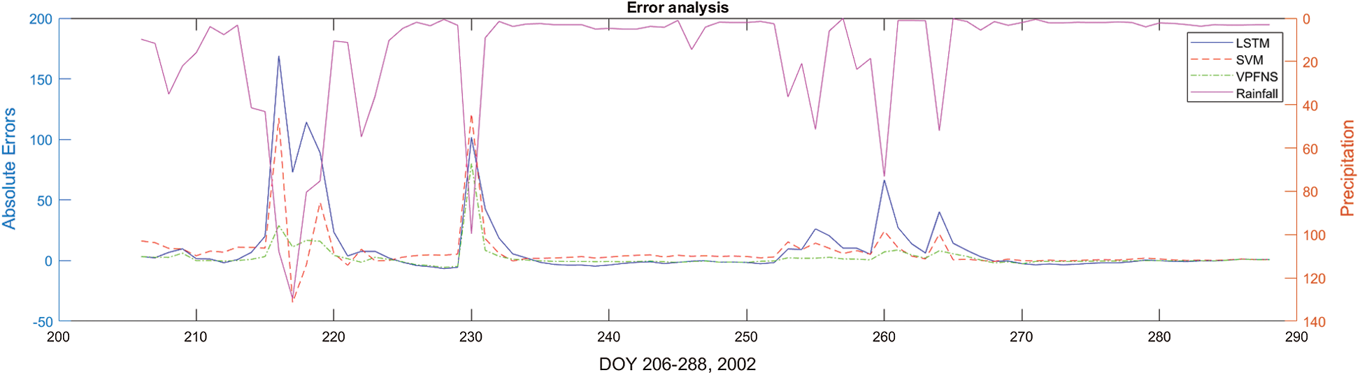
Figure 6: Error comparison of the predicted results using three models
Accurate rainfall runoff prediction is a critical issue in the area of hydrological information processing. In the paper the fuzzy neighborhood rough set is introduced for predicting the rainfall runoff. The proposed method is able to forecast the future rainfall runoff by providing a deep simulation of the essential hydrological factors. The experiments show that the approach presented here could accurately predict the rainfall runoff.
The rainfall and runoff data of different historical length are exploited for predicting the runoff of future variable-length. So the given algorithm has an adjustable predictability, under one framework the same historical data is employed in multiple ways. Meanwhile, the streamflow in different future times can be accurately predicted.
The rainfall runoff prediction method can be extended to similar climactic zones. For different hydrological conditions, it needs to be rectified for predicting the runoff in the new zone. Additionally, the breadth of available historical data for prediction is limited, in the experiment, days beyond 5 would lead to a deterioration in the predictive performance.
Funding Statement: The paper is supported by the National Natural Science Foundation of China (61672279) and the Open Foundation of State Key Laboratory of Hydrology-Water Resources and Hydraulic Engineering, Nanjing Hydraulic Research Institute, China (2016491411).
Conflicts of Interest: The authors declare that they have no conflicts of interest to report regarding the present study.
1. H. Zia, N. Harris, G. Merrett and M. Rivers. (2015). “Predicting discharge using a low complexity machine learning model,” Computers and Electronics in Agriculture, vol. 118, pp. 350– 360. [Google Scholar]
2. C. L. Wu and K. W. Chau. (2011). “Rainfall-runoff modeling using artificial neural network coupled with singular spectrum analysis,” Journal of Hydrology, vol. 399, no. 3–4, pp. 394–409. [Google Scholar]
3. R. Taormina, K. W. Chau and R. Sethi. (2012). “Artificial neural network simulation of hourly groundwater levels in a coastal aquifer system of the Venice lagoon,” Engineering Applications of Artificial Intelligence, vol. 25, no. 8, pp. 1670–1676. [Google Scholar]
4. M. Chlumecky, J. Buchtele and K. Richta. (2017). “Application of random number generators in genetic algorithms to improve rainfall-runoff modelling,” Journal of Hydrology, vol. 553, pp. 350–355. [Google Scholar]
5. X. Li, H. Lu, R. Horton and T. An. (2014). “Real-time flood forecast using the coupling support vector machine and data assimilation method,” Journal of Hydroinformatics, vol. 16, no. 5, pp. 973–988. [Google Scholar]
6. Q. Lei and Z. Xu. (2017). “A unification of intuitionistic fuzzy Calculus theories based on subtraction derivatives and division derivatives,” IEEE Transactions on Fuzzy Systems, vol. 25, no. 5, pp. 1023–1040. [Google Scholar]
7. X. F. Wang, L. Wang, S. J. Li and J. Wang. (2018). “An event-driven plan recognition algorithm based on intuitionistic fuzzy theory,” Journal of Supercomputing, vol. 74, no. 12, pp. 6923–6938. [Google Scholar]
8. Z. Pawlak. (1982). “Rough sets,” International Journal of Computer & Information Sciences, vol. 11, no. 5, pp. 341–356. [Google Scholar]
9. Q. Hu, D. Yu, J. Liu and C. Wu. (2008). “Neighborhood rough set based heterogeneous feature subset selection,” Information Sciences, vol. 178, no. 18, pp. 3577–3594. [Google Scholar]
10. C. Wang, M. Shao, Q. He, Y. Qian and Y. Qi. (2016). “Feature subset selection based on fuzzy neighborhood rough sets,” Knowledge Based System, vol. 111, pp. 173–179. [Google Scholar]
11. C. H. Cheng and J. H. Yang. (2018). “Fuzzy time-series model based on rough set rule induction for forecasting stock price,” Neuro Computing, vol. 302, pp. 33–45. [Google Scholar]
12. R. Taormina and K. W. Chau. (2015). “Data-driven input variable selection for rainfall-runoff modeling using binary-coded particle swarm optimization and extreme learning machines,” Journal of Hydrology, vol. 529, no. 3, pp. 1617–1632. [Google Scholar]
13. N. Ma, J. H. Guan, P. Z. Liu, Z. Q. Zhang and G. M. P. O’Hare. (2019). “GA-BP air quality evaluation method based on fuzzy theory,” Computers, Materials & Continua, vol. 58, no. 1, pp. 215–227. [Google Scholar]
14. M. H. Seiyed and M. Najmeh. (2016). “Integrating support vector regression and a geomorphologic artificial neural network for daily rainfall-runoff modeling,” Applied Soft Computing, vol. 38, pp. 329–345. [Google Scholar]
15. Y. Xiang, L. Gou, L. H. He, S. L. Xia and W. Y. Wang. (2018). “A SVR–ANN combined model based on ensemble EMD for rainfall prediction,” Applied Soft Computing, vol. 73, pp. 874–883. [Google Scholar]
16. S. H. Chang and S. Wan. (2015). “Discrete rough set analysis of two different soil behavior induced landslides in National SheiPa Park Taiwan,” Geoscience Frontiers, vol. 6, no. 6, pp. 807–816. [Google Scholar]
17. H. Y. Yan, Y. Huang and G. Y. Wang. (2016). “Water eutrophication evaluation based on rough set and petrinets: A case study in Xiangxi-River,” Three Gorges Reservoir, Ecological Indicators, vol. 69, pp. 463–472. [Google Scholar]
18. F. Chen, W. H. Xu, C. Z. Bai and X. M. Gao. (2016). “A novel approach to guarantee good robustness of fuzzy reasoning,” Applied Soft Computing, vol. 41, pp. 224–234. [Google Scholar]
 | This work is licensed under a Creative Commons Attribution 4.0 International License, which permits unrestricted use, distribution, and reproduction in any medium, provided the original work is properly cited. |