DOI:10.32604/cmc.2021.015641
| Computers, Materials & Continua DOI:10.32604/cmc.2021.015641 | |
| Article |
Improved Channel Reciprocity for Secure Communication in Next Generation Wireless Systems
1Ind. Reseacher, Neckarstraße 244, PLZ: 70190, Stuttgart, Germany
2Zelle Solutions, Office #FF-37, Saima Square, Gulshan-e-Iqbal, Block-10A, Karachi, Pakistan
3Faculty of Engineering, Bahria University, Lahore Campus, Lahore, Pakistan
*Corresponding Author: Muhammad Khurram Ehsan. Email: mehsan.bulc@bahria.edu.pk
Received: 01 December 2020; Accepted: 24 December 2020
Abstract: To secure the wireless connection between devices with low computational power has been a challenging problem due to heterogeneity in operating devices, device to device communication in Internet of Things (IoTs) and 5G wireless systems. Physical layer key generation (PLKG) tackles this secrecy problem by introducing private keys among two connecting devices through wireless medium. In this paper, relative calibration is used as a method to enhance channel reciprocity which in turn increases the performance of the key generation process. Channel reciprocity based key generation is emerged as better PLKG methodology to obtain secure wireless connection in IoTs and 5G systems. Circulant deconvolution is proposed as a promising technique for relative calibration to ensure channel reciprocity in comparison to existing techniques Total Least Square (TLS) and Structured Total Least Square (STLS). The proposed deconvolution technique replicates the performance of the STLS by exploiting the possibility of higher information reuse and its lesser computational complexity leads to less processing time in comparison to the STLS. The presented idea is validated by observing the relation between signal-to-noise ratio (SNR) and the correlation coefficient of the corresponding channel measurements between communicating parties.
Keywords: Channel measurements; physical layer key generation; channel reciprocity; Internet of things; deconvolution
Next generation of wireless systems specifically 5G, introduces a platform for better exploitation of Internet of Things (IoTs). IoTs do not only require the heterogeneity of the operating devices [1,2], better energy consumption [3] and secure communication are also the major concerns in such wireless systems [4–6]. According to some statistical studies such as [7], there will be more than 30 billion devices wirelessly connected to Internet and also with each other too. This colossal network of devices will evidently require some efficient wireless security measures. One of the promising methods for such wireless security is called Physical Layer Key Generation (PLKG) [8–10]. The Wire-tap channel model is the first method to prove that secrecy can be obtained by exploiting physical layer properties [11]. This method overcomes the discrepancies in initial cryptographic methods such as, exponential operations and computationally bounded security [12]. This approach is then used by the authors in [13,14] to design PLKG technique. One of the key benefits of PLKG is to use information theoretic-security for creating cryptographic keys [15,16]. The principle model of PLKG includes two legitimate nodes Alice and Bob which need to communicate privately and a third node, Eve, who wants to eavesdrop the communication between Alice and Bob. The legitimate nodes send probe signals to each other in order to learn the channel properties. The data in these signals is known beforehand to both nodes and the variation in the data due to channel profile is learned by exchanging such signals. These channel measurements are used to generate a private key. The intrinsic part of this model is to hide these measurements from Eve. The working of PLKG model is based on following fundamental properties i.e., channel reciprocity [17,18], temporal and spatial variation. PLKG assumes a reciprocal channel between Alice and Bob which makes it highly probable that the private key generated at both ends will be similar. The temporal channel variation means that the changes in the channel properties (due to change in ambient temperature, objects in line-of-sight (LOS), noise and interference etc.) can be exploited to ensure the randomness of the private key. This means that each newly generated private key, between Alice and Bob, would be random and different [19]. The spatial variation makes sure Eve should be at safe distance from either of Alice or Bob. If position of Eve is not close to Alice and Bob, it would experience a different channel and the measurements will be different as well. The required distance is estimated by Jake’s model as  /2, where
  is the transmission wavelength. Typically, there is no hard bound for the safe distance and it can vary from case to case [20].
The architecture of PLKG is divided into different blocks which collectively work to produce a private key as shown in Fig. 1, a detailed description about this architecture is provided in [21]. At first, Alice and Bob send pilot signals to each other. These signals are used to acquire channel state information (CSI) or receive signal strength (RSS) of the channel within channel measurement block. Pre-processing block deals with enhancing the reciprocity between Alice and Bob and de-correlating their respective measurement sequences. The processed signal is then passed to quantization block and converted from signal to binary digits, often the resulting binary stream is referred to as pre-key. Afterwards, information reconciliation block is used to reconcile the pre-key among Alice and Bob by using the cascade protocol or the LDPC codes. Privacy amplification block increases the diversity of the reconciled key and it is carried out by using hash functions [22,23]. The focus of this work is on the pre-processing block. Previously, methods like Savitsky Golay filtering along with Walsh, Haar or other similar transform were used for pre-processing [24]. However, these methods lack in certain aspects. The first drawback was the overhead computation required to compensate increased redundancy while enhancing the reciprocity (in the form of de-correlation). Secondly, the recursive nature of reciprocity enhancement, as each measurement has to be processed individually. Thirdly, it fails to address hardware differences such as, front-end attenuation, antenna gain mismatch etc. The incapability of previous reciprocity enhancement model (pre-processing) to cater hardware differences, leads to the further investigation for improving reciprocity. Assuming that the front-end hardware brings imperfection [25], we consider the channel between communicating parties as the effective channel comprising of two parts. First is the true channel which remains same because of being reciprocal. Whereas second is the filter imperfections which vary along the nature of filters.
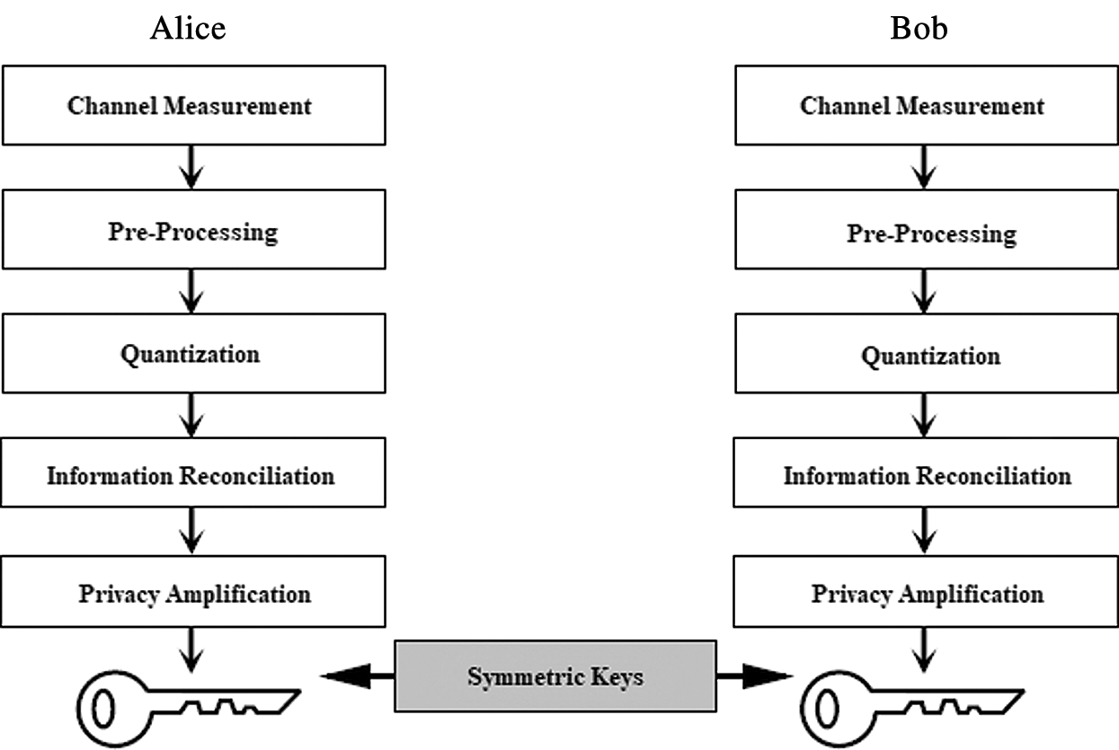
Figure 1: PLKG architecture
According to [26], relative calibration can be used to nullify the effect of filter imperfections. There are several advantages of using relative calibration, e.g., the calibration is executed by signal processing measures and takes place entirely in signal space. Moreover, the relative calibration is easy to be implemented and flexible to be used as it does not require any specific hardware arrangements, especially for dissimilar front-ends of the communicating stations. This is really beneficial when dissimilar front ends are used for the communicating stations.
The researchers have implemented relative calibration in terms of channel coefficients which are obtained in both time and frequency domains. From literature we have discovered that schemes like Channel Gain Compliment (CGC) [27] with focus on frequency response of channel coefficients and exploit the randomness between adjacent frequency sub-carriers at each time instant. The non-reciprocity element in the calibration process is also computed. Furthermore, the hardware differences can be compensated by complementing this non-reciprocity element in each frequency sub-carrier. An extension to CGC is devised in [28] which is referred as a novel transform to mitigate hardware-differences namely, log-domain differential (LDD) transform. The authors claimed that it is a real-time transform which does not require the learning of channel imperfections. In this paper, time domain relative calibration is performed using deconvolution based on Toeplitz and circulant structures.
The contributions of this paper are included as following:
• In order to ensure channel reciprocity, the relative calibration is implemented using state of art deconvolution techniques including the Total Least Square (TLS) and the Structured Total Least Square (STLS).
• Circulant deconvolution technique is proposed as an alternative to the existing techniques and is hypothesized as better performing than the TLS and the STLS.
• The proposed deconvolution technique replicates the performance of the STLS by exploiting the possibility of higher information reuse and its lesser computational complexity leads to less processing time in comparison to the STLS.
• The simulation results of the proposed method also validate that secure communication is possible by adapting the circulant deconvolution within wireless systems having ultra-low latency including 5G and IoTs systems due to its less computational cost.
The paper is organized as follows. Section 2 discusses the system model in hand. Section 3 describes the method of performing the relative calibration. The deconvolution using circulant structure has been introduced in Section 4. Section 5 provides the simulation results. Finally, conclusions are discussed in Section 6. Vectors and matrices are denoted using boldfaced characters. In this paper,  and
and  are the error and the estimated values of x, respectively. The ‘*’ represents the convolution. Parameters indexed by roman characters A and B are associated with the communicating nodes Alice and Bob, respectively.
It is assumed that two nodes A and B referring to Alice and Bob, respectively, need to communicate over a wireless Time Division Duplex (TDD) channel within time duration shorter than channel coherence time. The system model is shown in Fig. 2 which is comprised of cascaded linear filters for both the paths A to B and B to A. The linear filters are consisted of tA, tB, rA and rB as output and input filters respectively, whereas C represents the true channel. The input and output filters are introduced to model as front-end hardware differences [26] which results in the non-reciprocity i.e.,  and
and  . While nA and nB are assumed to be Additive White Gaussian Noise (AWGN) whereas G and H represent the forward and reverse effective channels including the imperfections introduced by the front-end filters, respectively. In the system model, tA, tB, rA and rB are considered time-invariant filters. The reason is that the front-ends vary slower than the channel as discussed in [26]. The forward and reverse chains of the system in Fig. 2 can be expressed as convolution of cascaded linear filters

where G(t,  ) is the forward and H(t,
  ) is the reverse effective channel. The relation between these cascaded chains has been derived in [26] and expressed as

where P( ) is the non-reciprocity element and is modeled as the filter imperfections, which of course is the function of delay only. However, in reality, the filter imperfections are produced by the finite length filters, which can be modeled as
  . If we assume that only one-time instant is considered, then the Eq. (2) can be simplified as

where, g represents vector that contains channel coefficients from forward effective channel, H represents a square matrix of a specific structure covering the channel coefficients of the reverse effective channel and p is a vector that represents the calibration metric. p contains the non-reciprocity part of the channel and that is why it is first learned and then used to rectify erroneous channel measurements as shown in Fig. 3.
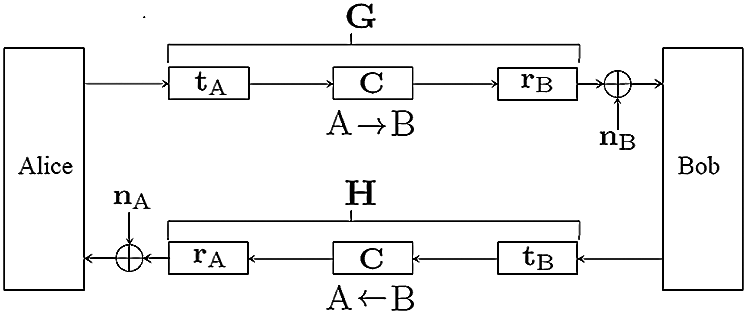
Figure 2: System model
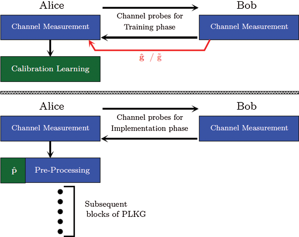
Figure 3: Relative calibration phases. (a) Training phase which uses calibration learning algorithms to obtain  (b) implementation phase which uses
  for compensating the imperfections
3 Relative Calibration through Deconvolution Techniques
To compensate the time-invariant filter imperfection, relative calibration can be performed using the deconvolution techniques. In this section, the deconvolution is performed using the TLS and the STLS as discussed in Subsection 3.1 and Subsection 3.2.
Let us assume that the forward and reverse channel coefficients at kth channel measurement are real, finite-valued and defined as  and
and 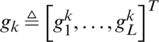 where
where  ,
,  and j
and j 
 . Here L
 , L are the filter lengths and to ensure that the Toeplitz matrix is a square matrix, L
 has to have an odd value. Thus, a relation between L and L
 can be formulated as
  . The calibration vector is defined as
  . The matrix H in (3) is a square matrix of the Toeplitz structure [26]. The kth measurement is represented as
  .
.

It is assumed that  and
and  are affected only by the estimation errors, where the estimated calibration vector p can be obtained using singular value decomposition (SVD) method [29].
For a more realistic approach to address the problem of deconvolution, we assume that both  and
and  are noisy (denoted with a tilde). This modifies the problem given in Eq. (3) as:

Eq. (5) includes  and
and  are the error correction terms for
  and
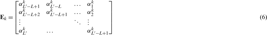
and  respectively. The error correction terms are also structured in the case of STLS which is not the case with TLS and it improves the optimization process. To maintain the symmetry of the equation,
  is transformed into the Toeplitz matrix as well which is denoted as Ek.
As the noise is Gaussian i.i.d (independent and identically distributed), Eq. (5) can be solved by using Maximum Likelihood (ML) method [30]. The Gauss–Newton method [31] is chosen for the ML implementation. In addition, ML optimizes the parameter vector p by minimizing the vector ( +
+ ) in an iterative process. The process of ML is an exhaustive search as it requires much more time than TLS method which is an oversimplified approach. Although STLS is a slower process than TLS, the quality of the p from STLS is far better than TLS, which in turn gives improved calibration. Until now, we have considered a single channel measurement. The assumption can be extended to multiple channel measurements by concatenating successive kth measurements of
  and
and  respectively. A comprehensive equation considering all channel measurements can be given as:
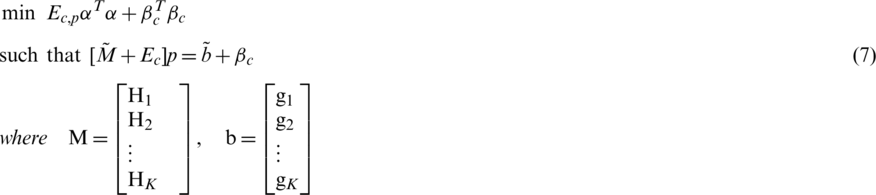
and  denotes the number of training probes. Ec and
  matrices have dimensions [
 ]. Again, Ec is a Toeplitz matrix of
  which is given by
 [26]. Similarly,
 is a single vector that denotes the error correction terms for concatenated
  [26]. Eq. (7) is subjected to the input of the constraint optimization algorithm and an optimized
  is estimated. The matrix or vector with subscript “c” is generated within the algorithm.
Relative calibration is performed in two step fashion as depicted in Fig. 3. The details of which are given as following:
In this phase, Alice and Bob learn the channel imperfections by sending pilot signals to each other. The channel coefficients from Alice to Bob and Bob to Alice are stored  in and
  , respectively, depending upon the coefficients’ nature. Since calibration is performed on Alice side in our case,
  has been sent from Bob to Alice. By doing so, the method of deconvolution can be applied to estimate
  using any of the above-mentioned methods.
In this phase, Eq. (3) is then used to obtain estimated forward channel measurements  by convolving the estimated
  with H.
4 Deconvolution Using Circulant Structure
The limitations of TLS and STLS depend mainly on the structure of H which is Toeplitz, as shown in Eq. (3). However, we can manipulate the performance by using different structure for H. The circulant matrix can be an effective candidate instead Toeplitz matrix. The circulant matrix is defined as a modified Toeplitz matrix which is created by rotating each column or row by one element relative to preceding row or column. In our case, we have rotated a column vector to generate the circulant matrix. The comparison between the circulant matrix and Toeplitz matrix is as following:
4.1 Advantages of Circulant over Toeplitz
In the case of Eq. (3), the number of elements in the matrix H is of great importance. We have to infer the calibration vector p by using channel coefficients from g and H. For calculating more accurate value of p, the number of channel coefficients should be higher in number. Since the circulant matrix is created by using only one vector, a large matrix can be created by using same number of channel coefficients compared to the Toeplitz matrix. Generally, a Toeplitz is defined by two vectors one for row and one for column, the channel coefficient vector h has to split in two further in order to fulfill the condition of being a Toeplitz matrix.
Let us assume we have a vector 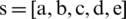 and this has to be transformed into both Toeplitz and circulant matrices.
The vectors results in  and
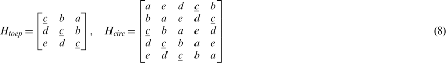
and  matrices as shown in Eq. (8). If every element of this vector is considered as one unit of information then Fig. 4 illustrates how many times an information can be re-used in both types. It clearly shows us that maximum information of circulant is nearly double of what the Toeplitz can achieve (For example displayed in Eq. (8) as the recurring underlined “c”). This gives an edge to circulant over Toeplitz structure. A redundant matrix can increase complexity for circulant structure compared to Toeplitz structure. This happens only if we use SVD for the deconvolution of both, however the results would definitely be better in circulant because of the higher information-reuse. Instead, if Toeplitz structure is used in STLS deconvolution, its complexity also increases because of exhaustive iterations required for MLE execution. Thus, a comparison between the circulant structure using SVD for deconvolution and Toeplitz structure using STLS for deconvolution can be considered fair for the same vector s.
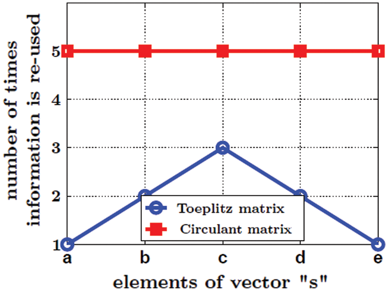
Figure 4: Comparison of the Toeplitz and the circulant matrices’ re-use factor
Recalling Eq. (3) for the deconvolution through circulant, the forward and reverse channel coefficients can now be given as  and
and 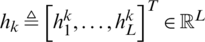 whereas the calibration vector is defined as
 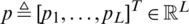 . Note that contrary to Toeplitz, all vectors here are equal in length. This provides the basis for more information re-use. The circulant matrix created by
  would then be:
While using circulant transformation for H in Eq. (3), the calibration vector p can be easily estimated by using SVD and referred as  . This makes it very efficient and less complex to implement. In simple words, circulant deconvolution can be deemed as a scheme that is as efficient as STLS and as simple as TLS. It breaks the trade-off need between STLS and TLS.
The linear model in Fig. 2 is simulated in this section and results are presented for the validation. The simulation environment used here is devised by characterizing the theoretical equations and system model in MATLAB. Fig. 5 shows a prototypical model which is used for simulation purpose. The motivation behind using this is to simplify our original model given the fact that filter imperfections can also be monitored by using single filter per chain.
Figure 5: The simplified model for simulation environment
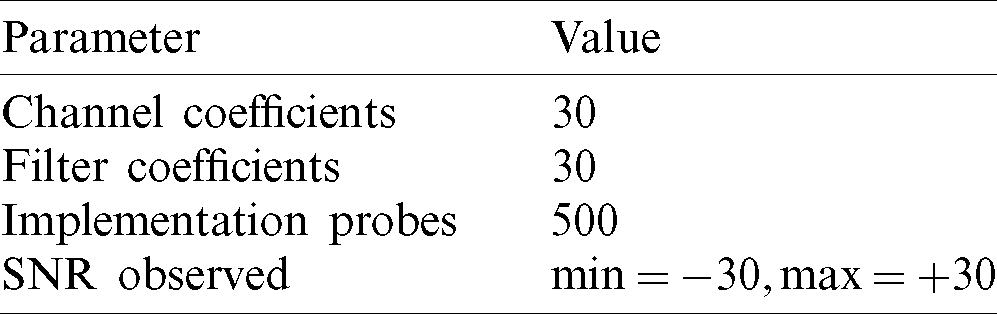
The parameters used for the simulation are shown in Tab. 1. Given the maximum length of the filter is  , where
  0 in the case of Toeplitz (STLS) and
  in the case of circulant.
Table 1: The simulation parameters
In general, the filter responses can be complicated but to keep our assumption simple,  and
and  are modeled as sin(
 ) and sin(
 ) respectively, where
  . The channel C is modeled as Rayleigh distributed fading channel. Contrary to [26], only absolute value of channel coefficients is utilized. The performance of the system is evaluated by comparing the correlation between H and g relative to H and
  . Each simulation has been run for 100 observations and averaged out for a steady response. Fig. 6a shows the SNR versus correlation graph which contrasts the correlation of channel estimates before calibration and after calibration over a wide-range of SNR. Negligible correlation exists in extremely low SNR regions showing the limitation of relative calibration schemes. The reason for this limitation is the noise dominance in the channel coefficient values which does not allow calibration to work properly. However, after a certain SNR, the correlation between channel coefficients of either station becomes visible and it keeps improving from then on. This improvement is visualized in Fig. 6b for STLS and circulant deconvolution schemes. Fig. 6b is a measure of percentage improvement in correlation at any given SNR value.
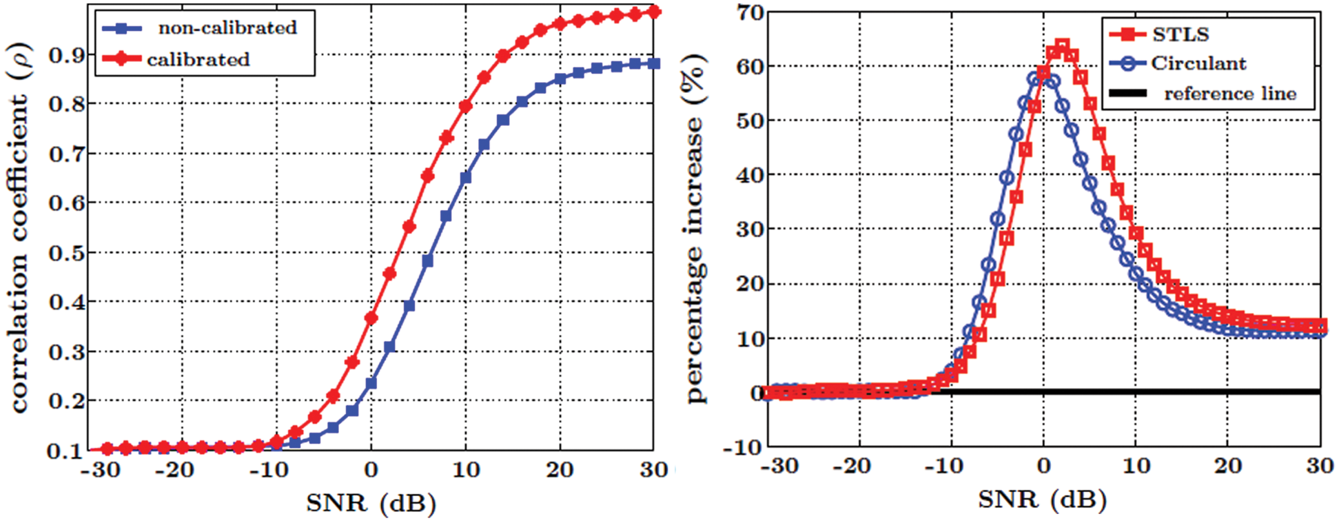
Figure 6: Comparison of STLS and Circulant (a) SNR vs. correlation coefficient graph which shows the effect of calibration on the system (b) shows the percentage improvement in the system performance at different SNR
It can be observed that the circulant performs slightly better in low SNR regions and achieves maximum at 0 dB. The decrease in percentage for both methods in Fig. 6b attributes to the improvement of uncalibrated curve in the positive SNR regions, shown in Fig. 6a. Since there is slight chance for an enhancement, the relative percentage in Fig. 6b decreases and saturates to a single value. The saturation at 10% shows the maximum possible increment which is clearly visible in Fig. 6a. We can observe that the correlation is increasing from 0.88 to 0.98 on 30 dB SNR which translates to 10% increment. Another difference between the two methods is their execution time in terms of the training phase of calibration. The time of training phase is imperceivable to the user or the system in general. Less time it takes to determine the calibration, better would be the system performance. That is why it is an important factor for Physical Security (PHYSEC) systems. Although the execution time of any method greatly depends upon the processing speed of the system and chosen simulation parameters, the comparison between STLS and circulant deconvolution methods is performed by keeping all those factors constant. Fig. 7 depicts such a contrast and is a rather logical comparison then an exact relation between the two methods. As mentioned earlier, an average of 100 observations are taken for each method and their execution times in seconds are recorded by means of MATLAB’s clock command. It is evident that the circulant deconvolution utilizes nearly quarter of the time to provide almost same level of performance as STLS deconvolution, hence it can be regarded as more efficient scheme in terms of relative calibration.

Figure 7: A comparison of average execution time of deconvolution through STLS and Circulant methods
The deployment of relative calibration has introduced as an enhancement in terms of reciprocity in the PLKG architecture which has a major influence in securing communication between nodes. The deconvolution method is proposed in order to implement the relative calibration with less computational cost in comparison to the state-of-the-art methods. Existing deconvolution methods like TLS and STLS are implemented and discussed for comparative purpose. STLS being more efficient than TLS in terms of quality, is used to perform deconvolution however due to its higher computational cost as a trade-off to quality, the circulant deconvolution is proposed as an alternate solution. In this context, a comprehensive comparison between the two methods is also presented, highlighting the reasons and motivation to use circulant deconvolution. It is to be concluded that the circulant deconvolution replicates the performance of STLS even with less computational cost. The simulation results of the proposed method also validate that secure communication is possible by adapting the circulant deconvolution within wireless systems having ultra-low latency including 5G and IoTs systems due to its less computational cost. The proposed circulant deconvolution is recommended as a better scheme in comparison to the state-of-the-art techniques and this is clearly validated by the simulation results. As an immediate succession, the relative calibration is to be implemented over complete PLKG chain and its effect on the created keys should be observed in real time scenarios.
Funding Statement: The authors received no specific funding for this study.
Conflicts of Interest: The authors declare that they have no conflicts of interest to report regarding the present study. Although APC is to be funded by author’s institute under predefined standard policy.
1. M. K. Ehsan. (2020). “Performance analysis of the probabilistic models of ISM data traffic in cognitive radio enabled radio environments,” IEEE Access, vol. 8, pp. 140–150. [Google Scholar]
2. M. K. Ehsan, A. A. Shah, M. R. Amirzada, N. Naz, K. Konstantin et al. (2021). , “Characterization of sparse WLAN data traffic in opportunistic indoor environments as a prior for coexistence scenarios of modern wireless technologies,” Alexandria Engineering Journal, vol. 61, no. 1, pp. 347–355. [Google Scholar]
3. Z. Wuxiong and F. Weidong. (2020). “Energy efficiency in Internet of things: An overview,” Computers Materials & Continua, vol. 63, no. 2, pp. 787–811. [Google Scholar]
4. T. Pecorella, L. Brilli and L. Mucchi. (2016). “The role of physical layer security in IoT: A novel perspective,” Information, vol. 7, no. 3, pp. 49. [Google Scholar]
5. F. S. Ahmad and A. Youseef. (2021). “Packet drop battling mechanism for energy aware detection in wireless networks,” Computers Materials & Continua, vol. 66, no. 2, pp. 45–59. [Google Scholar]
6. J. Xin and L. Mingzhe. (2019). “A Blockchain-based authentication protocol for WLAN mesh security access,” Computers Materials & Continua, vol. 58, no. 1, pp. 2077–2086. [Google Scholar]
7. O. Bay. (2013). “More than 30 billion devices will wirelessly connect to the internet of everything in 2020,” ABI Research. [Online]. Available: https://www.abiresearch.com/press/more-than-30-billion-devices-will-wirelessly-conne/. [Google Scholar]
8. B. Yang and J. Zhang. (2017). “Physical layer secret-key generation scheme for transportation security sensor network,” Sensors, vol. 17, no. 7, pp. 1524. [Google Scholar]
9. G. Li, Z. Zhang, Y. Yu and A. Hu. (2019). “A hybrid information reconciliation method for physical layer key generation,” Entropy, vol. 21, no. 7, pp. 688. [Google Scholar]
10. K. Moara-Nkwe, Q. Shi, G. M. Lee and M. H. Eiza. (2018). “A novel physical layer secure key generation and refreshment scheme for wireless sensor networks,” IEEE Access, vol. 6, pp. 11374–11387. [Google Scholar]
11. A. D. Wyner. (1975). “The wire-tap channel,” Bell System Technical Journal, vol. 54, no. 8, pp. 1355–1387. [Google Scholar]
12. W. Diffie and M. E. Hellman. (1976). “New directions in cryptography,” Information Theory IEEE Transactions, vol. 22, pp. 644–654. [Google Scholar]
13. U. M. Maurer. (1993). “Secret key agreement by public discussion from common information,” Information Theory IEEE Transactions, vol. 39, pp. 733–742. [Google Scholar]
14. C. Ye, S. Mathur, A. Reznik, Y. Shah and W. Trappe. (2010). “Information-theoretically secret key generation for fading wireless channels,” Information Forensics and Security IEEE Transactions, vol. 5, pp. 240–254. [Google Scholar]
15. G. Li, C. Sun, J. Zhang, E. Jorswieck and B. Xiao. (2019). “Physical layer key generation in 5G and beyond wireless communications: Challenges and opportunities,” Entropy, vol. 21, no. 5, pp. 497. [Google Scholar]
16. Y. E. H. Shehadeh and D. Hogrefe. (2015). “A survey on secret key generation mechanisms on the physical layer in wireless networks,” Security and Communication Networks, vol. 8, no. 2, pp. 332–341. [Google Scholar]
17. H. W. Liang, W. H. Chung and S. Y. Kuo. (2018). “FDD-RT: A simple CSI acquisition technique via channel reciprocity for FDD massive MIMO downlink,” IEEE Systems Journal, vol. 12, no. 1, pp. 714–724. [Google Scholar]
18. M. Yuliana and S. Wirawan. (2019). “A simple secret key generation by using a combination of pre-processing method with a multilevel quantization,” Entropy, vol. 21, no. 2, pp. 192. [Google Scholar]
19. L. Cheng, L. Zhou, B. C. Seet, W. Li and D. Ma. (2017). “Efficient physical layer secret key generation and authentication schemes based on wireless channel-phase,” Mobile Information Systems, vol. 2017, no. 12, pp. 1–13. [Google Scholar]
20. Q. Wang, H. Su, K. Ren and K. Kim. (2011). “Fast and scalable secret key generation exploiting channel phase randomness in wireless networks,” in Infocom, Proc., Shanghai, China, IEEE. [Google Scholar]
21. R. Guillaume, F. Winzer and A. Czylwik. (2015). “Bringing phy-based key generation into the field: An evaluation for practical scenarios,” in IEEE 82nd Vehicular Technology Conference, Boston, USA, pp. 1–5. [Google Scholar]
22. J. Carter and M. Wegman. (1979). “Universal classes of hash functions,” Journal of Computer and System Sciences, vol. 18, no. 2, pp. 143–154. [Google Scholar]
23. M. Wegman and J. Carter. (1981). “New hash functions and their use in authentication and set equality,” Journal of Computer and System Sciences, vol. 22, no. 3, pp. 265–279. [Google Scholar]
24. S. Gopinath, R. Guillaume, P. Duplys and A. Czylwik. (2014). “Reciprocity enhancement and decorrelation schemes for phy-based key generation,” in Globecom Workshops, Proc., Austin, TX, USA, IEEE. [Google Scholar]
25. J. Vieira, F. Rusek, O. Edfors, S. Malkowsky and L. Liu. (2017). “Reciprocity calibration for massive MIMO: Proposal, modeling and validation,” IEEE Transactions on Wireless Communications, vol. 16, no. 5, pp. 3042–3056. [Google Scholar]
26. M. Guillaud, D. T. Slock and R. Knopp. (2005). “A practical method for wireless channel reciprocity exploitation through relative calibration,” in Isspa, Proc., Sydney, Australia, IEEE. [Google Scholar]
27. H. Liu, Y. Wang, J. Yang and Y. Chen. (2013). “Fast and practical secret key extraction by exploiting channel response,” in Infocom, Proc., Turin, Italy, IEEE. [Google Scholar]
28. LI. G. and A. Hu. (2015). “A novel transform for secret key generation in time-varying TDD channel under hardware fingerprint deviation,” in IEEE 82nd Vehicular Technology Conf., Boston, USA. [Google Scholar]
29. I. Markovsky and S. V. Huffel. (2007). “Overview of total least squares methods,” Signal Processing, vol. 87, no. 10, pp. 2283–2302. [Google Scholar]
30. N. Mastronardi, P. Lemmerling and S. V. Huffel. (2000). “Fast structured total least squares algorithm for solving the basic deconvolution problem,” Siam Journal on Matrix Analysis and Applications, vol. 22, no. 2, pp. 533–553. [Google Scholar]
31. J. B. Rosen, H. Park and J. Glick. (1996). “Total least norm formulation and solution for structured problems,” Siam Journal on Matrix Analysis and Applications, vol. 17, no. 1, pp. 110–126. [Google Scholar]
 | This work is licensed under a Creative Commons Attribution 4.0 International License, which permits unrestricted use, distribution, and reproduction in any medium, provided the original work is properly cited. |