DOI:10.32604/cmc.2021.015605
| Computers, Materials & Continua DOI:10.32604/cmc.2021.015605 | |
| Article |
An Intelligent Deep Learning Based Xception Model for Hyperspectral Image Analysis and Classification
1Department of Information Technology, University College of Engineering, Nagercoil, 629004, India
2Department of Computer Science and Engineering, University College of Engineering, Ramanathapuram, 623513, India
3Department of Computer Science and Engineering, Kalasalingam Academy of Research and Education, Krishnankoil, 626128, India
4Department of Electrical Engineering, PSN College of Engineering, Tirunelveli, 627152, India
5Department of Entrepreneurship and Logistics, Plekhanov Russian University of Economics, Moscow, 117997, Russia
6Department of Logistics, State University of Management, Moscow, 109542, Russia
7Department of Computer Applications, Alagappa University, Karaikudi, 630001, India
*Corresponding Author: K. Shankar. Email: drkshankar@ieee.org
Received: 30 November 2020; Accepted: 25 December 2020
Abstract: Due to the advancements in remote sensing technologies, the generation of hyperspectral imagery (HSI) gets significantly increased. Accurate classification of HSI becomes a critical process in the domain of hyperspectral data analysis. The massive availability of spectral and spatial details of HSI has offered a great opportunity to efficiently illustrate and recognize ground materials. Presently, deep learning (DL) models particularly, convolutional neural networks (CNNs) become useful for HSI classification owing to the effective feature representation and high performance. In this view, this paper introduces a new DL based Xception model for HSI analysis and classification, called Xcep-HSIC model. Initially, the presented model utilizes a feature relation map learning (FRML) to identify the relationship among the hyperspectral features and explore many features for improved classifier results. Next, the DL based Xception model is applied as a feature extractor to derive a useful set of features from the FRML map. In addition, kernel extreme learning machine (KELM) optimized by quantum-behaved particle swarm optimization (QPSO) is employed as a classification model, to identify the different set of class labels. An extensive set of simulations takes place on two benchmarks HSI dataset, namely Indian Pines and Pavia University dataset. The obtained results ensured the effective performance of the Xcep-HSIC technique over the existing methods by attaining a maximum accuracy of 94.32% and 92.67% on the applied India Pines and Pavia University dataset respectively.
Keywords: Hyperspectral imagery; deep learning; xception; kernel extreme learning map; parameter tuning
Recently, hyperspectral remote sensing images have gained maximum attention among researchers. As the hyperspectral images are robust in solving energy for fine spectra with an extensive range of functions in climatic [1], armed forces, mining, and clinical domains. The application of hyperspectral images is operated on imaging spectrometers, which is implanted in various spaces. The imaging spectrum has been coined in the past decades. It is applied for images in ultraviolet, transparent, closer-infrared, and mid-infrared regions of electromagnetic waves. In imaging spectrometer in massive continuous as well as narrow bands have pixels in the applied wavelength range are completely reflected. Thus, the hyperspectral images are composed of maximum spectral resolution, enormous bands, and dense information. The computational approaches of hyperspectral remote sensing images include image correction, noise limitation, transformation, dimension reduction, and classification.
By considering the benefits of productive spectral data, enormous classical classifiers models like k-nearest-neighbors (k-NN), and Logistic Regression (LR), were deployed. In recent times, efficient feature extraction models and the latest classification have been introduced like spectral-spatial classification as well as local Fisher discriminant analysis (FDA). Recently, Support Vector Machine (SVM) is employed as an efficient and reliable manner for hyper-spectral classifiers, particularly, for tiny training sample sizes. SVM applies ubiquitous 2-class data by understanding the best decision hyper-plane that isolates training instances in the kernel with higher-dimensional feature space. These extensions of SVM in hyperspectral image classifiers are projected for enhancing the classification function. Neural networks (NN), like Multilayer Perceptron (MLP) and Radial Basis Function (RBF), were examined for classifying remote sensing information. In [2], the developers have introduced a semi-supervised NN scheme for large-scale hyperspectral imagery (HSI) classification. Basically, in remote sensing classification, SVM is highly effective when compared with conventional NN with respect to classification accuracy and processing cost. In [3], a deeper structure of NN is assumed as a productive method for classification in which the working function competes with the performance of SVM.
Deep learning (DL) related models have accomplished challenging performance in massive applications. In DL, the Convolutional Neural Networks (CNNs) plays an important role in computing visual-based issues. CNNs are biological-based as well as multilayer classes of DL approach apply NN trained from end to end image pixel values in order to generate the simulation outcome. Using the massive sources of training data and productive execution on GPUs, CNNs has surpassed the traditional models even for human function, on massive vision-based tasks along with image classification, object prediction, scene labeling, house value digit classification, and face analysis. Followed by, the vision tasks in CNN were employed in alternate regions like speech analysis. This is accomplished by predicting the proficient class of methods to learning visual image content, by offering the up-to-date results on visual image classification as well as visual-based issues.
In [4], developers provided a deep neural network (DNN) for HSI classification where Stacked Autoencoders (SAEs) have been applied for extracting differential features. CNN was illustrated for generating optimal classification function when compared with classical SVM classifications and DNNs in visual-based area. Therefore, CNN is applied to visual-based issues which have been deployed for various layers for the HSI classifier. Here, it is evident that CNNs are applied for classifying hyper-spectral data after developing a proper layer structure. Based on these experiments, it is apparent that classical CNNs like LeNet-5 with 2 Conv. layers are not suitable for hyper-spectral data. In [5], feature relations map learning (FRML) is derived to achieve improved HSI classification. The relationships between the features are extracted under the application of a particular function. It uses the CNN model to extract the features and the present pixel is classified into the proper class label. Once the FRML is carried out on the whole image, a precise land usage map is generated.
Though several models are existed in the literature, it is still needed to develop an effective method with improved performance. This paper introduces an effective DL based Xception model for HSI analysis and classification, called the Xcep-HSIC model. Firstly, the Xcep-HSIC model applies a feature FRML for identifying the relationship among the hyperspectral features and discovers many features for enhanced classifier outcome. Subsequently, the DL-based Xception model is applied as a feature extractor to derive a useful set of features from the FRML map. Finally, kernel extreme learning machine (KELM) optimized by quantum-behaved particle swarm optimization (QPSO) is employed as a classification model, to identify the different set of class labels. A series of experiments were carried out using 2 benchmark HSI dataset, namely Indian Pines and Pavia University dataset.
Generally, DL models are composed of massive hidden layers which intend to filter different as well as invariant features of input data. These approaches were operated on the basis of image classification, natural language computation, as well as speech analysis. In recent times, DL technologies have attained massive interest from remote sensing teams. This section explains the review of DL based classification models and ensemble-based classification models for HSI classification.
The brief surveys of the DL approach for computing the remote information are acquired. Chen et al. [6] developed a DL for computing HSI classification. A deep mechanism depends upon the SAE which has been developed for processing feature extraction by achieving the optimal classification accuracy when compared with shallow classifiers. Followed by, Chen et al. [7] present a classification principle named Deep Belief Networks (DBN). The multi-layer DBN approach has been deployed for learning deep features of hyper-spectral data, and learned features are categorized by LR. Ding et al. [8] project the HSI classification approach according to the CNNs, where the convolutional kernels are learned automatically from data using clustering. Wu et al. [9] introduced a convolutional recurrent NN (CRNN) to classified hyper-spectral data. Conv. layers are applied for extracting locally invariant features that are induced into recurrent layers for accomplishing contextual data between diverse spectral bands. Li et al. [10] established a CNN-related pixel-pairs feature extraction approach to HSI classification. The pixel-pair method is developed for exploiting the affinity among the pixels and confirms enough data for CNN. Pan et al. [11] develop a Vertet Component Analysis Network (VCANet) to extracted deep features from HSIs normalized by using a rolling guided filter. Reference [12] presented the different region-relied CNN for HSI classification that encodes semantic context-aware implications for accomplishing challenging features.
2.2 Review of Ensemble Learning Models
The ensemble learning method applies several learning models for accomplishing effective prediction function which is attained from the constituent learning techniques. Ceamanos et al. [13] projected a hyper-spectral classifier according to the combination of various SVM classification models. Huang et al. [14] established the multi-feature classifier which aims in developing SVM ensemble with several spectral as well as spatial characteristics. Gu et al. [15] projected various kernels learning approaches which applies a boosting principle for screening minimum training instances. It makes use of boosting trick for diverse integrations of restricted training instances and adaptively compute the optimal weights of fundamental kernels. Qi et al. [16] imply several kernels learning models that leverage Feature Selection (FS) and PSO.
The workflow contained in the Xcep-HSI method is shown in Fig. 1. As depicted, the Xcep-HSI model performs the FRML map extraction process and then Xception based feature extraction task takes place to derive a set of feature vectors. At last, the QPSO-KELM model is applied to identify the different class labels of HSI.
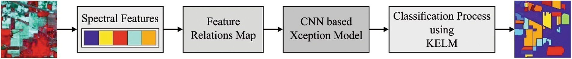
Figure 1: The flow diagram of Xcep-HSI model
3.1 Feature Relations Map Learning
The processes involved in FRML map extraction are given as follows: Initially, the pixels in the image are stored as a high dimensional vector where each element signify the spectral features in every band. Then, the values of every two elements are determined using a normalized difference index (NDI) for constructing a 2-D matrix known as feature relation matrix, subsequently, a matrix is converted into an image for building FRM. This concept is inspired by [5].
In recent times, the DL method is one of the well-known applications evolved from Machine Learning (ML) technology with deepening of multi-layer Feed Forward Neural Networks (FFNN). Under the application of restricted hardware goods, the count of layers in conventional NN is restricted because of learned variables and relations among the layers need maximum calculation time. Using the production of high-end systems, it can be feasible for training deep approaches with the help of multi-level NN.
The DL technique is evolved from CNN with a high rate of function in massive applications like image processing, ML, speech examination, and object prediction. Moreover, CNN is a multi-layer NN [17]. Additionally, CNN is benefited from feature extraction that limits the pre-processing phase to a greater extent. Therefore, it is not sufficient to perform a pre-study for identifying the features of an image. The CNN is collected of Input, Convolutional, Pooling, Fully Connected (FC), Relu, Dropout as well as classification layers. The performances of these layers are defined in the following.
• The input layer is the first layer of CNN. Here, data is provided to this system with no pre-processing. Here, input size differs from pre-trained DL structures are applied. For instance, the input size for the AlexNet method is 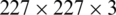 .
.
• Convolution layer has relied on CNN which is applied for extracting the feature maps with the help of pixel matrices of image. Also, it is depending upon the circulation of a specific filter. Consequently, a novel image matrix has been accomplished. Filters have different sizes like  ,
,  ,
,  ,
,  , or
, or  .
.
• The rectified linear units ( ) layer exists behind the Conv. layer. Here, it can be considered as an activation function that follows the negative values that are provided as input to function down to zero. A significant feature that discriminates the function from activation functions like a hyperbolic tangent, sinus has generated robust outcomes. Typically, these functions have been applied for nonlinear conversion operations.
• The pooling layer is computed after Conv. and ReLU mechanism. It is mainly applied for reducing the size of the input and eliminates the system from memorizing. As the Conv. layer, the pooling procedure applies diverse sized filters. This filter considers max or average pooling functions on image matrices which considers the particular attribute. Followed by, maximum pooling is applied as it showcased optimal function.
• FC layer emerges after Conv, ReLU as well as Pooling layers. The neurons in this layer are attached to the regions of the existing layer.
• A dropout layer is applied for eliminating the network memorizes. A performance of this approach is computed by the arbitrary elimination of few nodes of a system.
• The classification layer is evolved after FC Layer where the classification process has been performed. In classification, probability values refer to that it is nearby the class. These measures are accomplished with the help of the softmax function.
Xception model
In this study, DL based Xception architecture is utilized to extract the features. The Xception system is identical to inception (GoogLeNet), whereby the inception is replaced by depth-wise separate Conv. layers. In particular, Xception’s structure is developed according to the linear stack of a depth-wise separate Conv. layer (36 conv. layers) with a linear residual attached (Fig. 2) [18]. In this model, there are 2 significant Conv. layers are used namely, depthwise and pointwise conv. layer. In depth-wise conv. layer, a spatial convolution takes place automatically in channels of input data, and point-wise conv. layer, in which a  conv. layer maps the result of novel channel space under the application of a depth-wise convolution.
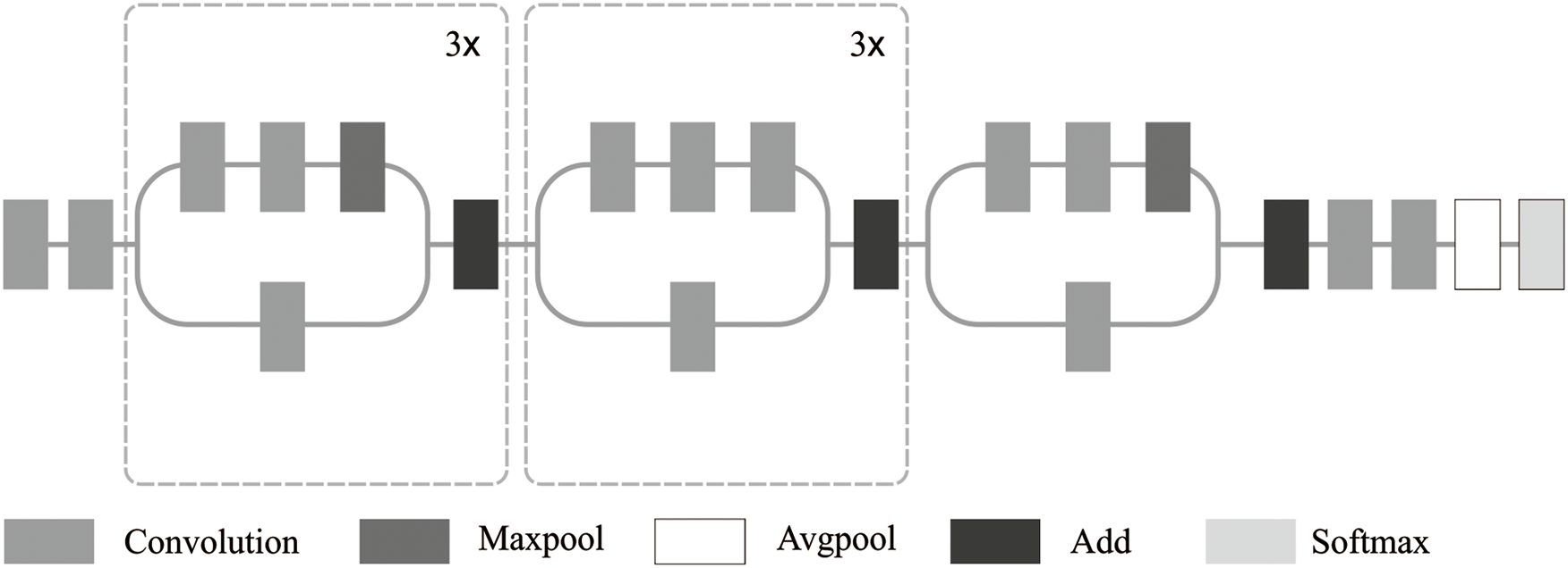
Figure 2: The structure of the xception model
3.3 QPSO-KELM Based Classification
ELM is defined as a novel learning approach for training “generalized” single hidden layer feedforward neural networks (SLFNs) that are applicable to gain supreme generalization function with robust learning speed on complex issues. ELM contains input, hidden as well as output layer, in which input and hidden layers are linked using input weights whereas output and hidden layers are linked using resultant weights. In contrast with CNN, ELM does not require regular parameter modification. The base ELM is classified into 2 major phases namely, ELM feature mapping as well as ELM parameter solving [19]. Initially, a concealed depiction is attained from actual input data through nonlinear feature mapping. Based on the ELM principle, diverse activation functions could be applied in the ELM feature mapping phase. Secondly, output weight parameters are resolved using MoorePenrose (MP) generalized converse and lower norm least-squares solution of a typical linear method with no learning rounds. It is applied that N various training samples have been employed,  , in which
  signifies a d-dimensional input vector as well as
  denotes a c-dimensional target vector. The ELM system along with Q hidden nodes are depicted as given below:

where  implies the input weight vector, bj refers to the hidden layer bias, and
  indicates the final weight vector for jth hidden node.
  represents the final value of jth hidden node. In the case of simplification, Eq. (1) is illustrated as

where H denotes the hidden layer outcome matrix and  implies the resultant weight matrix.
As ELM has massive benefits, massive ELM variants have been presented for reporting the functions of remote sensing. Next, the better function of ELM on HSIs are applied in real-time applications. Kernel learning models are evolved from ML approaches for identifying the typical relationships among features and labels. When compared with common applications, kernel learning approaches perform optimally in accelerating the nonlinear associations from features and labels. Usually, nonlinear connections from pixels and ground covers exist in HSIs. In order to resolve these problems, the KELM framework is projected as a classifier in spectral-spatial classification approach. Also, it unifies kernel learning with ELM and expands the explicit activation function into an implicit mapping function that eliminates arbitrarily produced attribute problems and showcases the supreme generalization ability. Followed by, KELM is applied extensively as a classification approach for predicting the ground covers for every pixel. Fig. 3 illustrates the network structure of the KELM model.
Figure 3: The network structure of KELM
The combination of actual spectral features Xspec and learned spatial features Xspat, and spectral-spatial features  are obtained. In order to equate the function (2), the final weight matrix is determined as,

where H+ implies the MP generalized converse for H. Basically, matrix H+ is illustrated as H+ = HT(HHT)−1, in which HT denotes transpose of H. In order to get generalization, true value C is included with diagonal units of HHT. Hence, Eq. (3) is depicted as 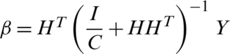 , which attains the least-squares estimation cost function for resolving
  . The applied input spectral-spatial data
  , the ELM classification models is equated mathematically as shown below:

In ELM, feature mapping  are unknown to the user. Hence, Mercer’s condition has been applied as a kernel matrix for ELM in the form of,

where the ith row as well as rth column units are  . In the case of ith row vector in
  . Therefore, the summarization of KELM is implied as,
To enhance the function of the newly presented spectral-spatial classification model, the QPSO algorithm has been applied for computing the parameter C for KELM.
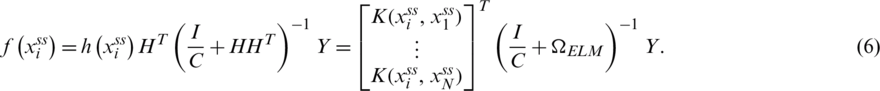
In Liu et al. [20] presented a QPSO that eliminates the velocity vector of actual PSO and prominently modifies the upgrading principle of particles’ location for searching effective element. Initially, QPSO is a combination of quantum computing as well as PSO. Then, QPSO depends upon the implication of the quantum state vector. It uses the probabilistic amplitude depiction of quantum for coding the particles that creates a particle with the superposition of massive states and employs quantum rotation gates for realizing the upgrade the performance. Fig. 4 shows the flowchart of QPSO model [21]. The iterative function of QPSO is varied from PSO. Followed be, in contrary PSO, QPSO requires no velocity vectors for particles and some parameters for modifying and make the implementation simpler. The upgraded principle of particles’ location of QPSO is defined in the following:

where N implies the population of particles; D denotes the dimension of issues;  refers the location of particle;
  defines the local best position;
  signifies the global best position;
  represents mean local best positions.
Figure 4: The flowchart of QPSO algorithm
The performance of the Xcep-HSIC model is simulated using Intel i5, 8th generation PC with 16 GB RAM, MSI L370 Apro, Nividia 1050 Ti4 GB. For simulation, Python 3.6.5 tool is used along with pandas, sklearn, Keras, Matplotlib, TensorFlow, opencv, Pillow, seaborn and pycm. The experiments are conducted on 2 benchmark HSI datasets [22] such as Indian Pines and Pavia University dataset. For experimentation, 50% of data is used for training and testing correspondingly. The parameter setting of PSO algorithm is, population size: 20, maximum particle velocity: 4, initial inertia weight: 0.9, final inertia weight: 0.2, and maximum number of iterations: 50. The parameters involved in ELM are filter count: 17, pooling window size: 17 * 17, number of convolution branches: 2, and convolution filter size: 15 * 15. Finally, the parameter setting of CNN model are listed here, batch size: 50, epoch count: 10, learning rate: 0.05, and momentum: 0.9. A detail related to the dataset and the obtained outcomes is discussed in the subsequent sections.
The Indian Pines dataset is illustrated in Fig. 5. It is composed of  pixels and 224 spectral reflectance bands from the wavelength range 0.4–2.5
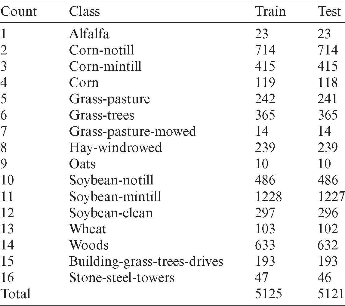
  m. This view is comprised of maximum agriculture and a minimum of forests or alternate natural perennial vegetation. Here, 2-lane highways, one rail line, and few low-density housing, alternate building formations as well as smaller roads. Because of newly developed crops in June, corn and soybeans are in the primary stage of development with coverage by 5%. An accessible sample is classified as 16 classes for a sum of 10,366 samples as depicted in Tab. 1. The count of bands is limited by 200 while eliminating the band covering the water absorption region.
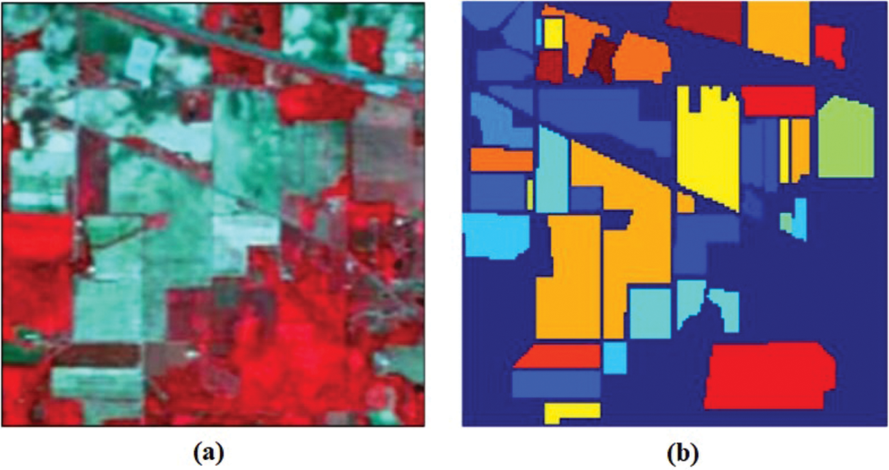
Figure 5: Indian Pines dataset (a) sample image (b) ground truth
The Pavia University dataset is illustrated in Fig. 6. It is composed of  pixels and 103 spectral bands along with a spatial resolution of 1.3 m, however, few samples in an image are not embedded with details and should be removed before examination. The actual category is classified as 9 with a total of 42,761 samples as depicted in Tab. 2.
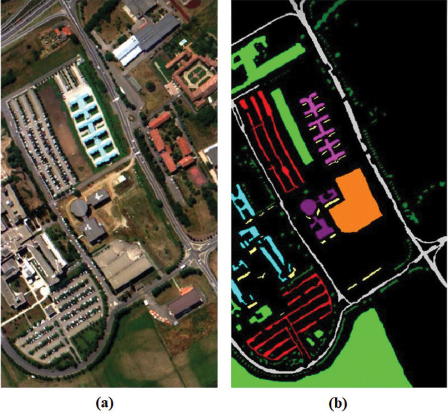
Figure 6: Pavia University dataset (a) sample image (b) ground truth
Table 2: Pavia University dataset
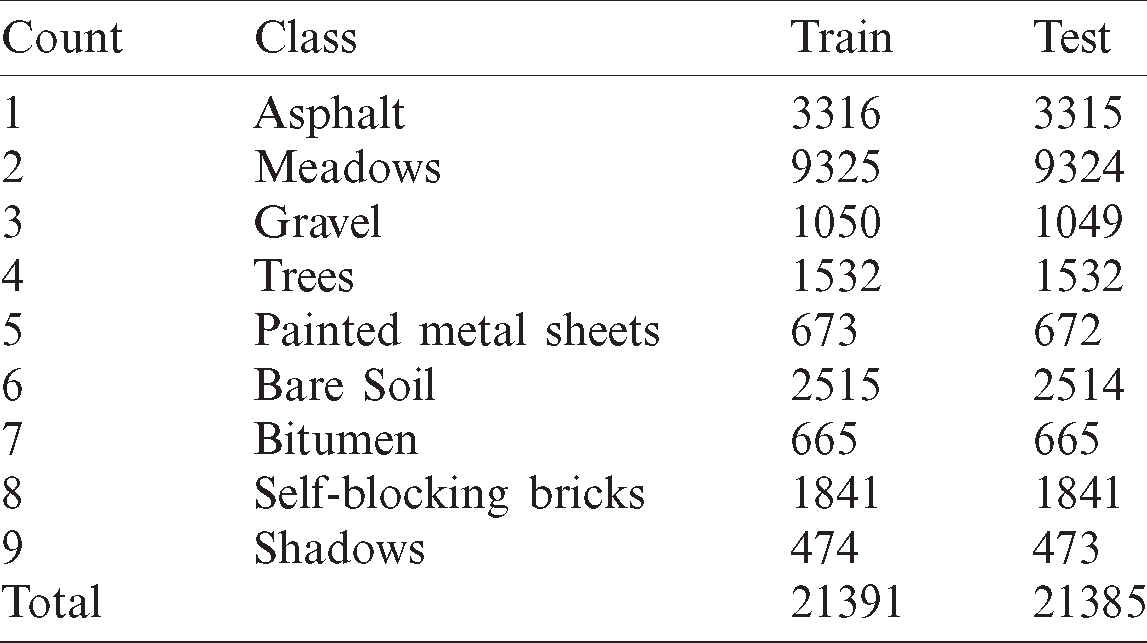
Fig. 7 visualizes the accuracy and loss graphs attained by the presented model on the India Pines and Pavia University dataset. Fig. 7a shows the accuracy graph of the Xcep-HSIC model on the applied India Pines dataset under a distinct number of epochs. The figure portrayed that the training and validation accuracies get increased with an increase in the number of epochs.
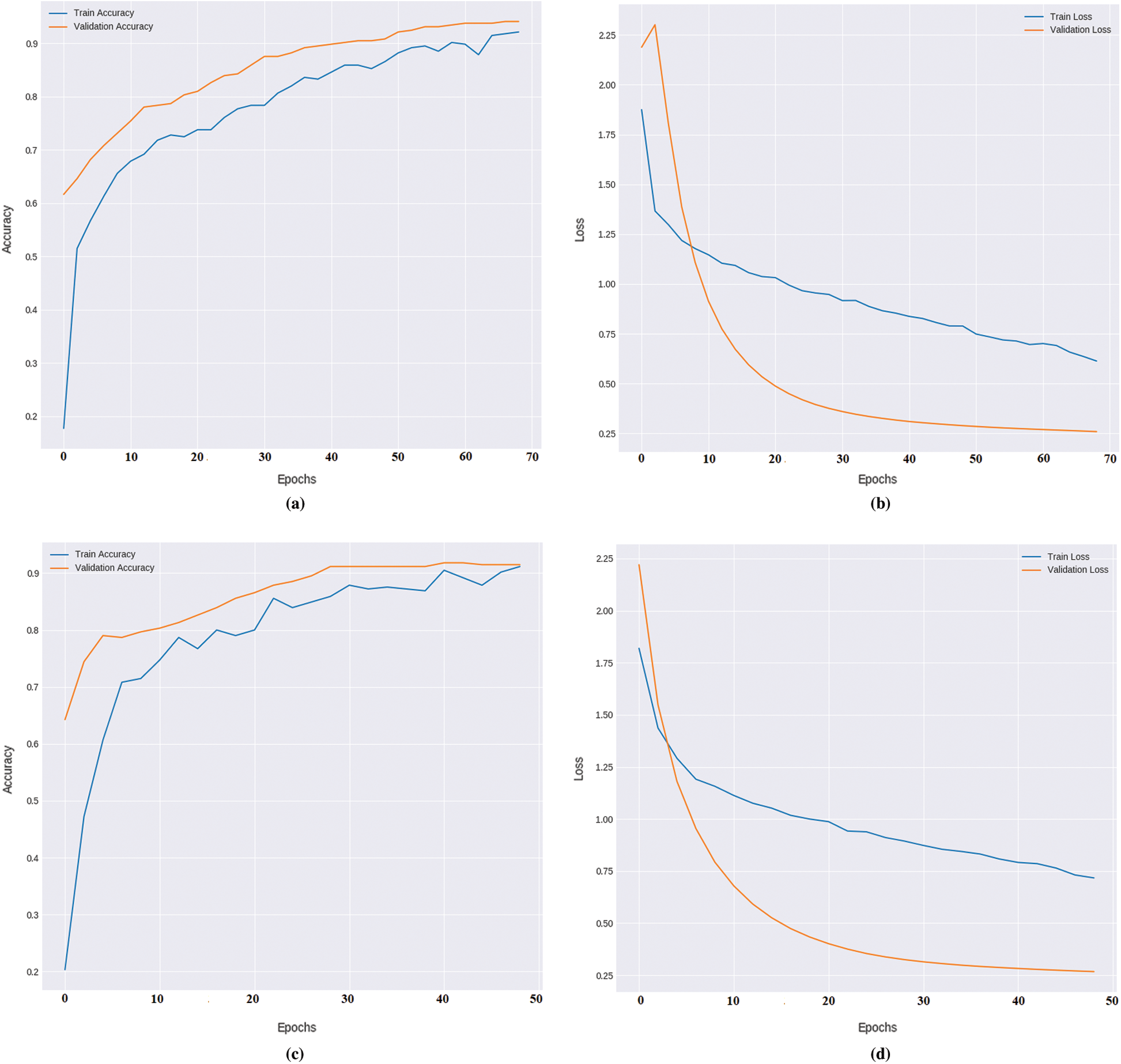
Figure 7: (a) Accuracy graph of India Pines dataset (b) loss graph of India Pines dataset (c) accuracy graph of Pavia University dataset (d) loss graph of Pavia University dataset
Particularly, the Xcep-HSIC model has reached a higher validation accuracy of 0.9432. Fig. 7b illustrates the loss graph analysis of the Xcep-HSIC model India Pines dataset. The loss graph tends to be decreased with an increase in epoch count, signifying the better performance of the Xcep-HSIC model interms of training and validation losses. Specifically, the Xcep-HSIC model reaches to the least validation loss of 0.27. Fig. 7c implies the accuracy graph of the Xcep-HSIC approach on the applied Pavia University dataset under various counts of epochs. The figure depicted that the training and validation accuracies are enhanced with maximization in the count of epochs. Ultimately, the Xcep-HSIC method has attained maximum validation accuracy of 0.9267. Fig. 7d demonstrates the loss graph examination of the Xcep-HSIC scheme Pavia University dataset. The loss graph is reduced by increased epoch value which denotes the better function of the Xcep-HSIC framework with respect to training and validation losses. Particularly, the Xcep-HSIC technique accomplishes a minimum validation loss of 0.275.
Tab. 3 provides a detailed comparative study of the results attained by the Xcep-HSIC model with existing methods [23,24] on the applied two dataset interms of accuracy and testing time. The value of accuracy needs to be high and testing time needs to be low for effective HSI classification outcome.
Table 3: Result analysis of existing with proposed Xcep-HSIC methods
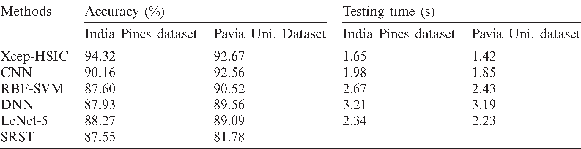
Fig. 8 investigates the HSI classification outcome of the Xcep-HSIC model on the applied dataset in terms of accuracy. On the classification of the India Pines dataset, the figure reported that the SRST model has led to poor HSI classification outcomes by obtaining a minimal accuracy of 87.55%. Likewise, the RBF-SVM method has resulted in a somewhat superior and closer accuracy of 87.6%. Eventually, the DNN model has tried to outperform the earlier models with a moderate accuracy of 87.93%. Simultaneously, the LeNet-5 model has revealed a slightly better HSI classification outcome with an accuracy of 88.27% whereas the near-optimal accuracy of 90.13% has been obtained by the CNN model. At last, the proposed Xcep-HSIC model has outperformed other HSI classifiers with a maximum accuracy of 94.32%. On the classification of the Pavia University dataset, the figure illustrated that the SRST approach has resulted in inferior HSI classification result by accomplishing the least accuracy of 81.78%. Likewise, the LeNet-5 framework has implied a considerable and closer accuracy of 89.09%. Followed by, the DNN method has attempted to surpass the traditional approaches with an acceptable accuracy of 89.56%. At the same time, the RBF-SVM technology has exhibited moderate HSI classification results with the accuracy of 90.52% while the closer optimal accuracy of 92.56% was achieved by the CNN scheme. Eventually, the proposed Xcep-HSIC model has outperformed other HSI classifiers with a maximum accuracy of 92.67%.
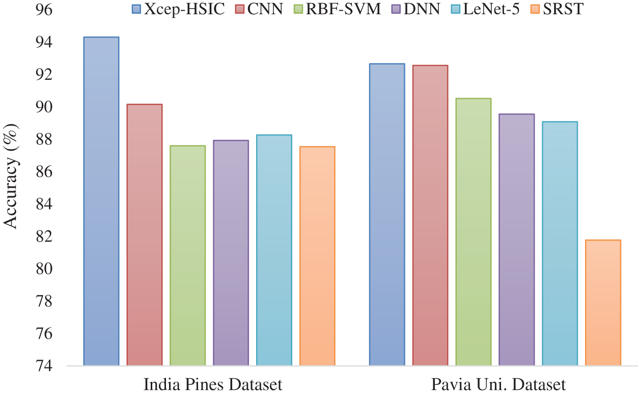
Figure 8: The accuracy analysis of Xcep-HSIC model
Fig. 9 analyzes the testing time of the proposed Xcep-HSIC model with the compared methods on the India Pines and Pavia university dataset. During the classification of the India Pines dataset, the figure showed that the DNN model requires a maximum testing time of 3.21 s, which is ignorantly higher than the other methods. Followed by, the RBF-SVM model has reached a slightly lower testing time of 2.67 s whereas an even lower testing time of 2.34 s has been needed by the LeNet-5 model. On continuing with, the CNN model has achieved a competitive outcome with an acceptable testing time of 1.98 s. But the proposed Xcep-HSIC model has demonstrated effective classification results with a minimum testing time of 1.65 s. In the classification of the Pavia university dataset, the figure demonstrated that the DNN scheme needs high testing time of 3.19 s that is higher than compared approaches. Besides, the RBF-SVM framework has attained a moderate testing time of 2.43 s while an even lower testing time of 2.23 s is required by the LeNet-5 technology. In line with this, the CNN technique has accomplished competing results with a considerable testing time of 1.85 s. However, the newly presented Xcep-HSIC method has showcased efficient classification outcomes with a lower testing time of 1.42 s.
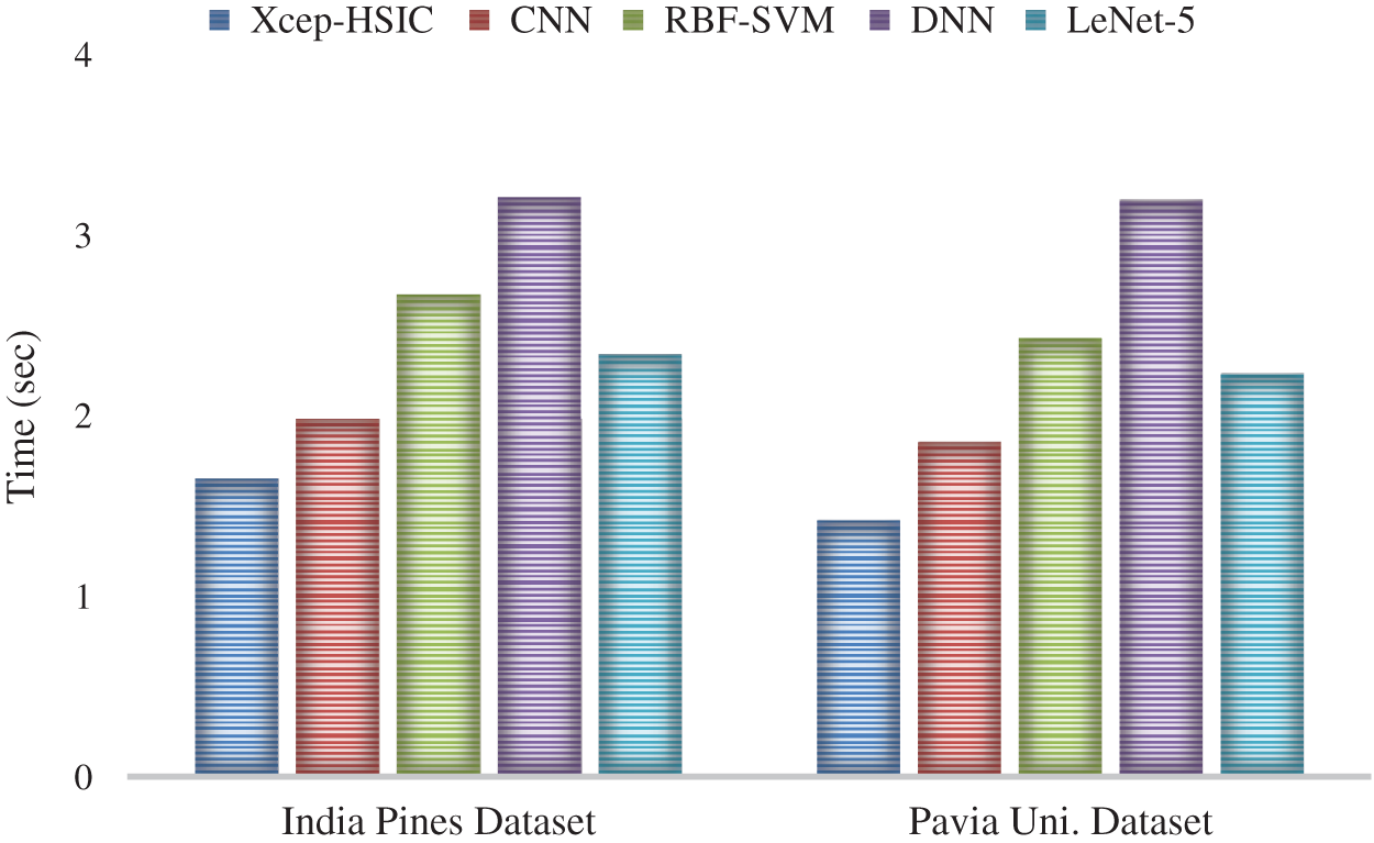
Figure 9: The testing time analysis of Xcep-HSIC model
The above-mentioned experimental results analysis showcased that the Xcep-HSIC model has been found as an effective HSI classification model to identify the distinct classes of HSI. The Xcep-HSIC model has reached a maximum accuracy of 94.32% and 92.67% on the applied India Pines and Pavia University dataset respectively.
This paper has developed a new model for HSI analysis and classification using the Xcep-HSIC model. The Xcep-HSI model performs the FRML map extraction process and then Xception based feature extraction task takes place to derive a set of feature vectors. At last, QPSO-KELM model is applied to identify the different class labels of HSI. In order to determine the parameters of KELM, the QPSO algorithm is introduced which helps to increase the overall classification performance. An extensive range of experiments was performed on two benchmark HSI dataset namely Indian Pines and Pavia University dataset. The simulation outcome verified the supremacy of the Xcep-HSIC technique over the existing methods with the maximum accuracy of 94.32% and 92.67% on the applied India Pines and Pavia University dataset. In future, the performance of the Xcep-HSIC model can be improved using parameter tuning strategies for the Xception model.
Funding Statement: The authors received no specific funding for this study.
Conflicts of Interest: The authors declare that they have no conflicts of interest to report regarding the present study.
1. M. Y. Teng, R. Mehrubeoglu, S. A. King, K. Cammarata and J. Simons. (2013). “Investigation of epifauna coverage on seagrass blades using spatial and spectral analysis of hyperspectral images,” in 2013 5th Workshop on Hyperspectral Image and Signal Processing: Evolution in Remote Sensing, Gainesville, FL, USA, IEEE, pp. 1–4. [Google Scholar]
2. F. Ratle, G. C. Valls and J. Weston. (2010). “Semisupervised neural networks for efficient hyperspectral image classification,” IEEE Transactions on Geoscience and Remote Sensing, vol. 48, no. 5, pp. 2271–2282. [Google Scholar]
3. G. E. Hinton and R. R. Salakhutdinov. (2006). “Reducing the dimensionality of data with neural networks,” Science, vol. 313, no. 5786, pp. 504–507. [Google Scholar]
4. S. Zhou, Z. Xue and P. Du. (2019). “Semisupervised stacked autoencoder with cotraining for hyperspectral image classification,” IEEE Transactions on Geoscience and Remote Sensing, vol. 57, no. 6, pp. 3813–3826. [Google Scholar]
5. P. Dou and C. Zeng. (2020). “Hyperspectral image classification using feature relations map learning,” Remote Sensing, vol. 12, no. 18, pp. 1–25. [Google Scholar]
6. Y. Chen, Z. Lin, X. Zhao, G. Wang and Y. Gu. (2014). “Deep learning-based classification of hyperspectral data,” IEEE Journal of Selected Topics in Applied Earth Observations and Remote Sensing, vol. 7, no. 6, pp. 2094–2107. [Google Scholar]
7. Y. Chen, X. Zhao and X. Jia. (2015). “Spectral–spatial classification of hyperspectral data based on deep belief network,” IEEE Journal of Selected Topics in Applied Earth Observations and Remote Sensing, vol. 8, no. 6, pp. 2381–2392. [Google Scholar]
8. C. Ding, Y. Li, Y. Xia, W. Wei, L. Zhang et al. (2017). , “Convolutional neural networks based hyperspectral image classification method with adaptive kernels,” Remote Sensing, vol. 9, no. 6, pp. 1–15. [Google Scholar]
9. H. Wu and S. Prasad. (2017). “Convolutional recurrent neural networks for hyperspectral data classification,” Remote Sensing, vol. 9, no. 3, pp. 1–20. [Google Scholar]
10. W. Li, G. Wu, F. Zhang and Q. Du. (2017). “Hyperspectral image classification using deep pixel-pair features,” IEEE Transactions on Geoscience and Remote Sensing, vol. 55, no. 2, pp. 844–853. [Google Scholar]
11. B. Pan, Z. Shi and X. Xu. (2017). “A new deep-learning-based hyperspectral image classification method,” IEEE Journal of Selected Topics in Applied Earth Observations and Remote Sensing, vol. 10, no. 5, pp. 1975–1986. [Google Scholar]
12. M. Zhang, W. Li and Q. Du. (2018). “Diverse region-based CNN for hyperspectral image classification,” IEEE Transactions on Image Processing, vol. 27, no. 6, pp. 2623–2634. [Google Scholar]
13. X. Ceamanos, B. Waske, J. A. Benediktsson, J. Chanussot, M. Fauvel et al. (2010). , “A classifier ensemble based on fusion of support vector machines for classifying hyperspectral data,” International Journal of Image and Data Fusion, vol. 1, no. 4, pp. 293–307. [Google Scholar]
14. X. Huang and L. Zhang. (2012). “An SVM ensemble approach combining spectral, structural, and semantic features for the classification of high-resolution remotely sensed imagery,” IEEE Transactions on Geoscience and Remote Sensing, vol. 51, no. 1, pp. 257–272. [Google Scholar]
15. Y. Gu and H. Liu. (2016). “Sample-screening MKL method via boosting strategy for hyperspectral image classification,” Neurocomputing, vol. 173, pp. 1630–1639. [Google Scholar]
16. C. Qi, Z. Zhou, Y. Sun, H. Song, L. Hu et al. (2017). , “Feature selection and multiple kernel boosting framework based on PSO with mutation mechanism for hyperspectral classification,” Neurocomputing, vol. 220, pp. 181–190. [Google Scholar]
17. M. Turkoglu, D. Hanbay and A. Sengur. (2019). “Multi-model LSTM-based convolutional neural networks for detection of apple diseases and pests,” Journal of Ambient Intelligence and Humanized Computing, vol. 15, no. 1, pp. 1–11. [Google Scholar]
18. M. Mahdianpari, B. Salehi, M. Rezaee, F. Mohammadimanesh and Y. Zhang. (2018). “Very deep convolutional neural networks for complex land cover mapping using multispectral remote sensing imagery,” Remote Sensing, vol. 10, no. 7, pp. 1–21. [Google Scholar]
19. Y. Zhang, X. Jiang, X. Wang and Z. Cai. (2019). “Spectral–spatial hyperspectral image classification with superpixel pattern and extreme learning machine,” Remote Sensing, vol. 11, no. 17, pp. 1–20. [Google Scholar]
20. J. Liu, J. Sun and W. B. Xu. (2006). “Design IIR digital filters using quantum-behaved particle swarm optimization,” Advances in Natural Computation, Lecture Notes in Computer Science, vol. 4222, pp. 637–640. [Google Scholar]
21. D. Yumin and Z. Li. (2014). “Quantum behaved particle swarm optimization algorithm based on artificial fish swarm,” Mathematical Problems in Engineering, vol. 2014, pp. 1–10. [Google Scholar]
22. “The Real HYDICE Urban Hyperspectral Dataset. Available online: http://lesun.weebly.com/hyperspectraldata-set.html (accessed on 13 June 2019). [Google Scholar]
23. W. Hu, Y. Huang, L. Wei, F. Zhang and H. Li. (2015). “Deep convolutional neural networks for hyperspectral image classification,” Journal of Sensors, vol. 2015, no. 2, pp. 1–12. [Google Scholar]
24. Y. Wu, G. Mu, C. Qin, Q. Miao, W. Ma et al. (2020). , “Semi-supervised hyperspectral image classification via spatial-regulated self-training,” Remote Sensing, vol. 12, no. 1, pp. 1–20. [Google Scholar]
 | This work is licensed under a Creative Commons Attribution 4.0 International License, which permits unrestricted use, distribution, and reproduction in any medium, provided the original work is properly cited. |