DOI:10.32604/cmc.2021.015424
| Computers, Materials & Continua DOI:10.32604/cmc.2021.015424 | |
| Article |
Weighted Gauss-Seidel Precoder for Downlink Massive MIMO Systems
1Department of Information and Communication Engineering, Convergence Engineering for Intelligent Drone, Sejong University, Seoul, 05006, Korea
2Department of Computer Engineering, Sejong University, Seoul, 05006, Korea
*Corresponding Author: Hyoung-Kyu Song. Email: songhk@sejong.ac.kr
Received: 20 November 2020; Accepted: 12 December 2020
Abstract: In this paper, a novel precoding scheme based on the Gauss-Seidel (GS) method is proposed for downlink massive multiple-input multiple-output (MIMO) systems. The GS method iteratively approximates the matrix inversion and reduces the overall complexity of the precoding process. In addition, the GS method shows a fast convergence rate to the Zero-forcing (ZF) method that requires an exact invertible matrix. However, to satisfy demanded error performance and converge to the error performance of the ZF method in the practical condition such as spatially correlated channels, more iterations are necessary for the GS method and increase the overall complexity. For efficient approximation with fewer iterations, this paper proposes a weighted GS (WGS) method to improve the approximation accuracy of the GS method. The optimal weights that accelerate the convergence rate by improved accuracy are computed by the least square (LS) method. After the computation of weights, the different weights are applied for each iteration of the GS method. In addition, an efficient method of weight computation is proposed to reduce the complexity of the LS method. The simulation results show that bit error rate (BER) performance for the proposed scheme with fewer iterations is better than the GS method in spatially correlated channels.
Keywords: Massive MIMO; GS; matrix inversion; complexity; weight
Massive multiple-input multiple-output (MIMO) for a very large scale of multi-user (MU) MIMO is a significant technology that enables advancement to the fifth-generation (5G) cellular networks. Since hundreds of antennas at the base station (BS) induce significant multiplexing and diversity gain, massive MIMO systems provide high energy efficiency, spectral efficiency, and transmit reliability compared with small scale MU-MIMO systems. Also, simple linear processing such as the ZF method provides optimal performance by the channel hardening property that makes fading channels behave as deterministic channels in massive MIMO systems. It has been proved that the ZF method with accurate channel state information (CSI) can perfectly eliminate intra-cell interference (ICI) in a single-cell system [1–6]. Indeed, there are various non-linear processing methods and those provide higher error performance than linear processing methods [7]. However, the complexity of non-linear processing as an existing problem has become higher in large scale MIMO systems. Therefore, the ZF method as the simple linear processing with optimal performance has been attracted attention for massive MIMO systems [5]. However, the ZF method requires the operation of direct matrix inversion whose computational complexity for multiplication is  where Nu is the number of users. The complexity of direct matrix inversion is unaffordable for the practical implementation of massive MIMO systems which serve tens of users as the number of BS antennas increases [6]. Several precoding and detection schemes with low complexity were surveyed in [8–11]. To balance between the complexity and performance, many studies that approximate the matrix inversion to reduce the complexity were conducted [12–24], and approximate methods can be classified into two categories: Neumann series expansion (NSE) and iterative method.
The NSE method approximates the matrix inversion as expansion terms of a matrix polynomial. The invertible matrix for an initial matrix is required to use the NSE method. The diagonal matrix was used as the initial matrix of the NSE method to achieve the error performance equivalent to the ZF method and low complexity in [12,13]. However, the NSE method has two limited conditions related to its practical application to massive MIMO systems. Firstly, the expansion of the NSE method does not exceed 2 terms since the expansion of 3 terms requires the same complexity of  as direct matrix inversion. Secondly, the NSE method can only achieve high convergence probability in the large ratio
  , where the ratio
  is defined as
  and Nb is the number of BS antennas [13]. Thus, the NSE method is difficult to achieve both low complexity and high approximation accuracy in small
  .
.
To obtain better approximation accuracy than the NSE method for the same complexity, the iterative method approximates a vector multiplied by an invertible matrix. Since the iterative method only requires matrix-vector multiplication operation, any iterations maintain the complexity of  . The error performance of iterative methods is determined depending on the initial solution and iteration matrix. The GS method requires fewer iterations for demanded error performance compared with other iterative methods such as Jacobi et al. [9].
To improve the error performance of the GS method, the initial solutions were variously defined in [15–19]. The stair matrix was proposed as the initial solution in [15]. The one expansion term of the NSE method that uses the diagonal matrix as the initial matrix was proposed as the initial solution in [16]. Also, the two expansion terms of the NSE method were proposed as the initial solution in [17–19]. In addition to variant initial solutions, the successive over relaxation (SOR) methods that converge faster with the aid of a relaxation parameter compared with the GS method were proposed in [20–22]. The GS and SOR methods can converge to the error performance of the ZF method with fewer iterations under the ideal conditions such as the large  . However, the convergence rate and approximation accuracy are reduced under practical conditions such as the small
  and spatially correlated channels. To solve these problems, the GS methods based on the soft-output detector for uplink systems were proposed in [16–18], and the SOR method applying adaptive relaxation parameters for each iteration was proposed in [22]. Another way to solve these problems applies different weights for each expansion term or iteration to improve the error performance. The NSE methods applying different weights were proposed in [23,24], and the approximate methods with properly computed weights can achieve better error performance. However, References [12–22] did not consider the performance improvement by weighting, and the weights for each iteration were only set to default value as 1. In addition to weighting the approximate method, the consideration of practical channel environment is significant in terms of performance verification [6]. This paper especially verifies the error performance of iterative methods for spatially correlated channels.
In this paper, a WGS method to perform the ZF precoder is proposed and provides better error performance in spatially correlated channels. The weights that minimize the error between exact and approximate matrix inversion are computed by the LS method. For a feasible LS method, the process of the GS method should be transformed into the form of NSE. The optimal weights are only computed by the channel response of each channel coherence interval. However, the proposed scheme uses one weight vector in the optimal weights since it is more efficient in terms of computational complexity. Also, this paper proposes an efficient method to reduce the complexity for the computation of the weights. The simulation results show that the WGS precoder provides better error performance than the GS precoder.
This paper is organized as follows. Section 2 presents models for the downlink massive MIMO system and spatially correlated channels. Section 3 explains iterative methods, the GS precoder, and the improvement of the GS method. In Section 4, the WGS precoder and the efficient weight computation method are proposed. Also, Section 4 provides the computational complexity for iterative methods. Section 5 presents the simulation results for BER performance comparison of iterative methods. Finally, Section 6 gives brief conclusions.
This section presents a downlink massive MIMO system model and channel model assumed in this paper.
2.1 Downlink Massive MIMO System Model
Fig. 1 shows the system configuration for the downlink massive MIMO where the BS with Nb transmit antennas simultaneously communicates Nu users with a single antenna, and  is assumed. The channel matrix
  between all transmit antennas and total users is
  whose the m-th row vector is
  . The received symbol ym at the m-th user is as follows:

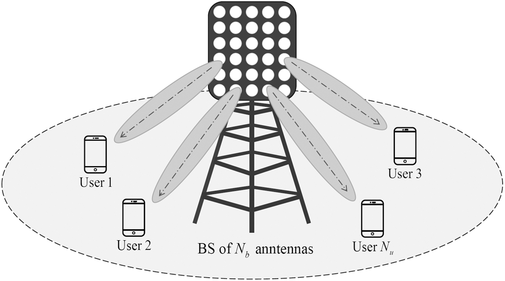
Figure 1: The downlink massive MIMO system configuration
where P is the downlink transmit power,  is an
is an  precoding matrix,
  is the m-th column of
  , sm is the m-th complex transmit symbol with zero mean and unit variance, zm is the m-th additive white Gaussian noise (AWGN) with zero mean and unit variance, and
  is Frobenius norm operator.
For spatially correlated channels, this paper considers the exponential correlation matrix model which is expressed as [25]

where ri, j is the element in the i-th row and j-th column of the spatial correlation matrix  ,
,  is the complex conjugate,
  is the correlation coefficient,
  is the correlation coefficient magnitude with
  , and
, and  is randomly determined in interval
  . The channel matrix
  is expressed as follows:

where  is an
is an  Rayleigh fading channel matrix which elements are independent and identically distributed (i.i.d.) circular symmetric complex Gaussian random variables with zero mean and unit variance,
  is an
is an  complex spatial correlation matrix for receive antennas, and
  is an
is an  complex spatial correlation matrix for transmit antennas. The distance between adjacent antennas is related to the correlation coefficient magnitude and the larger distance than half a wavelength can omit the spatial correlation [22]. This paper considers single antenna users and assumes that the distance of users is larger than half a wavelength. Therefore, it is assumed that the magnitude of correlation coefficient of the user has zeros in this paper.
In this section, iterative methods and the relationship between iterative method and NSE are briefly explained, and the GS precoders are presented.
The iterative method approximates a signal vector  to solve the linear equation of
  . The iterative method can be expressed as follows:

where  ,
,  is a nonsingular matrix, subscript k is the iteration number, and
  is an initial solution that generally assumes zero vector. The expression of Eq. (4) with respect to the
  is expressed as follows:

where  is an iteration matrix. For the convergence of
  , the condition of
  should be satisfied, and
  is the spectral radius of a matrix. In comparison to the iterative method, the NSE method is expressed as follows:

where  is the
  identity matrix, and the iterative method can be transformed as the form of NSE as follows:

where the initial solution  is zero vector, and the M is called as preconditioner that determines the error performance of approximate methods.
For the expression of the GS precoder, the gram matrix  is defined as follows:

The preconditioner of the GS method is expressed as follows:

where  is decomposed as
  ,
,  is the diagonal part,
  is the strictly lower part, and
  is the strictly upper part. The k-th GS solution
  is calculated as follows:

where  is a
is a  modulated symbol vector. The downlink transmit symbol vector
  is calculated with matched filter as follows:

where  is scaling factor to normalize the total transmit power.
The initial solution  is variously defined according to the system requirement, which can improve the convergence rate and approximation accuracy of iterative methods. Among various initial solutions, the recent initial solution for improvement of the GS method is expressed as [18]

where the matrix  is defined as
  . Another way to improve the GS method is the usage of a relaxation parameter. The relaxation parameter
  to the GS method to work well at any
  is applied as [19]

Eq. (13) is called as the SOR method, and the GS method is special case of the SOR method whose the value of  is equal to 1. The GS precoder with the initial solution of Eq. (12) and the SOR precoder with the appropriately selected
  provides better error performance than the GS precoder with the initial solution of zero vector.
4 Proposed Downlink Precoding Scheme
In Section 2, the spatially correlated channel is considered. The problem is that the spatial correlation degrades the error performance of approximate methods. Although direct elimination of the spatial correlation is difficult, the improvement of error performance can alleviate this problem to some extent. In this section, a WGS method is designed to improve the error performance of the GS precoder for downlink massive MIMO systems. The WGS method is inspired by the weighted Neumann series in [23,24]. Also, an efficient method to reduce the complexity of weight computation is proposed.
The proposed scheme that applies different weights to each iteration of the GS method is expressed as follows:

where  are complex weights to decrease approximation error, and the initial solution
  is zero vector. For the computation of the optimal weights, the WGS method is expressed similarly with Eq. (6) as follows:

where the weights are applied in reverse order to each term of matrix polynomial, and the weighted  of the GS method is expressed as follows:

where an is the weight of reverse order to simplify the subscript. The weights can be computed by the LS method that determines the solution of the linear model in which the given data is the channel response [26]. Firstly, the optimal weights should minimize the value of the problem as follows:

For the computation of the optimal weights, the j-th term of the matrix polynomial of the  except the weight parameter is defined as follows:

where  is the
  -th column vector of
  and the
  -th column vector of
  is defined as
  . Secondly, the optimization problem in Eq. (17) can be modified with the different form that computes the weights as the solution of linear equation. The modified optimization problem is defined as follows:

where  is a
is a  weight vector
  is the
  vector, and
  is a
is a  combined matrix whose the
  -th element is
  as follows:

Finally, the weight vector computed by the LS method is expressed as follows:

In this way, the computation of the optimal weights should be performed at every channel coherence interval, and the computational complexity is higher than direct matrix inversion. To reduce the complexity, the WGS precoder uses the only one optimal weight vector computed early in the system. The computation of the weights is executed only once and not included in approximation complexity. Since the optimal weights are determined only within a certain distribution, any weights in the distribution can sufficiently improve the error performance of the GS precoder. Fig. 2 shows the distribution of the optimal weights for 5 expansion terms of matrix polynomial in complex plane. To illustrate the effect of the spatial correlation and the ratio  on weights, three different cases are presented. In Fig. 2, n is the order of the weights, the Nb is fixed at 200. The case (a) is that Nu is 20 and
  is 0, the case (b) is that Nu is 40 and
  is 0, and the case (c) is that Nu is 40 and
  is 0.3. The number of optimal weights representing the distribution is 200 for each term of the matrix polynomial. The distribution of the case (c) is the largest in Fig. 2, but is enough small since the width of the distribution for real and imaginary values is close to 1. The optimal weights change according to the
  and
and  since the correlation degree of the channels is different. The weights of the first and second order overlap since those values are close to 1. In contrast, the absolute value of the weights for the latter order increases as the correlation degree of the channels increases and is clearly observed.
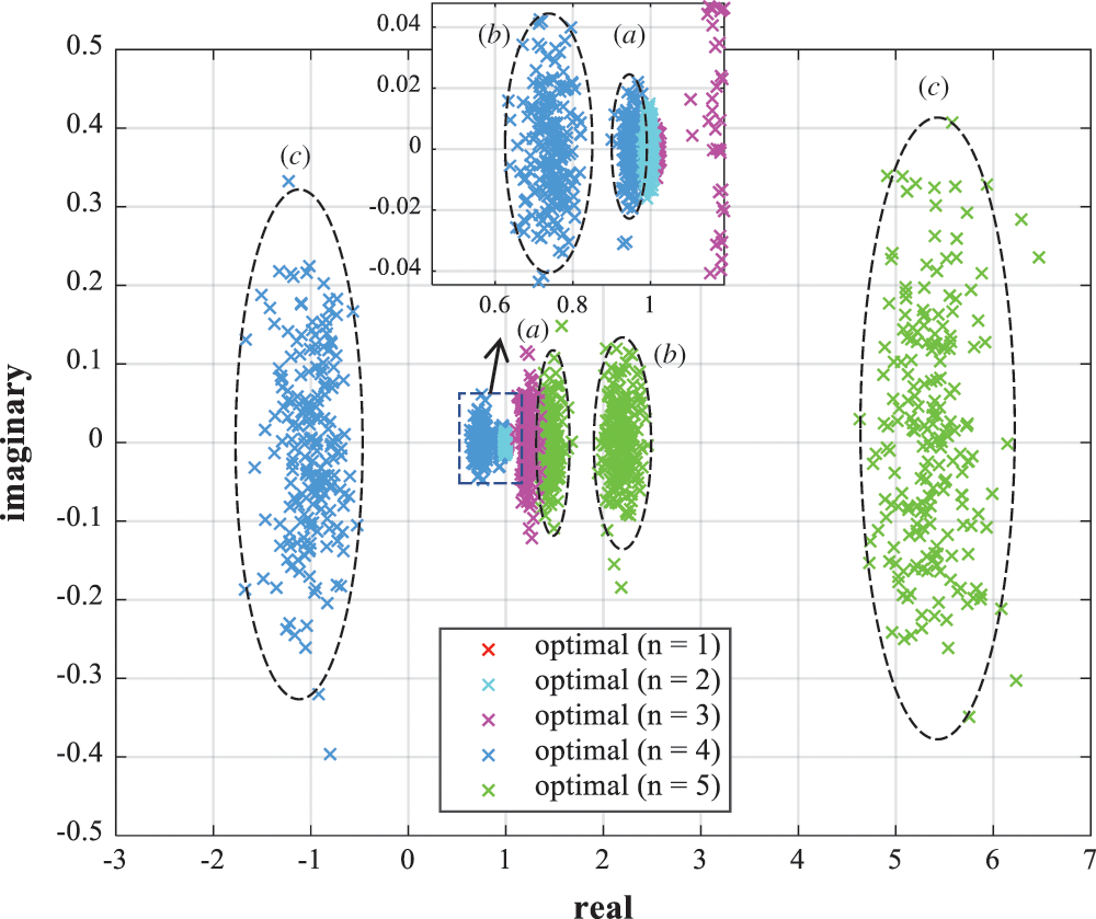
Figure 2: The distribution of optimal weights in three different cases
4.2 Efficient Weight Computation Method
As seen above process, the LS method can efficiently compute the weights. However, the computation method of the optimal weights requires very high computational complexity  . This paper proposes an efficient method to compute the weights with less complexity. The complexity can be reduced by modifying the
  and
and  in Eq. (21). The modified
  is defined as the
  combined matrix X as follows:

where  forms the diagonal elements of a matrix to a column vector, and the modified
  is defined as the
  vector
  whose all elements have the value of 1. The efficient weight computation method is expressed similarly with Eq. (21) as follows:

Additionally, only the real part of the weights is used to exclude the influence on imaginary values when the weights are determined close to the distribution boundary on the imaginary axis. In terms of the number of users, the weight computation method using only the diagonal elements for each term of the matrix polynomial reduces the complexity to  . The weights computed by Eq. (23) are close enough to the optimal weights and significantly improve the error performance of the GS method. Tab. 1 expresses the meaning of parameters in the WGS algorithm that the summary of the WGS precoder using the real part of one
  is expressed as an algorithm as follows:
Step 1: Input parameter 
Step 2: Initialization

Step 3: Weight computation

for 
end for

Step 4: GS iteration
for 

end for
Step 5: GS precoder

Step 6: Output parameter 
Table 1: The meaning of parameters in the WGS algorithm

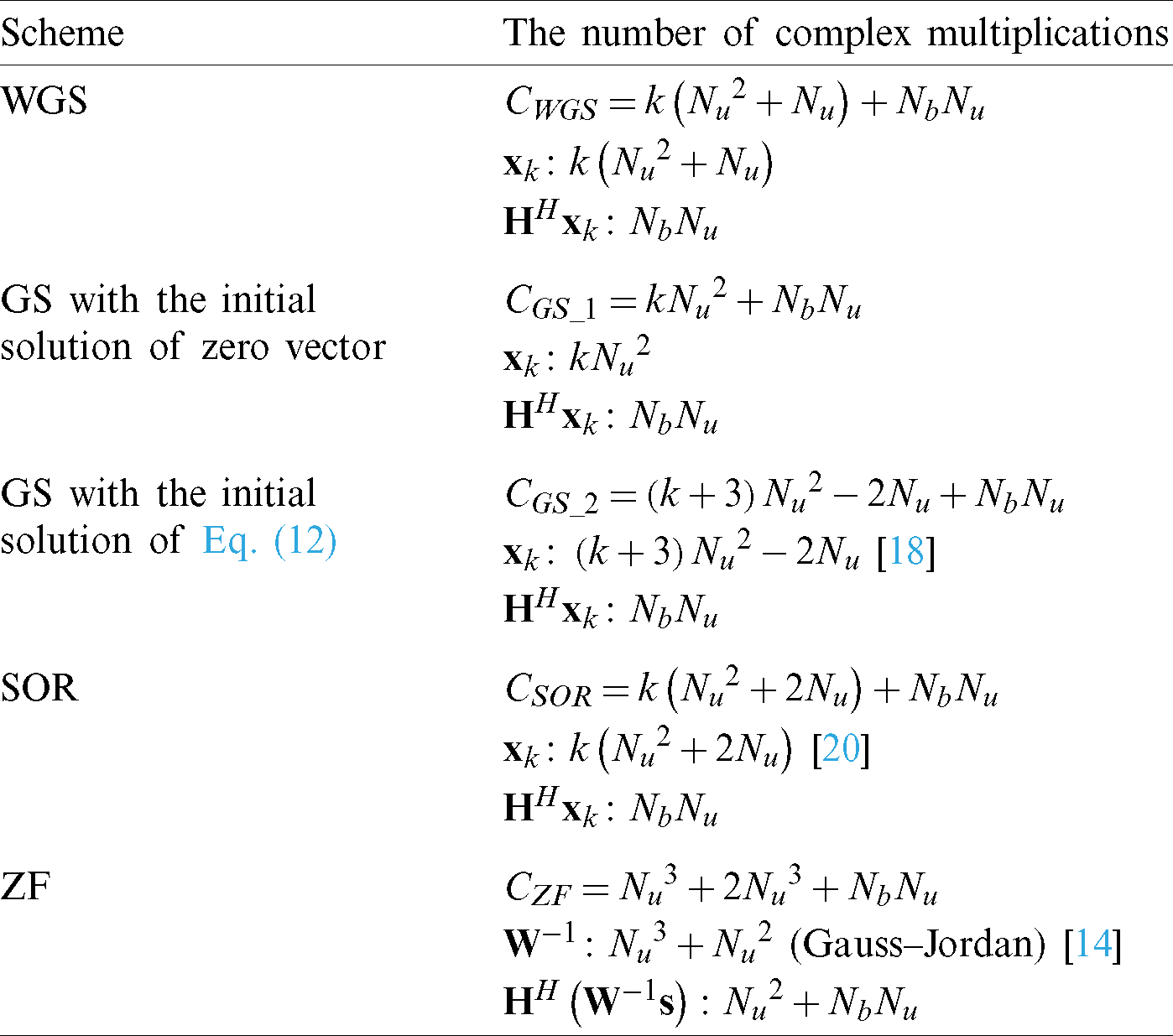
Tab. 2 expresses the complexity of iterative precoders compared in simulation results. The number of complex multiplications for only calculating  is considered, and the complexity of the weight computation is excluded since the weight vector is not iteratively computed during the precoding process. The difference between the WGS and the GS method is the application of the weights as a coefficient of symbol vector in Eq. (14). The
  of the WGS method is expressed in terms of elements as follows:

where  ,
,  , and si are the i-th element of
  ,
,  , and
, and  respectively, and
  is the element in the i-th row and j-th column of
  . The multiplication required for one element of
  can be divided as 4 parts. The number of multiplications outside parenthesis is 1. In parenthesis, The number of multiplications for the first term is 1, the number of multiplications for the second term is i −1, and the number of multiplication for the third term is Nu − i. Since the size of
  is
is  , the total number of multiplications for one iteration is
  .
.
Table 2: The complexity of iterative precoders
5 Performance Evaluation and Discussion
In this section, the BER performances of iterative precoders according to signal to noise ratio (SNR) are presented. The BER performance of the exact ZF precoder is provided as a benchmark. To confirm the difference in weight usage for BER performance, the GS precoder with the initial solution of zero vector is compared with the WGS precoder. Also, the BER performances of the GS precoder with the initial solution of Eq. (12) and the SOR precoder are provided to compare with the WGS precoder. In all simulations, the number of antennas at BS is fixed at 200 while the number of users is 20, 30 and 40 respectively, and 64-quadrature amplitude modulation (QAM) is used. The downlink channels are modelled as the Rayleigh fading channel with or without spatial correlation. In simulation results,  indicates the iteration number.
Fig. 3 shows the comparison of the use of different weight vectors for the WGS method. The number of users is 30, the correlation magnitude is 0.5, and the number of iterations is 5. In Fig. 3, using all elements means the use of one  , using diagonal elements means the use of the real part of one
  , and optimal weights mean the use of optimal weight vector that changes at each coherence interval. Fig. 3a presents the distance between weight values computed once by other methods and optimal weight values in complex plane according to the weight order. In Fig. 3a, the distance is averaged by 1000 optimal weight vectors. The graph shape can be different depending on the weight vector which is computed once. However, the difference in the graph shape does not change significantly since the one weight vector is determined close to the certain distribution as shown Fig. 2. The distance value calculated by comparison with the one
  is smaller than using
  , and the distance value of
  on all weight order is smaller than 1. Furthermore, the BER performances are nearly same for all weight vectors in Fig. 3b. Thus, the use of
  for the WGS precoder is reasonable in terms of the complexity and the BER performance, and the weight vector of the WGS precoder presented in all of following simulation results is based on the real part of the
  .
.
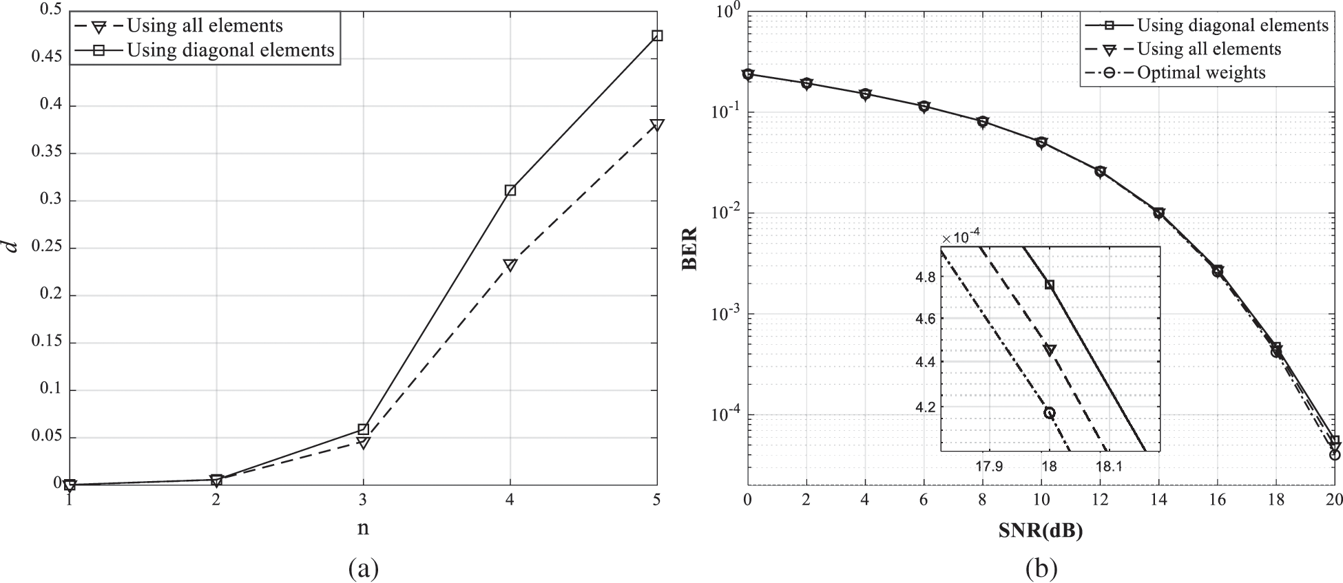
Figure 3: The comparison of using different weights in spatially correlated channel
Fig. 4 shows the average magnitude for the diagonal dominance of  according to the different number of users and correlation magnitude. The average magnitude for the diagonal dominance of
  is calculated as follows:

where wi, j is the element in the i-th row and j-th column of  . Since the low ratio
  and high correlation magnitude weaken the channel hardening property, the average magnitude for the diagonal dominance of
  is decreased.
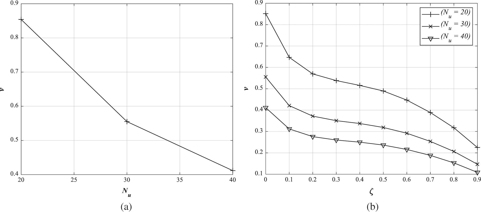
Figure 4: The average magnitude for diagonal dominance of  according to the different number of users and correlation magnitude
Fig. 5 shows the BER performances of the GS precoder with the initial solution of zero vector and the WGS precoder in ideal Rayleigh fading channel with no spatial correlation. In order to compare the WGS precoder with the GS precoder only with respect to the number of users, the number of users is chosen as 20, 30 and 40. For all number of users, the BER performance of the WGS precoder is close to the exact ZF precoder in 3 iterations. However, the WGS and GS precoders provide nearly the same BER performance as the exact ZF precoder in Fig. 5a since the ratio  is large. In Figs. 5b and 5c, the difference of 2 dB is shown in the range of 18–20 dB. The difference in the BER performances is increasingly clear as the number of users increases.
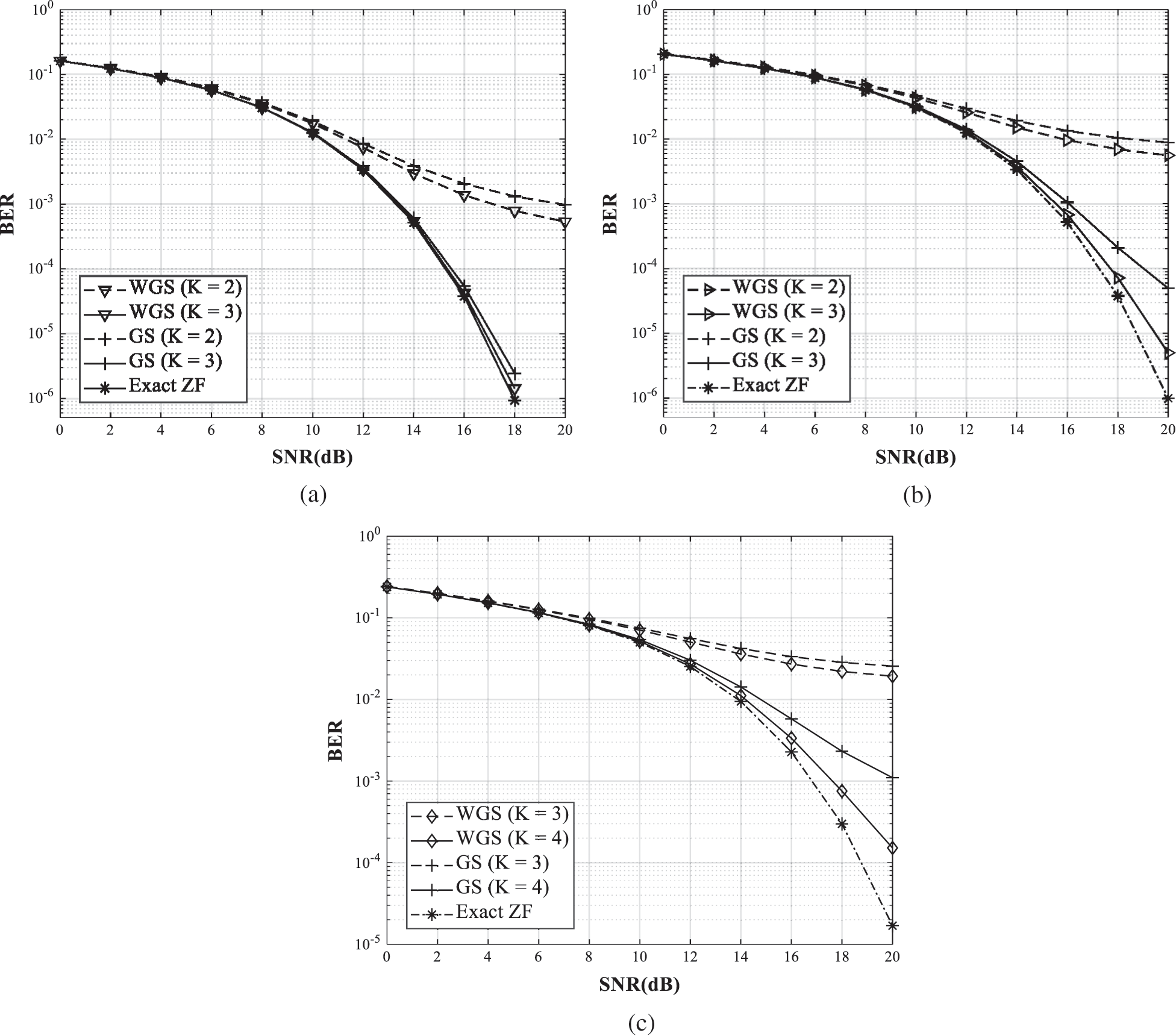
Figure 5: The BER performance comparison of the WGS, GS and exact ZF precoders in ideal Rayleigh fading channel with the different number of users. (a) Nb = 200, Nu = 20,  . (b) Nb = 200, Nu = 30,
  . (c) Nb = 200, Nu = 40,
Fig. 6 shows the BER performances of the GS precoder with the initial solution of zero vector and the WGS precoder in spatially correlated channel. The number of users is 20, and the correlation magnitude is 0.5. For  , the BER performance of the WGS precoder is close to the exact ZF precoder. The WGS precoder provides better BER performance than the GS precoder in the same iterations since the weights accelerate the convergence rate. The difference in the BER performances is more obvious compared with Fig. 5 since the spatial correlation significantly degrades the BER performance of the GS precoder.
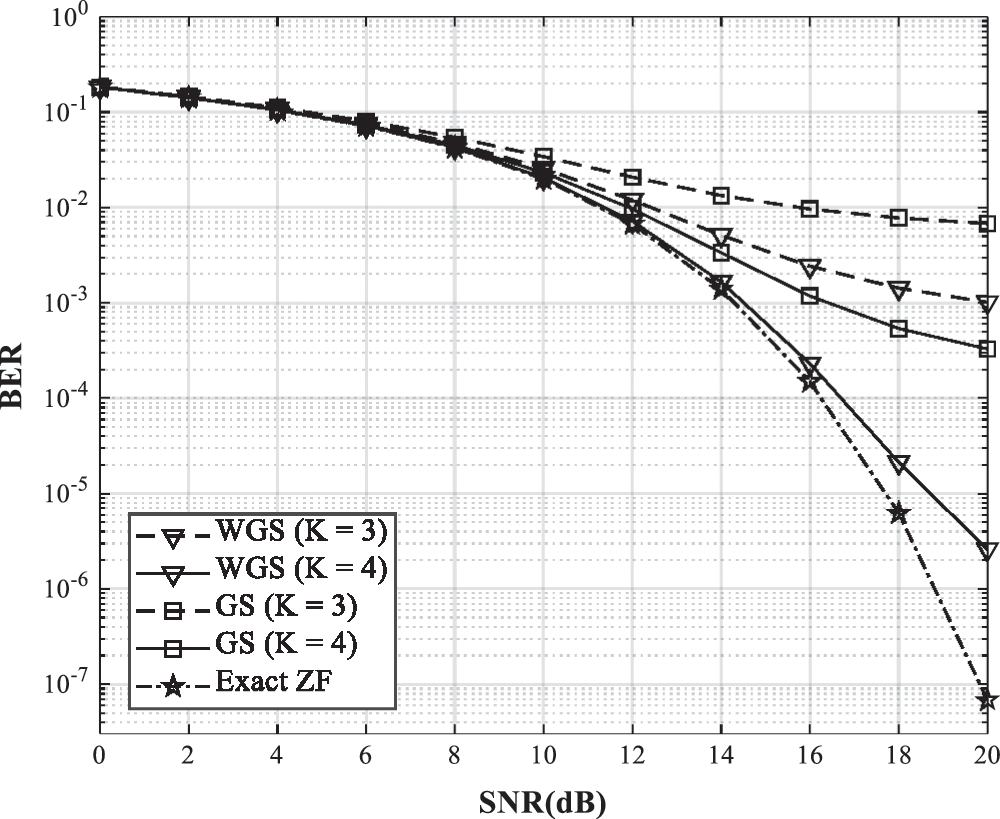
Figure 6: The BER performance comparison of the WGS, GS and exact ZF precoders in spatially correlated channel
Fig. 7 shows the difference of approximation accuracy and convergence rate for the iterative methods according to the iteration number. In Fig. 7a, the approximation error between  and
and  for the iterative methods is shown. The approximation error is calculated as follows:

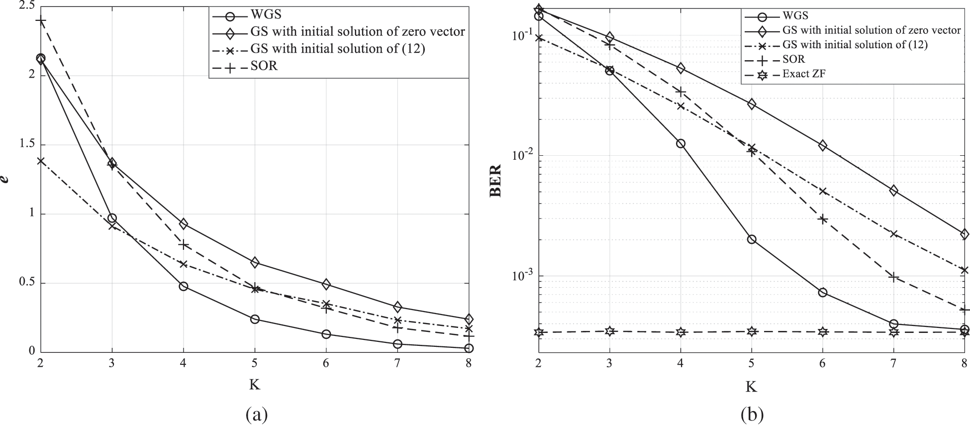
Figure 7: The approximation error and BER performances for the iterative methods according to the number of iterations
In Fig. 7b, the comparison of BER performances is shown for the SNR of 20 dB. The number of uses is 40, the correlation magnitude is 0.5, and the range of iterations is from 2 to 8 to clearly confirm that the error is gradually decreased and the WGS method completely convergences to the ZF method. The nearly optimal relaxation parameter of SOR method is empirically chosen for each configuration and correlation magnitude in Fig. 7 and following simulation results. It is confirmed that the graph shape in Fig. 7a is similar with that in Fig. 7b. Therefore, the decrease of the approximation error is directly related to the increase in BER performance. The WGS method shows the fastest convergence rate among the compared methods since the weights decrease the approximation error. Also, the approximation error and BER performance for WGS method with  are smaller than other methods with
  .
.
Fig. 8 shows the BER performance for the WGS precoder, the GS precoder with the initial solution of zero vector, the GS precoder with the initial solution of Eq. (12), and the SOR precoder. In order to clarify the difference in BER performance among iterative precoders, the range of SNR is increased by 2 dB and 4 dB respectively. The correlation magnitude is fixed at 0.5, and the number of users is 30 and 40. In this situation, the WGS precoder requires more iteration to approach the BER performance of the exact ZF precoder since the convergence rate is sufficiently decreased. However, the WGS precoder outperforms the GS precoder with the initial solution of zero vector. In Fig. 8a, the WGS precoder is close to the exact ZF precoder in 5 iterations, and the WGS precoder provides better BER performance than the other iterative precoders in the same iterations. In Fig. 8b, the WGS precoder is close to the exact ZF precoder in 6 iterations, and even the WGS precoder with 5 iterations provides better BER performance than the other iterative precoders with 6 iterations.
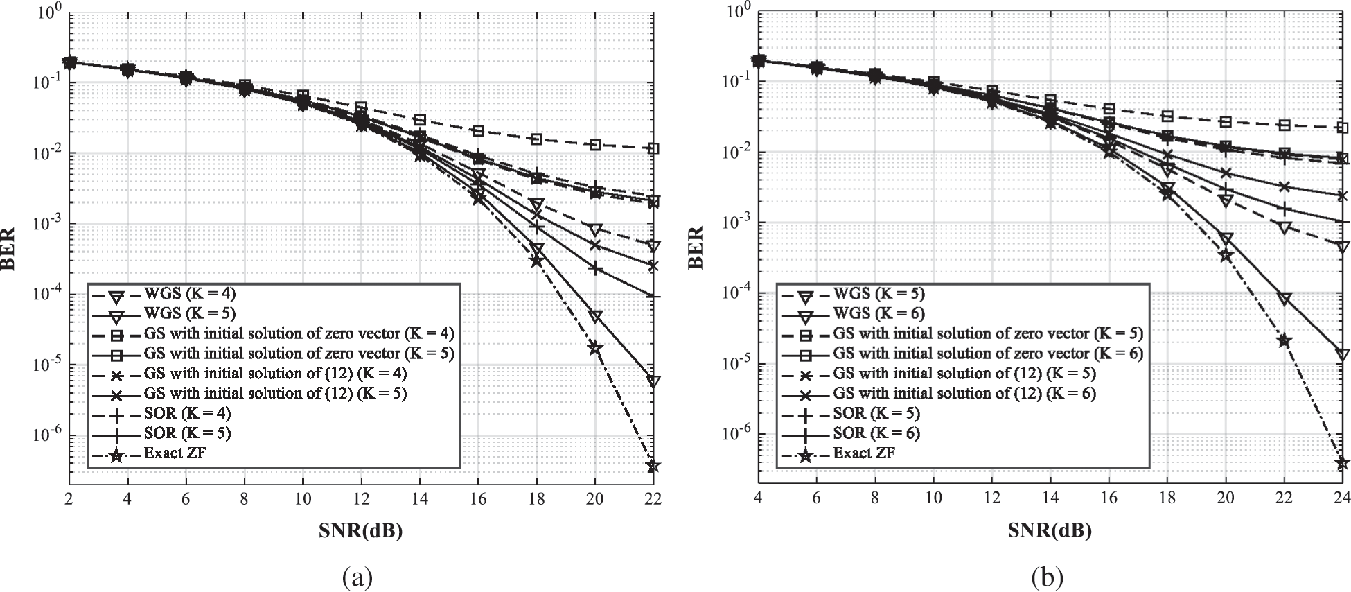
Figure 8: The BER performance comparison of the iterative precoders and the exact ZF precoders in spatially correlated channel with the different number of users. (a) Nb = 200, Nu = 30,  . (b) Nb = 200, Nu = 40,
The improvement of the BER performance for the WGS precoder is noticeable in the large ratio  and spatially correlated channels. The WGS precoder maintains a faster convergence rate than the other iterative precoders, but large number of iterations can be required to converge to the BER performance of the exact ZF precoder shown in Fig. 8. However, the overall complexity is decreased by reducing the iteration number to satisfy demanded BER performance. In addition, the WGS precoder still maintains lower complexity than the exact ZF precoder according to the complexity analysis in Tab. 2.
The approximate methods based on iterative algorithm significantly reduce the computational complexity of direct matrix inversion and are efficient for the practical implementation of massive MIMO systems. In this paper, a weighted approximate method based on iterative algorithm is proposed to improve the approximation accuracy of the GS method. The WGS method uses different weights for each iteration of the GS method. To avoid the process that computes the optimal weights on every channel coherence interval, the weights are computed only once. The certain part of elements that is necessary for the computation of the weights is used to reduce the computational complexity. The WGS method maintains a fast convergence rate in spatially correlated channels. The simulation results show that the WGS method outperforms the GS method and provides better BER performance compared with other iterative methods.
Funding Statement: This research was supported by the MSIT (Ministry of Science and ICT), Korea, under the ITRC (Information Technology Research Center) support program (IITP-2019-2018-0-01423) supervised by the IITP (Institute for Information & communications Technology Promotion). Also, this research was supported by Basic Science Research Program through the National Research Foundation of Korea (NRF) funded by the Ministry of Education (2020R1A6A1A03038540).
Conflicts of Interest: The authors declare that they have no conflicts of interest to report regarding the present study.
1. T. L. Marzetta. (2010). “Noncooperative cellular wireless with unlimited numbers of base station antennas,” IEEE Transactions on Wireless Communications, vol. 9, no. 11, pp. 3590–3600. [Google Scholar]
2. H. Q. Ngo, E. G. Larsson and T. L. Marzetta. (2013). “Energy and spectral efficiency of very large multiuser MIMO systems,” IEEE Transactions on Communications, vol. 61, no. 4, pp. 1436–1449. [Google Scholar]
3. E. G. Larsson, O. Edfors, F. Tufvesson and T. L. Marzetta. (2014). “Massive MIMO for next generation wireless systems,” IEEE Communications Magazine, vol. 52, no. 2, pp. 186–195. [Google Scholar]
4. L. Lu, G. Y. Li, A. L. Swindlehurst, A. Ashikhmin and R. Zhang. (2014). “An overview of massive MIMO: Benefits and challenges,” IEEE Journal of Selected Topics in Signal Processing, vol. 8, no. 5, pp. 742–758. [Google Scholar]
5. T. Marzetta, E. Larsson, H. Yang and H. Ngo. (2016). Fundamentals of Massive MIMO. Cambridge, UK: Cambridge University Press. [Google Scholar]
6. F. Rusek, D. Persson, B. K. Lau, E. G. Larsson, T. L. Marzetta et al. (2013). , “Scaling up MIMO: Opportunities and challenges with very large arrays,” IEEE Signal Processing Magazine, vol. 30, no. 1, pp. 40–60. [Google Scholar]
7. M. Mohaisen, H. An and K. Chang. (2009). “Detection techniques for MIMO multiplexing: A comparative review,” KSII Transactions on Internet and Information Systems, vol. 3, no. 6, pp. 647–666. [Google Scholar]
8. M. A. Albreem, M. Juntti and S. Shahabuddin. (2019). “Massive MIMO detection techniques: A survey,” IEEE Communications Surveys Tutorials, vol. 21, no. 4, pp. 3109–3132. [Google Scholar]
9. M. A. M. Albreem. (2019). “Approximate matrix inversion methods for massive MIMO detectors,” in 2019 IEEE 23rd Int. Sym. on Consumer Technologies (ISCTAncona, Italy, pp. 87–92. [Google Scholar]
10. Z. Zhang, J. Wu, X. Ma, Y. Dong, Y. Wang et al. (2016). , “Reviews of recent progress on low complexity linear detection via iterative algorithms for massive MIMO systems,” in IEEE/CIC Int. Conf. on Communications in China (ICCC WorkshopsChengdu, China, pp. 1–6. [Google Scholar]
11. Y. Saad. (2003). Iterative Methods for Sparse Linear Systems. Philadelphia: Society for Industrial and Applied Mathematics. [Google Scholar]
12. H. Prabhu, J. Rodrigues, O. Edfors and F. Rusek. (2013). “Approximative matrix inverse computations for very-large MIMO and applications to linear precoding systems,” in IEEE Wireless Communications and Networking Conf. (WCNCShanghai, China, pp. 2710–2715. [Google Scholar]
13. D. Zhu, B. Li and P. Liang. (2015). “On the matrix inversion approximation based on Neumann series in massive MIMO systems,” in IEEE Int. Conf. on Communications (ICCLondon, UK, pp. 1763–1769. [Google Scholar]
14. J. Ro, W. Lee, J. Ha and H. Song. (2019). “An efficient precoding method for improved downlink massive MIMO system,” IEEE Access, vol. 7, pp. 112318–112326. [Google Scholar]
15. M. Albreem, M. Juntti and S. Shahabuddin. (2020). “Efficient initialisation of iterative linear massive MIMO detectors using a stair matrix,” Electronics Letters, vol. 56, no. 1, pp. 50–52. [Google Scholar]
16. L. Dai, X. Gao, X. Su, S. Han, C. I. et al. (2015). , “Low-complexity soft output signal detection based on gauss-seidel method for uplink multiuser large-scale MIMO systems,” IEEE Transactions on Vehicular Technology, vol. 64, no. 10, pp. 4839–4845. [Google Scholar]
17. Z. Wu, C. Zhang, Y. Xue, S. Xu and X. You. (2016). “Efficient architecture for soft-output massive MIMO detection with gauss-seidel method,” in 2016 IEEE Int. Sym. on Circuits and Systems (ISCASMontreal, Canada, pp. 1886–1889. [Google Scholar]
18. C. Zhang, Z. Wu, C. Studer, Z. Zhang and X. You. (2018). “Efficient soft-output gauss-seidel data detector for massive MIMO systems,” IEEE Transactions on Circuits and Systems I: Regular Papers, pp. 1–12. [Google Scholar]
19. J. Zeng, J. Lin and Z. Wang. (2018). “An improved gauss-seidel algorithm and its efficient architecture for massive MIMO systems,” IEEE Transactions on Circuits and Systems II: Express Briefs, vol. 65, no. 9, pp. 1194–1198. [Google Scholar]
20. X. Gao, L. Dai, Y. Hu, Z. Wang and Z. Wang. (2014). “Matrix inversion-less signal detection using SOR method for uplink large-scale MIMO systems,” in IEEE Global Communications Conf., Austin, Texas, USA, pp. 3291–3295. [Google Scholar]
21. A. Yu, C. Zhang, S. Zhang and X. You. (2016). “Efficient sor-based detection and architecture for large-scale MIMO uplink,” in IEEE Asia Pacific Conf. on Circuits and Systems (APCCASJeju, Korea (Southpp. 402–405. [Google Scholar]
22. A. Yu, S. Jing, X. Tan, Z. Wu, Z. Yan et al. (2020). , “Efficient successive over relaxation detectors for massive MIMO,” IEEE Transactions on Circuits and Systems I: Regular Papers, vol. 67, no. 6, pp. 2128–2139. [Google Scholar]
23. B. Nagy, M. Elsabrouty and S. Elramly. (2018). “Fast converging weighted Neumann series precoding for massive MIMO systems,” IEEE Wireless Communications Letters, vol. 7, no. 2, pp. 154–157. [Google Scholar]
24. X. Liu, Z. Zhang, X. Wang, J. Lian and X. Dai. (2019). “A low complexity high performance weighted Neumann series-based massive MIMO detection,” in 2019 28th Wireless and Optical Communications Conf. (WOCCBeijing, China, pp. 1–5. [Google Scholar]
25. J. Choi and D. J. Love. (2014). “Bounds on eigenvalues of a spatial correlation matrix,” IEEE Communications Letters, vol. 18, no. 8, pp. 1391–1394. [Google Scholar]
26. T. Hastie, R. Tibshirani and J. Friedman. (2009). The Elements of Statistical Learning: Data Mining, Inference, and Prediction. ed. New York City, USA: Springer-Verlag. [Google Scholar]
 | This work is licensed under a Creative Commons Attribution 4.0 International License, which permits unrestricted use, distribution, and reproduction in any medium, provided the original work is properly cited. |