DOI:10.32604/cmc.2021.015344
| Computers, Materials & Continua DOI:10.32604/cmc.2021.015344 | |
| Article |
Dynamical Comparison of Several Third-Order Iterative Methods for Nonlinear Equations
1Department of Mathematical Sciences, Faculty of Science & Technology, Universiti Kebangsaan Malaysia, Bangi Selangor, 43600, Malaysia
2Department of Fundamental and Applied Sciences, Center for Smart Grid Energy Research (CSMER), Institute of Autonomous System, Universiti Teknologi PETRONAS, Bandar Seri Iskandar, Seri Iskandar, Perak DR, 32610, Malaysia
*Corresponding Author: Ishak Hashim. Email: ishak_h@ukm.edu.my
Received: 16 November 2020; Accepted: 06 December 2020
Abstract: There are several ways that can be used to classify or compare iterative methods for nonlinear equations, for instance; order of convergence, informational efficiency, and efficiency index. In this work, we use another way, namely the basins of attraction of the method. The purpose of this study is to compare several iterative schemes for nonlinear equations. All the selected schemes are of the third-order of convergence and most of them have the same efficiency index. The comparison depends on the basins of attraction of the iterative techniques when applied on several polynomials of different degrees. As a comparison, we determine the CPU time (in seconds) needed by each scheme to obtain the basins of attraction, besides, we illustrate the area of convergence of these schemes by finding the number of convergent and divergent points in a selected range for all methods. Comparisons confirm the fact that basins of attraction differ for iterative methods of different orders, furthermore, they vary for iterative methods of the same order even if they have the same efficiency index. Consequently, this leads to the need for a new index that reflects the real efficiency of the iterative scheme instead of the commonly used efficiency index.
Keywords: Nonlinear equations; iterative methods; basins of attraction; order of convergence
The subject of finding the solutions of nonlinear equations is important; because many nonlinear equations result from applied sciences like physics, chemistry and engineering. This field has been studied widely, see for example [1,2] and the references therein. There are different ways to compare iterative schemes; for instance, the number of iterations required to achieve the convergence criterion, the number of functions to be evaluated at each iteration, CPU time required for the scheme to satisfy the convergence criterion, informational efficiency and efficiency index.
The well-known Newton’s method and all root-finding methods depend on at least one initial guess x0 for the root  of f(x). To confirm that the iterative scheme converges to the zero
  , it is important that the initial value is close to
  . But, how close shall the initial values to the zero
  ? What is the better way to select the initial guess? And how can we make a comparison between different schemes for solving nonlinear equations depending on the initial guesses? Shall specific initial guess x0 always converge to the same root if we use different iterative schemes?
The field of basins of attraction firstly considered and attributed by Cayley [3] is a method to show how different starting points affect the behavior of the function. In this way, we can compare different root-finding schemes depending on the convergence area of the basins of attraction. In this sense, the iterative scheme is better if it has a larger area of convergence. Here, we mean by the area of convergent, the number of convergent points to a root  of f(x) in a selected range. Stewart [4] used the idea of the basins of attraction to compare Newton’s scheme to the schemes proposed by Halley [5], Popovski and Laguerre. For the case of multiple zeros of nonlinear equations with known multiplicity, many researchers compared various schemes of different orders by obtaining their basins of attraction, see for example, Scott et al. [6], Neta et al. [7], Jamaludin et al. [8] and Sarmani et al. [9]. Chun et al. [10] presented the basins of attraction for several third-order methods. Moreover, the basins of attraction of several optimal fourth-order methods were shown by Neta et al. [11]. Also, Neta et al. [12] presented the basins of attraction of several iterative schemes of different orders. The basins of attractions of Murakami’s fifth-order family of methods were shown by Chun et al. [13]. Geum [14] presented the basins of attraction of optimal third-order schemes. Cordero et al. [15] presented the basins of attraction for schemes which is Steffensen-type. Chun et al. [16] compared many eighth-order iterative methods by showing their basins of attraction. Recently, Zotos et al. [17] compared a large collection of iterative schemes of different orders by illustrating their basins of attraction. Very recently, Said Solaiman et al. [18] presented a comparison between several optimal and non-optimal iterative schemes of the order sixteen by showing their basins of attraction, they tested various examples in which optimal iterative schemes may not always the best for nonlinear equations. Many authors proposed schemes for nonlinear equations together with the basins of attraction of the proposed methods, for instance, Behl et al. [19] illustrated the basins of attraction of their proposed sixth-order iterative scheme for nonlinear models. Very recently, Sivakumar et al. [20] proposed an optimal fourth-order iterative technique for nonlinear equations with the basins of attraction of the proposed technique. Also, Said Solaiman et al. [21] constructed an iterative method of order five for solving systems of nonlinear equations with the basins of attraction of the presented method. It is concluded from the previous studies that the basins of attraction vary for iterative schemes of different orders of convergence, furthermore, they vary for schemes of equal order of convergence.
Having basins of attraction with smooth convergent pattern or basins of attraction with chaotic pattern does not mean that the iterative scheme with a smooth pattern has a larger area of convergence than the scheme with chaotic basins of attraction, although this leads sometimes the algorithm converges to unwanted zero. Very few researchers have worked on finding number of convergent and divergent points in a selected range for iterative schemes when applied to numerical examples. Some questions arise from this subject are:
• Could the basins of attraction of the iterative schemes be affected by the number of steps needed in each scheme?
• If the basins of attraction of a specific iterative scheme were better than others in one example, is it necessary to be the best in all test problems?
• What are possible factors that affect the basins of attraction of the iterative schemes?
• Based on the basins of attraction of different schemes, is the current efficiency index enough to make comparisons between iterative schemes with equal order of convergence and an equal number of functions that need to be evaluated per iteration?
We shall in this work find answers to the above questions. We will compare some iterative schemes of third-order of convergence by using their basins of attraction. Some of these schemes are second-derivative free. We find out the number of convergent and divergent points on a selected range for all schemes when applied on different polynomials. The work in this paper is divided as follows: Some definitions and preliminaries related to the subject were mentioned in Section 2. In Section 3, the basins of attractions were used to compare eight iterative schemes of order three on some numerical examples. Finally, the conclusion of the paper is given in Section 4.
Let’s start by stating some definitions and preliminaries which are related to the subject of basins of attraction.
Definition 1 Let  be the exact zero of
  , and
, and  be the error in the
  iterative step, and
  be an iteration function with a root
  , which defines the iterative scheme
  . If
. If  for some
  and
and  , then
  is called the order of convergence, and
  is the asymptotic error constant.
If f(x0) = x0, then x0 is called a fixed point. For  , where
  is the Riemann sphere, we define its orbit as orb
 , where
  is the nth iterate of f. x0 is called a periodic point of period n if n is the smallest number such that
  . If x0 is periodic of period n then it is a fixed point for
  . A point x0 is said to be attracting if
  , repelling if
  , and neutral if
  . Moreover, the point is called super-attracting if the derivative is zero.
The Julia set J(f) of a nonlinear function f(x), is the closure of the set of its repelling periodic points. The complement of J(f) is called the Fatou set F(f). If O is an attracting periodic orbit of period m, we define the basin of attraction to be the open set  consisting of all points
  for which the successive iterates
  converge towards some point of O. In symbols, we can define the basin of attraction for any root
  of f to be
  . The basin of attraction of a periodic orbit may have infinitely many components. It can be said that basin of attraction of any fixed point tends to an attractor belonging to Fatou set, and the boundaries of these basin of attraction belongs to the Julia set.
The complex polynomial of order n with distinct roots splits the complex plane into n regions (basins). These basins may or may not be equally divided or even connected. In an ideal situation, these basins form a Voronoi diagram displaying all points that are the nearest neighbors to the polynomial’s zero [4].
In this part, we study the area of convergence of eight iterative schemes of third-order of convergence by obtaining the basins of attraction of their zeros, and finding the number of convergent and divergent points in a selected region. All polynomials in the examples are of roots with multiplicity one. Some of the compared schemes were considered before, but without finding out the number of convergent and divergent points in a selected range. See Stewart [4] and Amat et al. [22]. The methods we consider are:
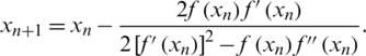
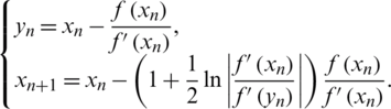
• The modified Halley method (MH) proposed by Said Solaiman et al. [2]:

• The well-known Halley’s method [5], given by:
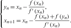
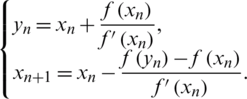
• Potra-Pták (PP) method [23], given by:
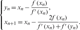
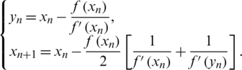
• Weerakon-Fernando (WF) method [24], given by:
• Frontini-Sormani (FS) method [25], given by:
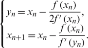
• Homeier method (HM) [26], given by:
• Kou-Wang (KW) method [27], given by:
• Chun method (CM) [28], given by:
The idea of the basins of attraction of f(x) starts by selecting a starting point from a specific region that contains all the roots of f(x). Then we apply the iterative scheme using the selected starting point with specific tolerance and a specific number of iterations considered as a convergence criterion. The iterative scheme will converge to one of the roots in the selected region if it satisfies the convergence criterion, or diverge if it fails. Finally, we color all points which are converging to a specific root using one color, and we use the black color for all points that are failing in satisfying the convergence criterion.
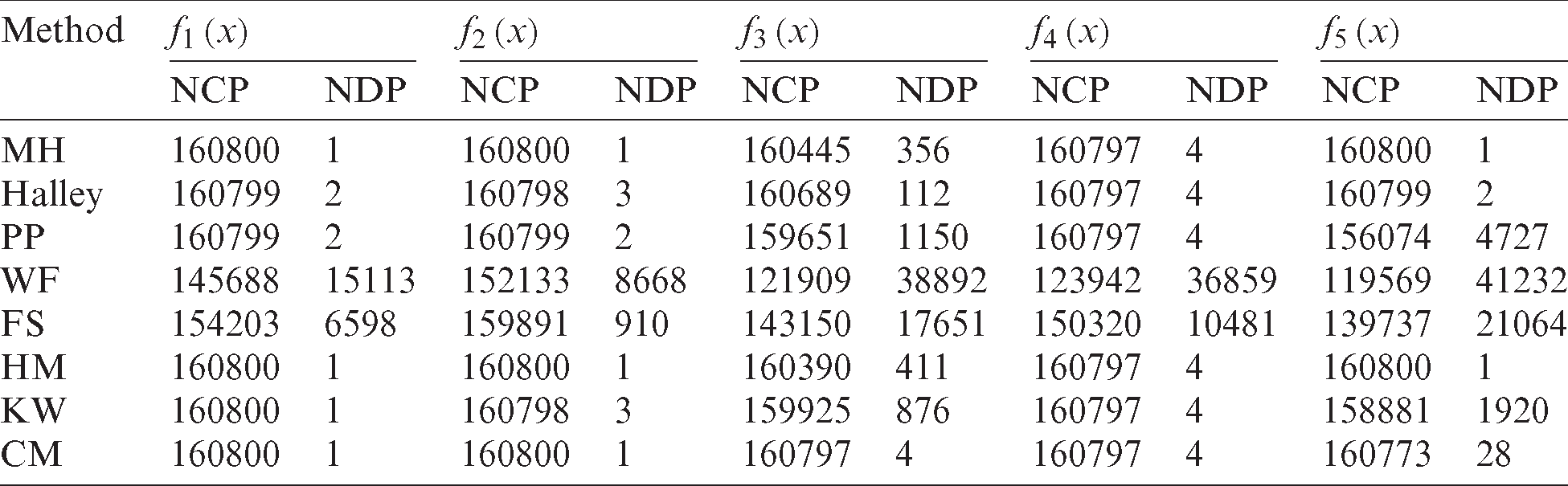
For the purpose of comparison, the CPU time (in sec) needed to obtain the basins of attraction has been computed, see Fig. 6. Moreover, the number of convergent points (NCP) and divergent points (NDP) for each scheme in a selected range have been counted, see Tab. 1. To cover all the zeros of the selected polynomial,  region is centered at the origin. Thus, a
  points in a uniform grid are selected as initial points for the iterative schemes to generate the basins of attraction. Each point in the grid is colored depending on the number of iterations required for convergence and the zero it converges to. The exact roots were assigned as black dots on the graph. If the scheme needs less number of iterations to converge to a specific root, then the region of that roots appears darker. The convergence criterion selected is a tolerance of 10−3 with a maximum of 100 iterations.
Table 1: Number of convergent (NCP) and divergent points (NDP) for 
All calculations have been performed on Intel Core i3-2330M CPU@2.20 GHz with 4 GB RAM, using Microsoft Windows 10, 64 bit based on X64-based processor. Mathematica 9 has been used to produce all graphs and computations.
Example 1 Consider the polynomial 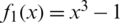 which has roots 1,
  .
.
The basins of attraction for the eight iterative schemes have been showed in Fig. 1. As it can be clearly seen, Halley’s method attains smooth basins of attraction when compared to the others. But, Tab. 1 shows that all iterative schemes except WF and FS have the same area of convergence. From Fig. 6 it is clear that the CPU time needed to attain the basins of attraction is less for MH, Halley, and HM from the remaining schemes. The black areas that appeared in the basins of attraction of WF and FS represent points of divergence.
Figure 1: The basins of attraction for the zeros of f1(x) = x3 −1. The top row from left to right: MH, Halley, and PP. The middle row from left to right: WF, FS, and HM. The bottom row: KW and CM respectively
Example 2 Now, consider the polynomial  which has three simple real roots x = 1,
 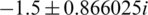 . Looking at Fig. 2 and Tab. 1, one can conclude that WF and FS show a lot of divergent points. The rest of the schemes have better basins of attraction with close CPU time needed to view the graphs as it’s clear from Fig. 6.
Figure 2: The basins of attraction for the zeros of f2(x) = x3+2x2 −3. The top row from left to right: MH, Halley, and PP. The middle row from left to right: WF, FS, and HM. The bottom row: KW and CM, respectively
Example 3 The four roots of unity polynomial  has the roots
  . Even it seems from Fig. 3 that Halley’s method has almost ideal basins of attraction, but we found that it has 112 points of divergent, see Tab. 1. Almost all these 112 points exist on the two main diagonals of the graph. Besides, one can conclude from Tab. 1 that CM is the best for this example as it has the minimum number of points of divergent, even though its basins of attraction has some complexity. So, for this example, we can consider CM as the best regarding the area of the convergence, although it needs little bit more CPU time as it appears from Fig. 6, Halley, MH and HM have also a good area of convergence. The other schemes attain a lot of divergent points.

Figure 3: The basins of attraction for the zeros of f3(x) = x4 −1. The top row from left to right: MH, Halley, and PP. The middle row from left to right: WF, FS, and HM. The bottom row: KW and CM, respectively
Example 4 Next consider  which has the roots
 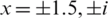 . See Fig. 4 for the basins of attraction of all iterative schemes. In this example all schemes have the same number of convergent points in the selected range, except WF and FS, see Tab. 1. The CPU time needed to display the basins of attraction is less for Halley, MH, and HM from the other schemes, see Fig. 6.
Figure 4: The basins of attraction for the zeros of  . The top row from left to right: MH, Halley, and PP. The middle row from left to right: WF, FS, and HM. The bottom row: KW and CM, respectively
Example 5 Finally, consider  which has the roots
  . From Fig. 5, PP, WF, FS, and KW show clear areas of divergence. These areas resulted from the huge number of divergent points, see Tab. 1. The best scheme in this test problem is MH, HM followed by Halley based on their convergent points in the selected range as it’s clear in Tab. 1. Regarding the required CPU time, Halley is the best followed by HM and MH. See Fig. 6.
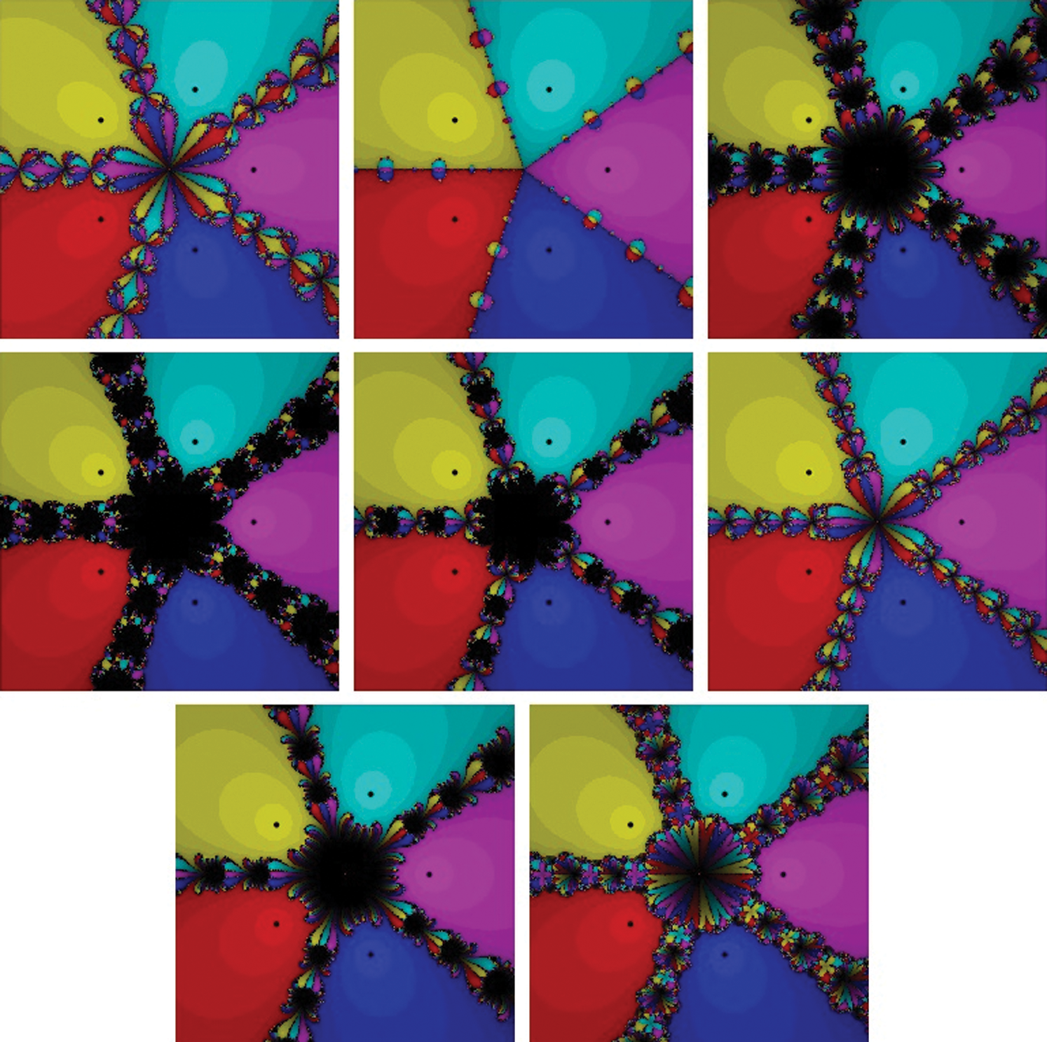
Figure 5: The basins of attraction for the zeros of f5(x) = x5 −1. The top row from left to right: MH, Halley, and PP. The middle row from left to right: WF, FS, and HM. The bottom row: KW and CM respectively
The last set in Fig. 6 shows the average CPU time needed for each scheme when applied to the five test problems. Overall, Halley, MH, and HM need less time to display the basins of attraction of their zeros, followed by CM, PP, KW, FS and WF.

Figure 6: CPU time in seconds
We have compared several iterative schemes for nonlinear equations by visualizing their basins of attraction and finding out the number of convergent and divergent points for the iterative schemes in a selected region. Although all iterative schemes in this work have been selected of equal order of convergence and most of them have an equal number of function evaluations at each iteration, but clear differences have been noted in their behaviors. One can easily note that being an iterative scheme with smooth basins of attraction does not mean that the scheme has a larger area of convergence. In addition, we can conclude that it’s not necessary that a one-step iterative scheme is better than a two-step iterative scheme of the same order. Hence, it is not easy to determine if a specific iterative scheme is better than the other. Finally, even though all the iterative schemes used in this work have the same efficiency index, however, the results show that there are sometimes big differences in their basins of attraction and hence their area of convergence. These results force the need of proposing another index that reflects the real accuracy and efficiency of the iterative schemes.
Funding Statement: We are grateful for the financial support from UKM’s research Grant GUP-2019-033.
Conflicts of Interest: The authors declare that they have no conflicts of interest to report regarding the present study.
1. J. F. Traub. (1964). Iterative Methods for the Solution of Equations. Englewood Cliffs, NJ, USA: Prentice-Hall. [Google Scholar]
2. O. Said Solaiman and I. Hashim. (2019). “Two new efficient sixth order iterative methods for solving nonlinear equations,” Journal of King Saud University—Science, vol. 31, no. 4, pp. 701–705. [Google Scholar]
3. A. Cayley. (1879). “The Newton-Fourier imaginary problem,” American Journal of Mathematics, vol. 2, pp. 97. [Google Scholar]
4. B. Stewart. (2001). “Attractor basins of various root-finding methods,” M.S. thesis, Department of Mathematics, Naval Postgraduate School, Monterey, California, USA. [Google Scholar]
5. E. Halley. (1694). “A new exact and easy method of finding the roots of equations generally and that without any previous reduction,” Philosophical Transactions of the Royal Society, vol. 18, pp. 136–148. [Google Scholar]
6. M. Scott, B. Neta and C. Chun. (2011). “Basin attractors for various methods,” Applied Mathematics and Computation, vol. 218, no. 6, pp. 2584–2599. [Google Scholar]
7. B. Neta, M. Scott and C. Chun. (2012). “Basin attractors for various methods for multiple roots,” Applied Mathematics and Computation, vol. 218, no. 9, pp. 5043–5066. [Google Scholar]
8. N. A. A. Jamaludin, N. M. A. Nik Long, M. Salimi and S. Sharifi. (2019). “Review of some iterative methods for solving nonlinear equations with multiple zeros,” Afrika Matematika, vol. 30, no. 3–4, pp. 355–369. [Google Scholar]
9. S. A. Sariman and I. Hashim. (2020). “New optimal newton-householder methods for solving nonlinear equations and their dynamics,” Computers, Materials & Continua, vol. 65, no. 1, pp. 69–85. [Google Scholar]
10. C. Chun and B. Neta. (2015). “Basins of attraction for several third order methods to find multiple roots of nonlinear equations,” Applied Mathematics and Computation, vol. 268, pp. 129–137. [Google Scholar]
11. B. Neta and C. Chun. (2014). “Basins of attraction for several optimal fourth order methods for multiple roots,” Mathematics and Computers in Simulation, vol. 103, pp. 39–59. [Google Scholar]
12. B. Neta, M. Scott and C. Chun. (2012). “Basins of attraction for several methods to find simple roots of nonlinear equations,” Applied Mathematics and Computation, vol. 218, no. 21, pp. 10548–10556. [Google Scholar]
13. C. Chun and B. Neta. (2016). “The basins of attraction of Murakami’s fifth order family of methods,” Applied Numerical Mathematics, vol. 110, pp. 14–25. [Google Scholar]
14. Y. H. Geum. (2016). “Basins of attraction for optimal third order methods for multiple roots,” Applied Mathematical Sciences, vol. 10, no. 12, pp. 583–590. [Google Scholar]
15. A. Cordero, F. Soleymani, J. R. Torregrosa and S. Shateyi. (2014). “Basins of attraction for various Steffensen-type methods,” Journal of Applied Mathematics, vol. 2014, pp. 17. [Google Scholar]
16. C. Chun and B. Neta. (2017). “Comparative study of eighth-order methods for finding simple roots of nonlinear equations,” Numerical Algorithms, vol. 74, no. 4, pp. 1169–1201. [Google Scholar]
17. E. E. Zotos, M. S. Suraj, A. Mittal and R. Aggarwal. (2018). “Comparing the geometry of the basins of attraction, the speed and the efficiency of several numerical methods,” International Journal of Applied and Computational Mathematics, vol. 4, pp. 105. [Google Scholar]
18. O. Said Solaiman and I. Hashim. (2019). “Efficacy of optimal methods for nonlinear equations with chemical engineering applications,” Mathematical Problems in Engineering, vol. 2019, pp. 11. [Google Scholar]
19. R. Behl, R. González Sarría and A. Magreñán. (2019). “Highly efficient family of iterative methods for solving nonlinear models,” Journal of Computational and Applied Mathematics, vol. 346, pp. 110–132. [Google Scholar]
20. P. Sivakumar, K. Madhu and J. Jayaraman. (2019). “Optimal fourth order methods with its multi-step version for nonlinear equation and their basins of attraction,” SeMA Journal, vol. 76, no. 4, pp. 559–579. [Google Scholar]
21. O. Said Solaiman and I. Hashim. (2021). “An iterative scheme of arbitrary odd order and its basins of attraction for nonlinear systems,” Computers, Materials & Continua, vol. 66, no. 2, pp. 1427–1444. [Google Scholar]
22. S. Amat, S. Busquier and S. Plaza. (2004). “Dynamics of a family of third-order iterative methods that do not require using second derivatives,” Applied Numerical Mathematics, vol. 154, no. 3, pp. 735–746. [Google Scholar]
23. F. Potra and V. Pták. (1984). “Nondiscrete induction and iterative processes. Number,” in Research Notes in Mathematics. Boston: Pitman Advanced Publishing Program. [Google Scholar]
24. S. Weerakoon and T. G. I. Fernando. (2000). “A variant of newton’s method with accelerated third-order convergence,” Applied Mathematics Letters, vol. 13, no. 8, pp. 87–93. [Google Scholar]
25. M. Frontini and E. Sormani. (2003). “Some variant of newton’s method with third-order convergence,” Applied Numerical Mathematics, vol. 140, no. 2–3, pp. 419–426. [Google Scholar]
26. H. H. H. Homeier. (2005). “On Newton-type methods with cubic convergence,” Journal of Computational and Applied Mathematics, vol. 176, no. 2, pp. 425–432. [Google Scholar]
27. J. Kou, Y. Li and X. Wang. (2006). “A modification of newton method with third-order convergence,” Applied Numerical Mathematics, vol. 181, no. 2, pp. 1106–1111. [Google Scholar]
28. C. Chun. (2007). “A method for obtaining iterative formulas of order three,” Applied Mathematics Letters, vol. 20, no. 11, pp. 1103–1109. [Google Scholar]
 | This work is licensed under a Creative Commons Attribution 4.0 International License, which permits unrestricted use, distribution, and reproduction in any medium, provided the original work is properly cited. |