DOI:10.32604/cmc.2021.015099
| Computers, Materials & Continua DOI:10.32604/cmc.2021.015099 | |
| Article |
Prediction of Time Series Empowered with a Novel SREKRLS Algorithm
1School of Computer Science, Minhaj University Lahore, Lahore, 54000, Pakistan
2Prince Sultan University, Riyadh, 11586, Saudi Arabia
3Department of Computer Science, Riphah International University Lahore Campus, Lahore, 54000, Pakistan
4Department of Basic Sciences, Deanship of Common First Year, Jouf University, Sakaka, Aljouf, 72341, Saudi Arabia
5Directorate of IT, The Islamia University of Bahawalpur, Bahawalpur, 63100, Pakistan
6Department of Computer Science, University of Management and Technology, Lahore, 54770, Pakistan
7PUCIT, University of the Punjab, Lahore, 54000, Pakistan
*Corresponding Author: Muhammad Adnan Khan. Email: adnan.khan@riphah.edu.pk
Received: 06 November 2020; Accepted: 03 December 2020
Abstract: For the unforced dynamical non-linear statespace model, a new Q1 and efficient square root extended kernel recursive least square estimation algorithm is developed in this article. The proposed algorithm lends itself towards the parallel implementation as in the FPGA systems. With the help of an ortho-normal triangularization method, which relies on numerically stable givens rotation, matrix inversion causes a computational burden, is reduced. Matrix computation possesses many excellent numerical properties such as singularity, symmetry, skew symmetry, and triangularity is achieved by using this algorithm. The proposed method is validated for the prediction of stationary and non-stationary MackeyGlass Time Series, along with that a component in the x-direction of the Lorenz Times Series is also predicted to illustrate its usefulness. By the learning curves regarding mean square error (MSE) are witnessed for demonstration with prediction performance of the proposed algorithm from where it’s concluded that the proposed algorithm performs better than EKRLS. This new SREKRLS based design positively offers an innovative era towards non-linear systolic arrays, which is efficient in developing very-large-scale integration (VLSI) applications with non-linear input data. Multiple experiments are carried out to validate the reliability, effectiveness, and applicability of the proposed algorithm and with different noise levels compared to the Extended kernel recursive least-squares (EKRLS) algorithm.
Keywords: Kernel methods; square root adaptive filtering; givens rotation; mackey glass time series prediction; recursive least squares; kernel recursive least squares; extended kernel recursive least squares; square root extended kernel recursive least squares algorithm
The Recursive least squares (RLS) algorithm is being studied for the previous two to three decades for solving well known linear signal processing problems such as object tracking, adaptive beamforming, control systems and channel equalization. RLS shows faster convergence than the Least Mean Square Algorithm. However, in non-stationary environments, the performance of the RLS algorithm slightly degrades. Extended RLS and Weighted Extended RLS Algorithm further extend the RLS family that significantly improves its performance in a non-stationary environment. Since the support vector machines have been successful in regression and learning techniques. A further extension to support vector machines is the kernel approach. To generate elegant and efficient nonlinear algorithms, the kernel approach is applied to linear signal processing algorithms such as Least Mean Square, Affine Projection, RLS, Extended RLS and Principal Component Analysis by reworking in the Reproducing Kernel Hilbert Spaces (RKHS) with the framed kernel trick. In recent decades, kernel-based learning algorithms such as vector machine learning, kernel discriminant analysis, kernel principal components analysis, etc., have become widely known for research. In a complicated non-linear environment, these methods illustrate noticeable performance while dealing with regression and classification problems. The motive for the kernel-based approach is to transform content from inputs to feature space and then computing in the feature space through linear learning. The inputs have been transformed into the high dimensional feature space where they are linearly separable, and the linear computations have easily been applied. The famous kernel trick makes an inner product of the inputs linear while working in the high dimensional feature space. Kernel methods such as kernel LMS, kernel RLS, Kernel Affine Projection Algorithm, Extended kernel RLS, and kernel Principal component analysis have gained enormous popularity in the recent past while applied to many complex nonlinear problems [1–4].
To increase the precision and accuracy of the kernel RLS algorithm, an error amending technique for the forecasting of the short-term wind-power system is introduced. This method iteratively collected the data at several intervals and gave a hybrid model for regression in wind power forecasting systems. On the other hand, after carefully selecting the input variables or data window length, this method also captures the characteristics of fluctuation because of the spatial and temporal correlations in wind farms identification error [5].
The restricted window length in the sliding window KRLS algorithm appears to have an inability of handling temporal data points on a larger scale of time. A concept of the reservoir is established that contains a larger number of hidden units. All the units are interconnected sparsely and are viewed as a temporal structure that transforms the time series forecasting history into a particular state space in high dimensional feature space. The KRLS algorithm is used to estimate the relationship between the target and the reservoir state [6].
The prediction of the transition matrix in RKHS is a challenging task. To cope with this issue, an extension in the EKRLS is introduced that constructed the state model in the conventional state space, and the Kalman filter is used to estimate the hidden states. The KRLS Algorithm estimates concealed states in model measurement. This approach shows suitable flexibility in estimating the noise model and allows a linear mapping in RKHS [7].
Kernel adaptive filters use kernel functions that exhibit smoothness, symmetry, and linearity on the entire input domain. The activation function in the neural networks is also a kind of symmetrical kernel function. A flexible kernel expansion-based activation function reduces the overall cost of the system. By using kernels as an activation function in the neural networks helps in approximating the comprehensive mapping specified across a subset on a real line, either non-convex or a convex one [8].
As a network grows with the incoming data samples, the overall computation time and memory time increases. A compact and accurate method of restricting network’s size can accelerate the learning time and computational burden in the kernel adaptive filtering. A least important data sample is removed from the dictionary and ordering the remaining data in centers by the value of their importance. This pruning technique to KRLS dramatically improves the convergence time of KRLS [9].
Linear LMS is used for training the weights in the Cerebellar Model Articulated Neural (CMAC) Network in an online manner [10]. CMAC method is a fast converging method, and typically only one epoch is required, so there is no issue of selecting a suitable learning rate. The use of the RLS algorithm in CMAC for weight updating is computationally inefficient [11–14]. Kernel methods for CMAC, on the other hand, does have a computational burden, but the memory requirement and modeling capabilities are somehow improved [15,16].
This research work presents a novelty of the square root EKRLS algorithm with a spontaneous dynamic model’s prediction for chaotic stationary and non-stationary time series. The square root version of EKRLS converges fast as compared to the EKRLS. The computational burden is also lowered because of the givens rotation that gives excellent online numerical stability. At each time step, the new patterns are added in the data window of the given’s rotation in the triangular form, and the rotations are performed with sines and cosines that avoid inverse at each iteration. The usefulness of the proposed algorithm is checked on the estimation for stationary and non-stationary cases of the chaotic and non-linear Mackey Glass time series prediction.
The structure of the given paper is constructed with six sections. In, Section 2 details about the Extended RLS algorithm are presented. Section 3 carries a brief introduction of kernels and EKRLS. A unique unforced dynamical model of the proposed SREKRLS algorithm has discoursed in Section 4. For simplicity, all deviations and formulation of the algorithm are performed with the help of real variables. Section 5 holds the result of the simulation and discussion under the proposed framework. Conclusion and future directions are presented in Section 6.
When describing sequential approximation, a generic linear state-space model is given as:


Eq. (1) represents the space model, and Eq. (2) represents an observation model. Here  ,
,  and
and  represents the state transition matrix,state noise
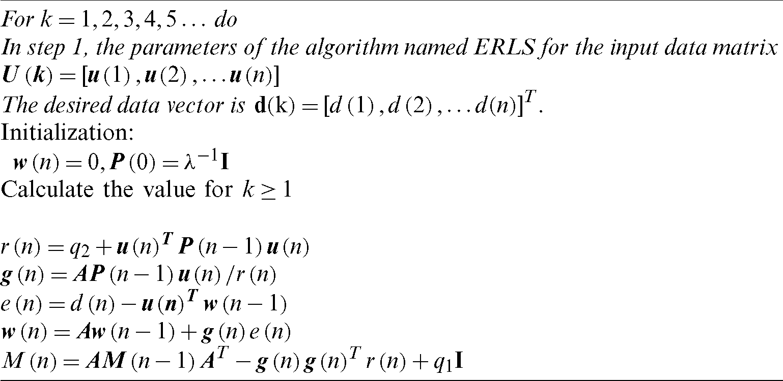
  and even the process noise or observation. The state model is commonly referred to as the process equation, while the observation model is referred to as the measurement equation. Either the noises are white as well as the Gaussian distribution. Tab. 1 shown Algorithm 2, which contains a summary of the Extended recursive least square algorithm (ERLS).
3 Introduction to Kernel Methods and EKRLS Algorithm
This section is about the detailed description of positive definite kernels, feature space, or reproducing kernel Hilbert space, then the EKRLS algorithm along-with brief short details of the algorithm.
The intended theme of using kernel functions is carrying out the transformation of points  of input data to
  a feature space as
  . To discover the presence of linear relationships in data, several different methods can be applied in feature space [2]. Symmetric, continuous, and positive definite property is maintained by the kernel method.
  , X: input domain, a subset of
  . The Gaussian kernel function is perhaps the most widely used kernel function:-

Here, the kernel’s width is represented by  . An adaptive algorithm is aided by kernel function for the manipulation of converted input data in feature space. Kernel function allows the adaptive algorithm to manage transformed inputs in feature space not know co-ordinates of data in a given space. The kernel function maintains the property of symmetry and convexity throughout the domain.
As per mercer’s principle [1,2] every kernel mechanism  masks or transforms the input data in high dimensional feature space (reproducing kernel Hilbert space) [8] and generally calculated through inner products, provided as:

Thus mapping/projection is being performed as  . This method is also known as the famous kernel trick. The specified scheme is recycled to develop an algorithm named kernel filtering.
3.2 Extended Kernel Recursive Least Squares Algorithm
Triggering through particular un-forced dynamical non-linear state-space model state model is given in Eq. (5).

The measurement model is given in Eq. (6).

With the mean of zero, the measurement noise is white as well as no process noise due to a spontaneous dynamic model. When considering the model as mentioned above, recurrent ERSL equations are written as:

Eq. (7) is the difference equation named Riccati in feature space. By keeping in view, the dimensions of this equation. This equation will be Decomposed and adjusted in matrix form for further computations through the given’s notation.
In Fig. 1, the primary cell structure is described in the given’s rotation using high dimension feature space. The transition matrix will be dependent on the value of lambda.

Figure 1: Cell structure of the square root elements
Fig. 2 described the complete architecture of the given rotation works in RKHS. In the first quadrant, the input is transformed in the high dimensional feature space using a positive definite Gaussian kernel function. Then the inverse of the Riccati difference equation is computed by decomposing the  in the triangular form.

Figure 2: Architecture of the given’s rotation in the feature space
4 Proposed Square Root Extended Kernel Recursive Least Squares Algorithm
To acquire KRLS rotation-based characteristic for the unforced dynamic model, we first totally disregard the term  because
  reduces as well as organizes the essential terms in the form of a matrix consisting of the critical terms noted as:
1. A 
2. A 
3. A vector 
4. An 
Given four terms, it carries all the information regarding Riccati difference Eq. (7). By keeping an eye on the dimensionality of these terms, we can arrange the terms described above in the form of a matrix, and the combined form of these terms will be written as given below:-

Its factored form yields.

We interpreted the equation’s RHS (8) as one matrix’ product and its transposed term. Application of this interpretation & matrix decomposition Lemma, we then set the Eq. (5) and calculate the unspecified or unclear as in Eq. (9).

Non-zero block elements of the matrix call it matrix B is made up of scalar b11(n), vector term  and matrix
  that forms as a result of unitary rotation
  . To determine the missing or unknown elements in Eq. (7), take a square on both sides of Eq. (9).

By identifying point which  is a unit matrix and hence, it is resultant
  is equivalent to unity. The remaining concepts are worded as follows:


When fulfilling the above mentioned in Eqs. (10)–(13).


The concept  is the one-half power variance. The second equation accounts for the gain together with the term of variance. The Cholesky state-error correlation factor matrix is given for the third term.

The  and 0 elements in the pre-array induce 2 variables to be created: r(n) variance and
  gain. Both these variables come mainly from the division and squaring term of
  . The series of equations Eq. (14) through Eq. (16) gives a specific description of the extended kernel Square root RLS and explicitly provides us with definitions of EKRLS parameters. However, irrespective of this, the actual practice of a rotation matrix is
  which is a unit matrix excluding for 4 points wherever the pairs of the poles k and l overlap. The pairs of column’s rows k and l are symbolized as rows k and,
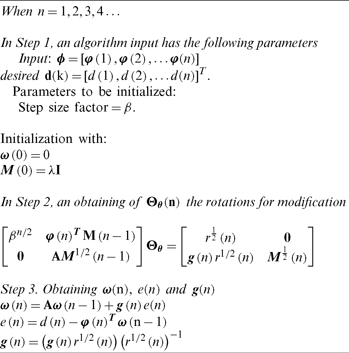
  respectively. A complete summary of an algorithm is specified in Tab. 2, articulates the calculation from pre-array to pasture.
Table 2: SREKRLS (spontaneous dynamical model) algorithm
In this part of a given paper, the findings of the prediction of Mackey Glass Time Series and the x-component of the 3-dimensional prediction of the Lorenz time series are discussed with the aid of the suggested algorithm.
5.1 Prediction of Mackey Glass Time Series (PMGTS)
To estimate MGTS, we found both stationary and non-stationary time series in this experiment. The Mackey Glass Time Series is created using the delay differential equation given below:

With  ,
,  and
and  . So, we obtain a series x(t) for
 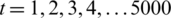 by the delay as mentioned above differential equation. The series is received by the continuous curve of x(t) with the time of a one-second interval. The cost function of the time series projections/predictions is provided here as
  , here,
  ,
,  and
and  are represents the weights that have been trained and samples for training, respectively.
  ,
,  denote weights that are trained and
  denote samples that are utilized for testing.
In this experiment, the filter’s order is taken as 10, i.e.,  , for the prediction of the current one
  previous 10 sample points are used as input. Three thousand (3000) sampling points have been used for training purposes, while the next 250 sample points are absorbed with the proposed EKRLS algorithm for testing. Training with 1501–4500 sample points on the stationary sequence for the output analysis of the proposed algorithm is performed, while 4600–4850 sample points are used to evaluate the proposed algorithm. During the training step, weights are modified and tested using all these modified weights; learning curves are produced to evaluate the proposed algorithm through MSE (mean square error). Noise is applied to time series with multiple variances for further validation of the proposed algorithm’s output. Five hundred (500) Monte Carlo simulations are run for algorithmic weights modification, and these modified weights are used for the sample prediction. To produce results, zero-mean additive noise with a variance of 0.09 is applied to series; see Fig. 3.

Figure 3: Mean square error curves with stationary MGTSP for EKRLS and SREKRLS while noise variance 
The algorithm parameters used are set as EKRLS  with
with 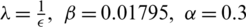 and Gaussian kernel with a width of 0.2), and the offered SREKRLS
  with
with  and Gaussian kernel with a width of 0.3).
AWG noise of variance (0.07) is applied to the unique series, and the estimated output of the suggested algorithm is enhanced by 0.01 dB. The noise level for the proposed algorithm is increased by a variance of 0.20 to confirm the output and outcomes further; enhancement of 0.07 dB is shown with the EKRLS algorithm. From tests, it’s derived that the proposed algorithm shows more noise robustness.
The curves present in Fig. 4 depict the progression of 0.04 dB through the noise of variance of 0.2 and 0.05 dB progression if the noise of variance of 0.1 is applied; data present in Tab. 3 shows mean square error with different noise variances for EKRLS and SREKRLS.

Figure 4: MSE curve of EKRLS and SREKRLS for stationary Mackey Glass Time series Prediction with noise variance 0.1
Table 3: Mean square error with stationary MGTSP at different noise variance
See Tab. 3 for a comparative analysis of the proposed algorithm with EKRLS at different noise variance levels. It is noted that SREKRLS gives more attractive results in terms of mean square error as comparedto EKRLS. It’s also observed that the proposed SREKRLS gives more accurate results with high noise variance.
For more examination and validation of the proposed algorithm’s behavior in comparison with EKRLS, a non-stationary series with the addition of a sinusoidal ( , f = 1/5000) with an amplitude of 0.3 having an occurrence of five thousand (5000) samples/second is summed up with original MGTSP. The same factors and samples are used as in stationary series.
Figs. 5–8 show that MSE curves when noise variance is set as 0.09, 0.07, 0.2, and 0.1, respectively.

Figure 5: Mean square error with non-stationary MGTSP for EKRLS and SREKRLS while noise variance 

Figure 6: Mean square error with non-stationary MGTSP for EKRLS and SREKRLS while noise variance 

Figure 7: Mean square error for x-component of LTSP of EKRLS and SREKRLS while noise variance is absent

Figure 8: Mean square error for x-component of LTSP of EKRLS and SREKRLS while noise variance 
Tab. 4 provides insight into the mean square error values for different values of noise variance (NV) with non-stationary MGTSP for both EKRLS and SREKRLS.
Table 4: Mean square error with non-stationary MGTSP at different noise variance

5.2 Lorenz’ Time Series Prediction
The Lorenz series is a non-linear, 3D, and deterministic equation. It is represented as a sequence of fractional differential equations provided under:


Lorenz’ unpredictable conduct on the parameters,  ,
,  and
and  . With the help of a first-order approximation procedure including a sample time of 0.001 s with some the initial conditions are defined as
  and
and  . This type of series is a three-dimensional (3D) Lorenz series. Thus finding the component named as x of LTS and derive 5000 training incidences, i.e., 1500–4500 for the preparation of training the suggested algorithm and its corresponding part, while the rest of the 300 samples are utilized as a testing set. In terms of mean square error, learning curves in the absence of noise are shown in Fig. 8. To predict the current one, the sequence of the filter is designated as three (3). The algorithm parameters can be optimized as EKRLS:
  with
with  (and Gaussian kernel with a width of 0.2, and the proposed SREKRLS
  with
with  and Gaussian kernel with a width of 0.4).
In Fig. 8 Proposed algorithm’s performance is evaluated without adding noise; performance improvement is recorded of 0.02 dB as compared to EKRLS.
For further investigation in performance, noise variance of 0.09 is added in Lorenz Series’ x-component, and performance is observed see Fig. 8.
Performance results produced by the proposed algorithm compared to EKRLS are displayed in Tab. 5. When noise is present or absent, conditions are applied to series generated to the X-Component of LTSP with different noise variances.
Table 5: Mean square error for x-component of LTSP of EKRLS and SREKRLS

The proposed algorithm offers an enhanced square root algorithm called Extended Kernel Recursive Least Square (EKRTS). The EKRLS algorithm topic is also presented with reasonable discussion. One version of the stationary and non-stationary Mackey Glass Time Series prediction is seen at various noise levels. By the learning curves regarding mean square error (MSE) are witnessed for demonstration with prediction performance of the proposed algorithm from where it’s concluded that the proposed algorithm performs better than EKRLS. For further testing, the validity of the proposed algorithm, LTSP’s x-component is also predicted. This new SREKRLS based design positively offers an innovative era towards non-linear systolic arrays, which is efficient in developing very-large-scale integration (VLSI) applications with non-linear input data.
Acknowledgement: Thanks to our families & colleagues, who supported us morally.
Funding Statement: This work is funded by Prince Sultan University, Riyadh, Saudi Arabia.
Conflicts of Interest: The authors declare that they have no conflicts of interest to report regarding the present study.
1. S. Haykin. (2010). Support vector machines. In: Neural Networks and Learning Machines. ed. India: Pearson Education India, pp. 268–313. [Google Scholar]
2. W. Liu, J. C. Principe and S. Haykin. (2011). “Kernel least-mean-square algorithm,” Kernel Adaptive Filtering: A Comprehensive Introduction, vol. 57, pp. 27–68. [Google Scholar]
3. W. D. Parreira, J. C. M. Bermudez, C. Richard and J. Y. Tourneret. (2012). “Stochastic behaviour analysis of the Gaussian kernel least-mean-square algorithm,” IEEE Transactions on Signal Processing, vol. 60, no. 5, pp. 2208–2222. [Google Scholar]
4. K. Li and J. C. Principe. (2017). “Transfer learning in adaptive filters: The nearest instance centroid-estimation kernel least-mean-square algorithm,” IEEE Transactions on Signal Processing, vol. 65, no. 24, pp. 6520–6535. [Google Scholar]
5. M. Xu, Z. Lu, Y. Qiao and Y. Min. (2017). “Modelling of wind power forecasting errors based on kernel recursive least-squares method,” Journal of Modern Power Systems and Clean Energy, vol. 5, no. 5, pp. 735–745. [Google Scholar]
6. H. Zhou, J. Huang, F. Lu, J. Thiyagalingam and T. Kirubarajan. (2018). “Echo state kernel recursive least squares algorithm for machine condition prediction,” Mechanical Systems and Signal Processing, vol. 111, pp. 68–86. [Google Scholar]
7. S. Scardapane, S. Van Vaerenbergh, S. Totaro and A. Uncini. (2019). “Kafnets: Kernel-based non-parametric activation functions for neural networks,” Neural Networks, vol. 110, pp. 19–32. [Google Scholar]
8. P. Zhu, B. Chen and J. C. Príncipe. (2012). “A novel extended kernel recursive least squares algorithm,” Neural Networks, vol. 32, pp. 349–357. [Google Scholar]
9. H. Zhou, J. Huang and F. Lu. (2018). “Parsimonious kernel recursive least squares algorithm for aero-engine health diagnosis,” IEEE Access, vol. 6, pp. 74687–74698. [Google Scholar]
10. C. Laufer, N. Patel and G. Coghill. (2014). “The kernel recursive least squares cmac with vector eligibility,” Neural Processing Letters, vol. 39, no. 3, pp. 269–284. [Google Scholar]
11. M. Han, S. Zhang, M. Xu, T. Qiu and N. Wang. (2018). “Multivariate chaotic time series online prediction based on improved kernel recursive least squares algorithm,” IEEE Transactions on Cybernetics, vol. 49, no. 4, pp. 1160–1172. [Google Scholar]
12. H. Cheng. (2013). “The fuzzy CMAC based on RLS algorithm,” Applied Mechanics and Materials, vol. 432, pp. 478–482. [Google Scholar]
13. C. W. Laufer and G. Coghill. (2013). “Kernel recursive least squares for the CMAC neural network,” International Journal of Computer Theory and Engineering, vol. 5, no. 3, pp. 454–459. [Google Scholar]
14. M. Han, S. Zhang, M. Xu, T. Qiu and N. Wang. (2018). “Multivariate chaotic time series online prediction based on improved kernel recursive least squares algorithm,” IEEE Transactions on Cybernetics, vol. 49, no. 4, pp. 1160–1172. [Google Scholar]
15. C. W. Laufer and G. Coghill. (2013). “Kernel recursive least squares for the CMAC neural network,” International Journal of Computer Theory and Engineering, vol. 5, no. 3, pp. 454–463. [Google Scholar]
16. F. J. Lin, I. F. Sun, K. J. Yang and J. K. Chang. (2016). “Recurrent fuzzy neural cerebellar model articulation network fault-tolerant control of six-phase permanent magnet synchronous motor position servo drive,” IEEE Transactions on Fuzzy Systems, vol. 24, no. 1, pp. 153–167. [Google Scholar]
 | This work is licensed under a Creative Commons Attribution 4.0 International License, which permits unrestricted use, distribution, and reproduction in any medium, provided the original work is properly cited. |