DOI:10.32604/cmc.2021.015089
| Computers, Materials & Continua DOI:10.32604/cmc.2021.015089 | |
| Article |
Modeling Liver Cancer and Leukemia Data Using Arcsine-Gaussian Distribution
1Department of Statistics, Faculty of Science, King Abdulaziz University, Jeddah, 21589, Saudi Arabia
2Department of Statistics, Faculty of Commerce, Zagazig University, Zagazig, 44511, Egypt
3Department of Statistics, Mathematics and Insurance, Benha University, Benha, 13511, Egypt
*Corresponding Author: Ahmed Z. Afify. Email: ahmed.afify@fcom.bu.edu.eg
Received: 06 November 2020; Accepted: 12 December 2020
Abstract: The main objective of this paper is to discuss a general family of distributions generated from the symmetrical arcsine distribution. The considered family includes various asymmetrical and symmetrical probability distributions as special cases. A particular case of a symmetrical probability distribution from this family is the Arcsine–Gaussian distribution. Key statistical properties of this distribution including quantile, mean residual life, order statistics and moments are derived. The Arcsine–Gaussian parameters are estimated using two classical estimation methods called moments and maximum likelihood methods. A simulation study which provides asymptotic distribution of all considered point estimators, 90% and 95% asymptotic confidence intervals are performed to examine the estimation efficiency of the considered methods numerically. The simulation results show that both biases and variances of the estimators tend to zero as the sample size increases, i.e., the estimators are asymptotically consistent. Also, when the sample size increases the coverage probabilities of the confidence intervals increase to the nominal levels, while the corresponding length decrease and approach zero. Two real data sets from the medicine filed are used to illustrate the flexibility of the Arcsine–Gaussian distribution as compared with the normal, logistic, and Cauchy models. The proposed distribution is very versatile to fit real applications and can be used as a good alternative to the traditional gaussian distribution.
Keywords: Liver cancer data; leukemia data; normal distribution; moments estimation; maximum likelihood estimation
In the last two decades, several methods are proposed to generate continuous distributions. Many of these methods are discussed in [1]. The methodologies of these methods depend on generating new distributions by adding parameters to an existing distribution or combining existing distributions, see for more details [2,3]. The beta distribution is an important model for the analysis of proportions which are common in many fields of science such as toxicology [4]. A particular case of the beta distribution is the symmetric arcsine distribution which is a beta distribution with both shape parameters equal to half. In the field of stochastic process, the arcsine distribution is associated with the arcsine laws of random walks and Brownian motion [5]. For more comperhansive details about the beta distribution, see [4,6].
A continuous random variable X is said to follows the standard arcsine distribution if its cumulative density function (CDF) is given by:

Now, notice that the x term in the right hand side of (1) is actually the CDF of a standard uniform distribution. Hence, by simply replacing this term with another CDF of any continuous probability distribution; say,  , then one can obtain an extended arcsine distribution with the following CDF:

Clearly, this extension of the arcsine distribution can generate lifetime distributions and elliptically contoured distributions (i.e., symmetrical distributions in  (by simply replacing
  with the corresponding CDF of the considered probability distribution. For more details about different kinds of univariate continuous distributions, see [7]. In statistical literature, researchers have proposed generalizations and extensions for many continuous probability distributions. Obviously, when modeling real data, obtaining a generalization or an extension for a model of interest provides a more flexible version of the model which may fit the data more appropriately. For instance, the exponential distribution is extensively considered in reliability data with a constant failure rate. In practice, however, several reliability data may have monotonic failure (hazard) rates. Thus, a well-known generalization for the exponential distribution; namely, the Weibull distribution, is alternatively considered. Although constant and monotonic failure rates might be encountered in reality, many real-life data have non-monotonic failure rates. Consequently, researchers have considered various generalization for the Weibull distribution, see the concise article by [8] in this connection.
Recently, several generalizations of the normal distribution have been developed. For example, the beta-normal distribution [9], generalized normal distribution [10], skew-normal distribution [11], and truncated normal distribution [12].
This study considers the extension of the arcsine distribution based on a gaussian kernel which is henceforth called the arcsine-gaussian (AG) distribution. The motivations to propose the AG distribution are: (1) To develop various shapes for the density and hazard rate function of the distribution. (2) To increase the flexibility of the classical gaussian distribution in modelling different real life applications. (3) To increase the flexibility of the traditional gaussian distribution properties like mean, variance, skewness and kurtosis. (4) The analysis of two real data sets proved that the AG distribution provides a better fit than the traditional gaussian distribution and some of its competitive models. Although the idea of this paper is not new since the AG distribution is a special case of the beta-normal distribution [9], the novelty of this study lies in the fact that, to the best of the author’s knowledge, no previous research has been conducted on this probability distribution although the importance and popularity of the gaussian distribution in modeling many real-life applications. The remaining sections of this article are organized as follows. Sections 2 and 3 discuss the distributional and statistical properties of the AG distribution, respectively. In Section 4, estimators are derived for the model parameters and their finite-sample efficiencies are numerically examined using Monte Carlo simulations in Section 5. Two real life data sets are analyzed in Section 5 to illustrate that the AG distribution is a suitable fit for the two data under analysis, comparing with some well-known distributions. Finally, the paper is concluded in Section 7.
2 Distributional Properties of the AG Distribution
In this section, the distributional properties of the AG distribution are discussed.
2.1 The CDF and the Survival Function
By replacing  in expression (2) by CDF of the gaussian distribution, denoted by
  , one can say that a random variable X follows the AG distribution with location parameter
  and a non-negative scale parameter
  0 (i.e.,
  ) if the CDF and the survival function (SF) have the following forms, respectively:

and

Clearly, the AG distribution is a location-scale model; i.e., if  , then
  .
.
It is well-known that the quantile function finds the value X such that
for a probability 0 < u < 1. Fortunately, the AG distribution has an advantage that the corresponding CDF has an explicit form and is a strictly increasing function. Consequently, the qunatile function is straightforwardly defined as follows:

where  is the the quantile function of the standard gaussian distribution. Note that one can verify that the median of the AG distribution is equal to
  by setting u = 0.5 in expression (5).
2.3 The Probability Density Function
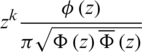
By differentiating both part of (3) with respect to x, one can show that the probability density function (PDF) of the AG function with location parameter  and a scale parameter
  is given by:

where  and
and  are the PDF, CDF, and SF of the standard gaussian (normal) distribution, respectively. Clearly, the distribution is symmetric and this fact is proven in the following lemma.
Lemma 1  is symmetric about its location parameter
  .
.
Proof. A continuous probability distribution is said to be symmetric about its location parameter  if and only
  for all
  . Clearly,
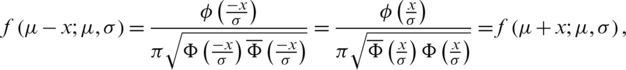
since  and
and  .
.
Note that additional statistical proprieties are to be addressed in the following section. Fig. 1 shows some possible shapes of the AG density for various values of  and
and  .
.
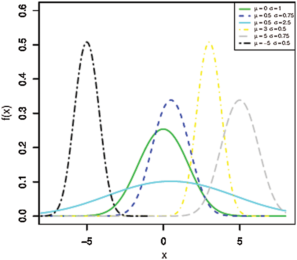
Figure 1: The PDFs of the AG distribution for different values of  and
and 
The AG distributional not only is symmetric like the Gaussian distribution, but also inherits the behavior of its hazard function (HF). That is, the HF is increasing, see Fig. 2. The HF of the AG function with location parameter  and a scale parameter
  is given by:

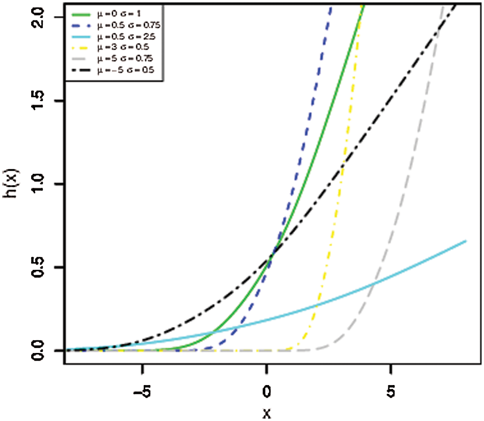
Figure 2: The HRFs of the AG distribution for different values of  and
and 
A probability distribution with an increasing HF is suitable to model lifetime data observed due to wear-out of lifeless objects or aging of living entities. Mathematically speaking, this can be proven as follows.
Theorem 1  has an increasing hazard rate.
Proof. Without loss of generality, consider the standard AG distribution. Notice that expression (7) can be rewritten as:
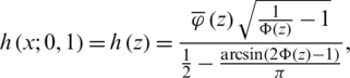
where  is the HF of the standard gaussian distribution. Taking the natural logarithm on both side yields:

The term  is proven to be increasing by [13], while the third is the cumulative HF of the AG distribution which is increasing be definition. Notice that:
As previously mentioned,  is increasing and so does
  since
since  is increasing,
  is decreasing, and
  is increasing. Because the second term is increasing for all values of z, then
  is increasing due to the fact that all of its components are increasing by the definition of increasing functions.
According to Theorem 1, the HF of the AG model is increasing function in its parameters as displayed graphically in Fig. 2, for various values of  and
and  .
.
In reliability analysis, the mean residual life (MRL) is an important characteristic of a lifetime model. Let  denotes the MRL of the AG distribution; then:

where  and
and  are the SF and the PDF of the probability distribution of interest. Notice that expression (8) can be rewritten in terms of the HF as follows:

where  is the HF of the considered distribution; see [14,15] in this connection. Hence, form expression (9), one can easily infer that the MRL in the case of the AG distribution has an opposite behavior to that of the HF, i.e., it is decreasing
  . This observation is asserted in Fig. 3.
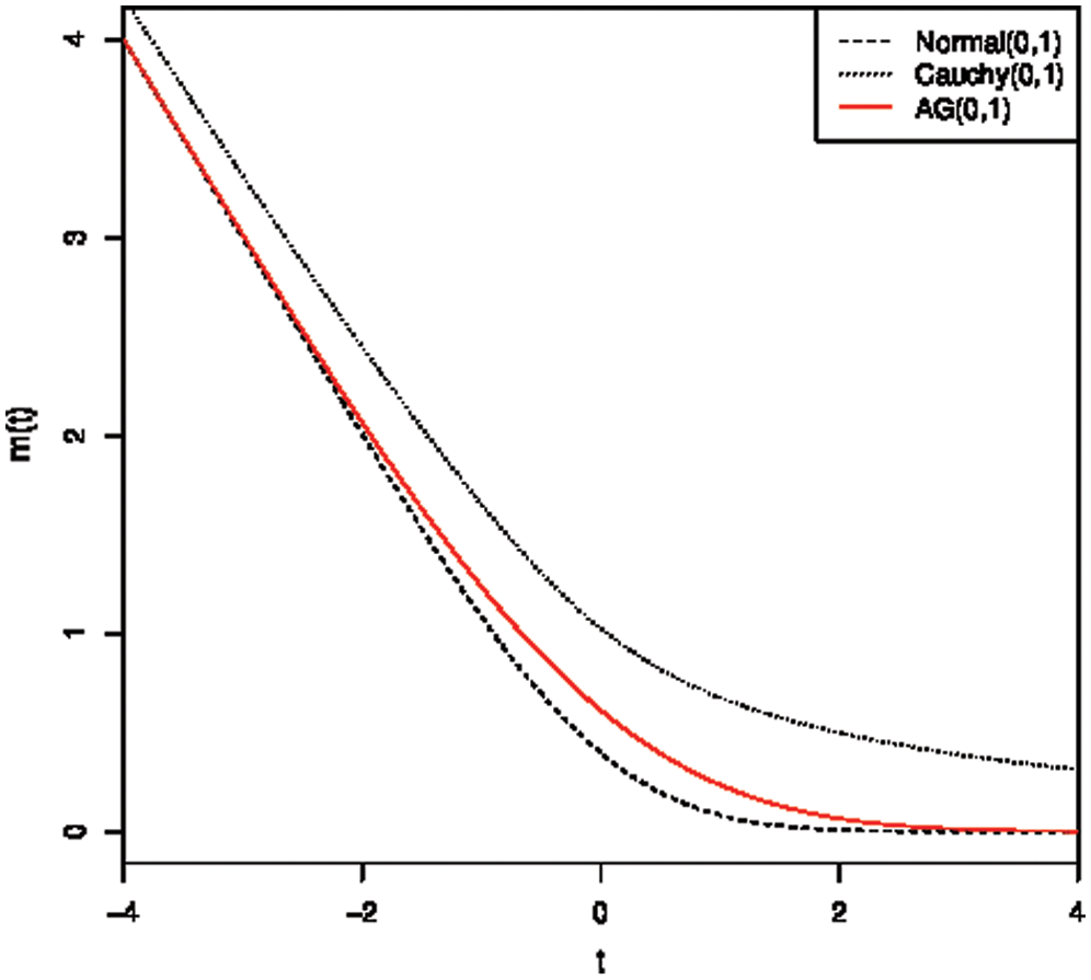
Figure 3: The MRL of the AG, normal and Chancy distributions with  and
and 
In this section, the PDF of the r-th order statistics is derived. Let  be the order statistics for a random sample
  of size n from the AG distribution. It is known that the PDF of the r-th takes the form
where  and
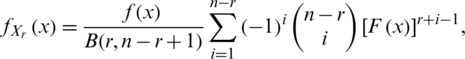
and  are the CDF and PDF of the AG distribution. From (3) and (6), the PDF of the r-th order statistics of the AG distribution is given by

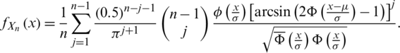
Particularly, PDF of the first and last order statistics can be derived directly from the last equation as follow
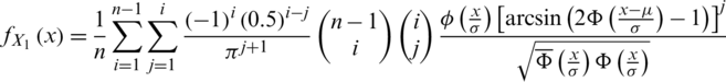
and
3 Statistical Properties of the AG Distribution
This section presents several statistical properties of the AG distribution which are obtained from the following lemma and theorem.
Lemma 2
1. The quantile function of the standard normal distribution; namely,  , is increasing for all
  .
.
2. If  , then
  for all
  and
and  .
.
Proof.
1. If  , then
  . Differentiating both sides of the latter equation with respect to q yields:
Hence,  is an increasing function for all
  .
.
2. Recall that  is increasing and let
  ; thus,
  since
since  . Hence, the proof is completed by taking the expected value on all sides of the inequality and making use of the properties of the expectation operator (see [16] in this connection), and by taking the limit
  .
.
Theorem 2 If  , then the kth moment exists for
such that
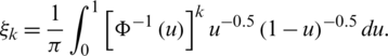
Proof. For any value of k, it is clear that:

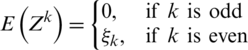
Hence, E(Xk) is finite according to Lemma 2. However, if k is a positive odd integer (i.e.,  ), then the term
is clearly an odd function since the AG distribution is symmetric according to Lemma 1. Hence, E(Zk) = 0 for  .
.
By making use of Theorem 2 and the the fact that the AG distribution is a location-scale and a symmetric family of distributions, its properties are straightforwardly obtained as follows.
Corollary 1 If  , then the measures of center tendency; namely, the mean, median, and the mode are equal to
  .
.
Corollary 2 If  , then the second, third, and forth moments of X are given by:

respectively.
Corollary 3 If  , then the variance is given by:

Corollary 4 Let  (
( ) denote the coefficient of skewness (kurtosis), if
  ,
,  , while
  .86158.
It is to be noted that the above corollaries agree with the result of [9].
In this section, two methods are considered to estimate the parameters of the AG distribution; namely, the method of moments and the maximum likelihood method.
Suppose that  represent a random sample from the AG distribution with location parameter
  and a scale parameter
  . By employing the method of moments, the corresponding moments estimator (ME) for
  ; say,
  , is the sample mean (i.e.,
  ), while the ME for
  ; say,
  , is given by:

Notice that one can obtain a Monte Carlo moments estimator (MCME) for  based on expression (11) using Monte Carlo integration (MCI). To improve the approximation, the variance is reduced using antithetic variates. For more information about the latter method and MCI, see [17]. The MCME estimator of
  ; say,
  , is calculated by approximating the term
  in (11) as follows:
1. Generate a random sample  from
from  .
.
2. 
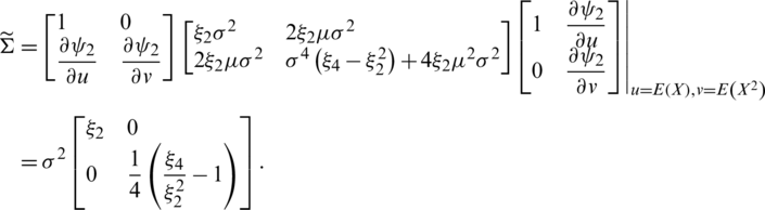
Theorem 3 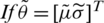 , then the asymptotic joint sampling distribution
  is a bivariate normal (BN) distribution with mean vector
  and variance–covariance matrix
  , i.e., 1

such that  is the zero vector and
Proof. Recall that  represent a random sample (i.e., independent and identically distributed random variables) from the
  . Suppose that:
By the strong law of large numbers, M1 and M2 converge almost surely to E(X) and E(X2), respectively. Furthermore, by the central limit theorem, both M1 and M2 are asymptotically normally distributed. Also, any linear combination of M1 and M2; say, c1M1 +c2M2, is asymptotically normally distributed for all c1 and c2. Accordingly,

where
such that

and

by making use of the corollaries in the previous section. Now, the aim is to find the asymptotic joint sampling distribution of

such that  and
and 
Notice that:

Hence, by making use of Taylor series expansion, one can easily verify that
where
4.2 Maximum Likelihood Estimators
Recall the PDF of the AG distribution which was given by expression (6). Also, suppose that  are the observed order statistics. The likelihood function based on
  is then
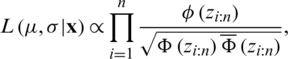
such that  . Accordingly, the log-likelihood function is as follows:

where  . From (13), the likelihood (normal) equations for
  and
and  are, respectively:

and

such that  and
and  are the HF and the reversed HF of the standard gaussian distribution, respectivly. The latter function is decreasing for all real numbers and this can be proven using a methodology simiar to that of [13].
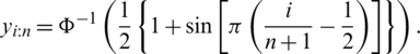
Clearly, the values of the maximum likelihood estimators (MLEs) need to determined numerically. Nevertheless, by following a similar approach as in [13], one can derive the following approximated MLEs for both  and
and  based on the observed order statistics
  :
:
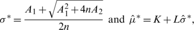
such that
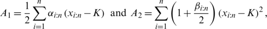
while
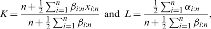
where
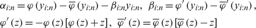
and
Unfortunately, it is not easy to derive the exact distributions for both the MLEs and their approximated counterparts. However, one may can derive asymptotic confidence intervals for the model parameters under some regularity condition. For more information about the asymptotic properties of the MLEs, see [16]. Now, according to the latter reference, as  , then:
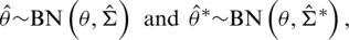
such that  ,
,
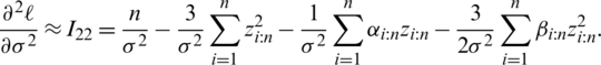
where 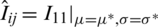 for i, j = 1, 2, such that
and
To compare the estimation methods in terms of efficiency, extensive MC simulations are carried out. The outcomes of an MC simulation study are reported in this section. Without loss of any generality, the standard AG distribution is considered, while the sample sizes of interest are n = 10(10)100. The numerical results of this study were determined from 10,000 MC simulation runs. This number of simulations gives the accuracy in the order  see, [18]; thus, all numerical outcomes for this study are reported up to three decimal digits.
Tab. 1 presents the outcomes associated with the estimators of  ; namely, the ME (
 ), the AMLE (
 ), and the MLE
  . On the other hand, Tab. 2 summarizes the simulation results of the estimators of
  ; namely, the MCME (
 ), the ME (
 ), the AMLE (
 ), and the MLE
  . By making use of the asymptotic distribution of all considered point estimators, 90% and 95% asymptotic confidence interval are obtained and are evaluated according to their observed coverage probabilities and lengths. Interestingly, all estimators had similar performance indicators. Furthermore, the simulated variance of the estimators and their counterparts which were calculated based on the variance-covariance matrix (VCM) of the asymptotic sampling joint distributions were quite close.
Table 1: Bias and variance for the estimators of  alongside the observed coverage probability (CPr) and length (L) of 90% and 95% confidence intervals (CIs)
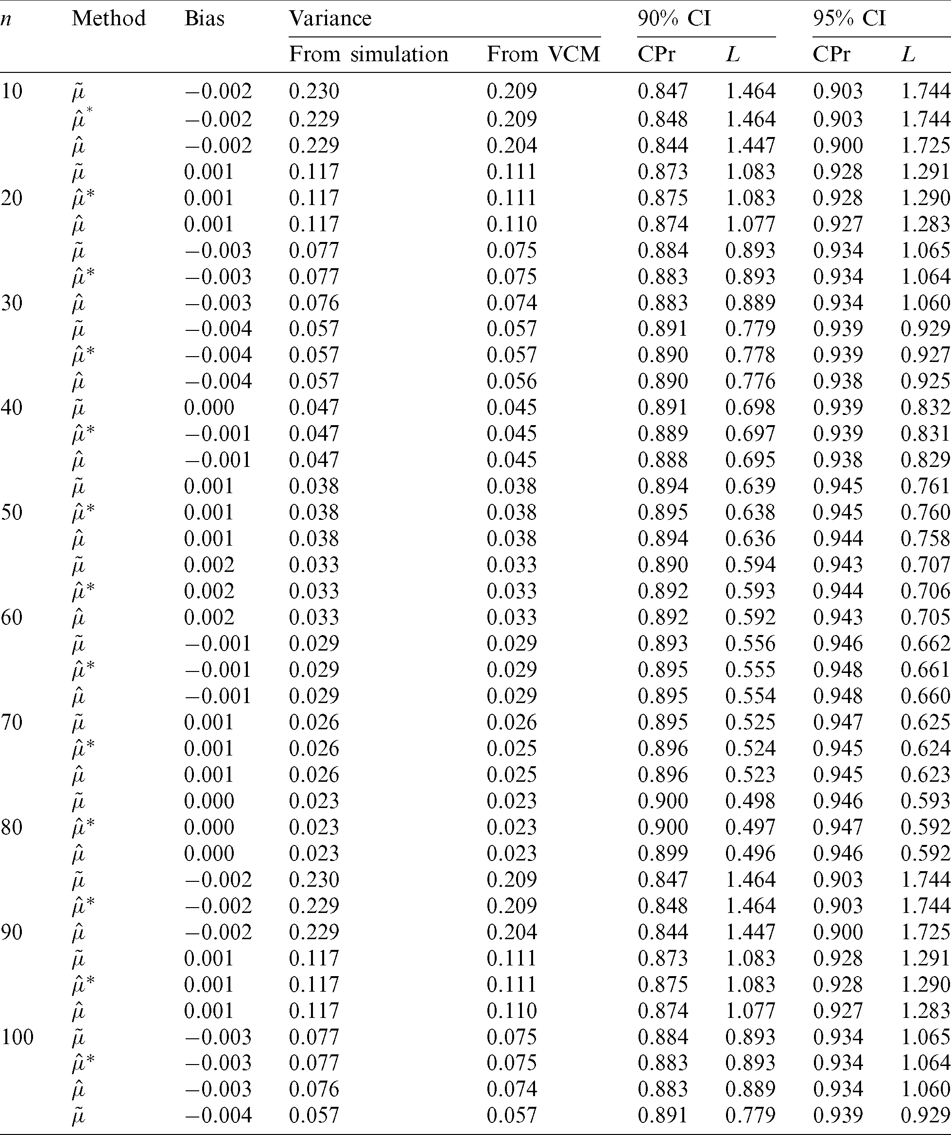
Table 2: Bias and variance for the estimators of  alongside the observed coverage probability (CPr) and length (L) of 90% and 95% confidence intervals (CIs)
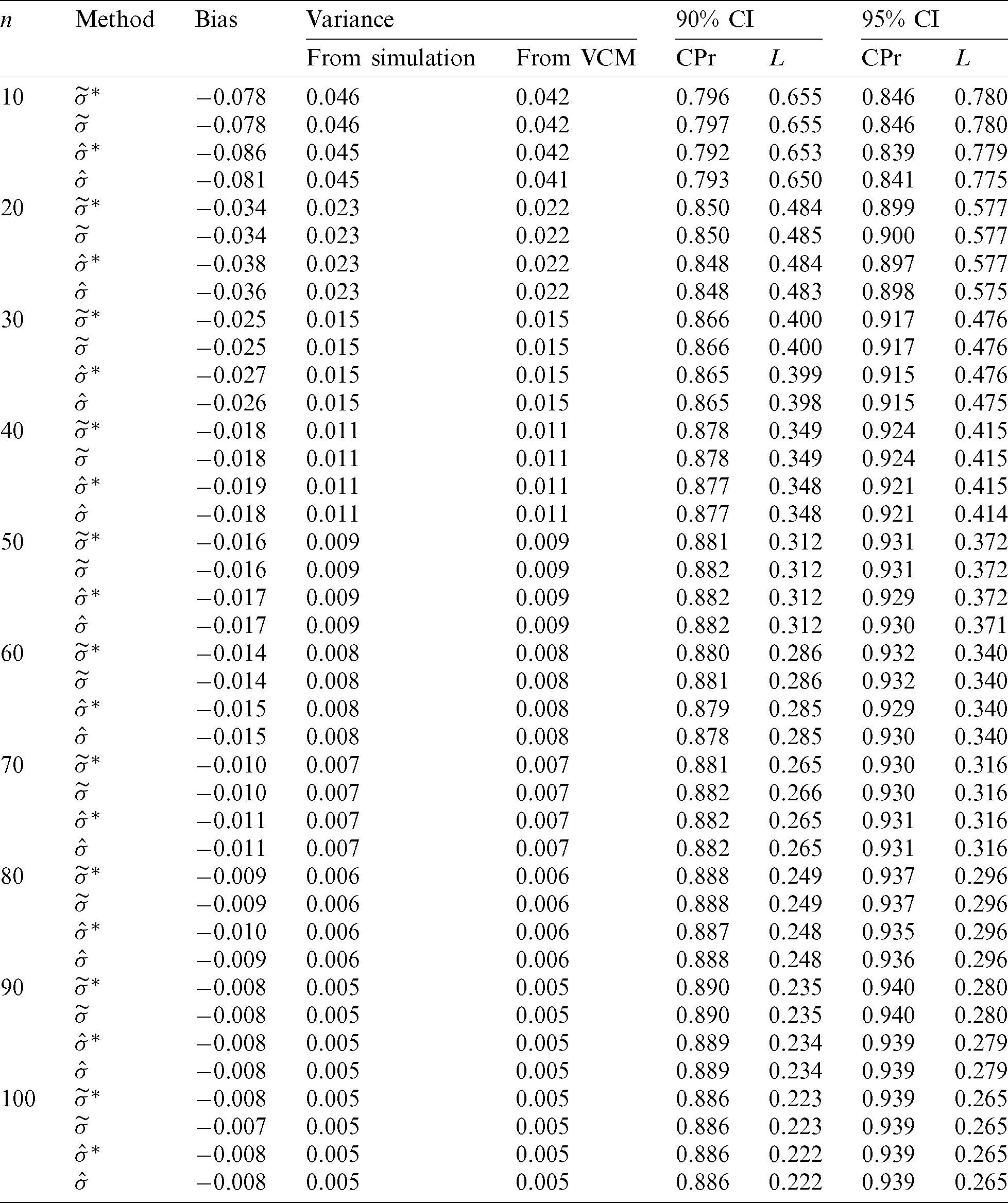
In terms of estimation efficiency, as  , both the biases and variances of the estimators tend to zero, i.e., the estimators are asymptotically consistent. Moreover, as the sample size increases, the coverage probabilities of the confidence intervals increase to the nominal levels, while the corresponding length decrease and approach zero.
In this section, two real data sets from medicine field were analyzed to illustrate the application of the AG distribution in practice. The first data under consideration represent life times (in days) of 39 patients suffering from liver cancer, and the data were reported by Elminia cancer center Ministry of Health, Egypt in (1999) [19]. The data are: 10, 14, 14, 14, 14, 14, 15, 17, 18, 20, 20, 20, 20, 20, 23, 23, 24, 26, 30, 30, 31, 40, 49, 51, 52, 60, 61, 67, 71, 74, 75, 87, 96, 105, 107, 107, 107, 116, 150.
The second data under consideration are the life times of 20 leukemia patients who were treated by a certain drug ([20,21]). The data are: 1.013, 1.034, 1.109, 1.169, 1.226, 1.509, 1.533, 1.563, 1.716, 1.929, 1.965, 2.061, 2.344, 2.546, 2.626, 2.778, 2.951, 3.413, 4.118, 5.136.
Practically, the logarithmic counterparts of these models are the normal distribution and the logistic distribution, respectively. Hence, the logarithms of the data are analyzed using the latter distributions alongside the Cauchy distribution and the AG distribution.
To determine which model appropriately fit the log-data, the minus observed log-likelihood ( ), the Akaike information criterion (
 ) [22] and the Bayesian information criterion (
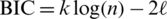 ) [23] are calculated for each model as shown in Tabs. 3 and 4. The AG distribution has provided very close results to all data sets than the normal, logistic, and Cauchy distributions. We conclude that the AG and normal distributions have outperformed the remaining ones.
Table 3: Estimators of the location  and scale
  parameters with associated SEs and the corresponding information criteria for liver cancer data
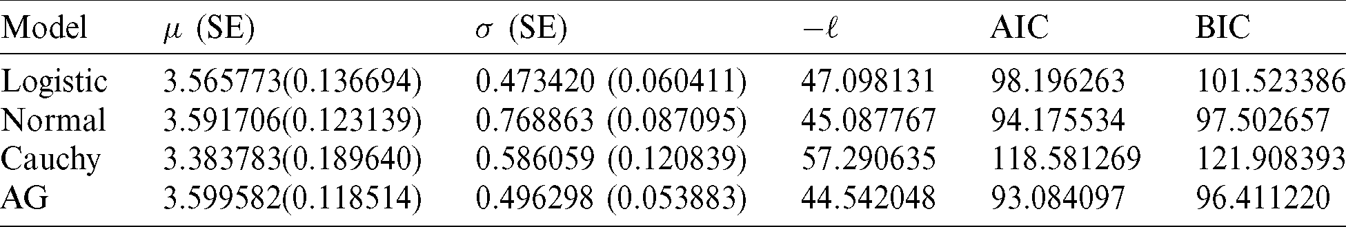
Table 4: Estimators of the location  and scale
  parameters with associated SEs and the corresponding information criteria for leukemia data
Furthermore, the empirical survival function (ESF) and the theoretical survival functions (TSF) of the AG, normal, logistic, and Cauchy distributions were compared graphically, for the two real data sets, in Fig. 4. The fitted functions of the AG model for the two real data sets including the PDF, CDF, SF and PP plots were displayed in Fig. 5.
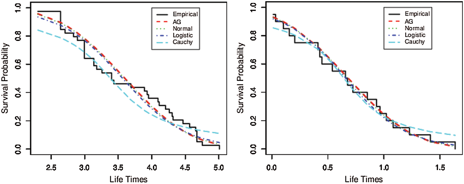
Figure 4: ESF vs. TSF of the compared distributions for liver cancer data (left) and leukemia data (right)
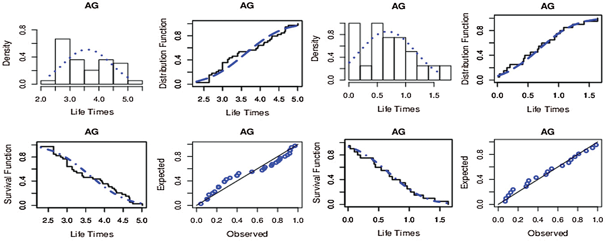
Figure 5: The fitted functions of the AG distribution for liver cancer data (left) and leukemia data (right)
In this paper, the AG distribution is considered. The relation between this distribution and the beta-normal distribution is the same as the relation between the arcsine distribution and the beta distribution. Both distribution and statistical properties of the AG distribution are intuitive and easy to verify. Point estimators for the corresponding model parameters have been obtained using the method of moments and maximum likelihood method and their asymptotic sampling distributions were discussed as well. In terms of performance, a simulation study have been conducted and its outcomes indicated that both point and interval estimators are quite similar in terms of efficiency and are asymptotically consistent as the sample size increases. In terms of data analysis, the AG distribution provided better fit to the considered data sets.
1 The superscript T denotes the matrix transpose operator.
Availability of Data and Materials: The data sets used in this paper are provided within the main body of the manuscript.
Funding Statement: The authors received no specific funding for this study.
Conflicts of Interest: The authors declare that they have no conflicts of interest to report regarding the present study.
1. C. Lee, F. Famoye and A. Y. Alzaatreh. (2013). “Methods for generating families of univariate continuous distributions in the recent decades,” Wiley Interdisciplinary Reviews: Computational Statistics, vol. 5, no. 3, pp. 219–238. [Google Scholar]
2. A. Mahdavi and D. Kundu. (2017). “A new method for generating distributions with an application to exponential distribution,” Communications in Statistics-Theory and Methods, vol. 46, no. 13, pp. 6543–6557. [Google Scholar]
3. A. Al-Babtain, M. Shakhatreh, M. Nassar and A. Afify. (2020). “A new modified Kies family: Properties, estimation under complete and type-II censored samples, and engineering applications,” Mathematics, vol. 8, pp. 1–24. [Google Scholar]
4. A. Gupta and S. Nadarajah. (2004). Handbook of beta distribution and its applications. In: A Series of Textbooks and Monographs, 1st ed., Boca Raton, London, Statistics: CRC Press. [Google Scholar]
5. P. Mörters and Y. Peres. (2010). Brownian motion. In: Cambridge Series in Statistical and Probabilistic Mathematics, 1st ed., New York, USA: Cambridge University Press. [Google Scholar]
6. N. Balakrishnan and V. Nevzorov. (2003). A Primer on Statistical Distributions, 1st ed., Hoboken, New Jersey: John Wiley & Sons. [Google Scholar]
7. N. L. Johnson, S. Kotz and N. Balakrishnan. (1995). Continuous Univariate Distributions, 2nd ed., vol. 2. New York, USA: John Wiley & Sons. [Google Scholar]
8. S. Nadarajah and S. Kotz. (2005). “On some recent modifications of Weibull distribution,” IEEE Transactions on Reliability, vol. 54, no. 4, pp. 561–562. [Google Scholar]
9. N. Eugene, C. Lee and F. Famoye. (2002). “Beta-normal distribution and its applications,” Communications in Statistics-Theory and Methods, vol. 31, no. 4, pp. 497–512. [Google Scholar]
10. S. Nadarajah. (2005). “A generalized normal distribution,” Journal of Applied statistics, vol. 32, no. 7, pp. 685–694. [Google Scholar]
11. A. Azzalini. (2005). “The skew-normal distribution and related multivariate families,” Scandinavian Journal of Statistics, vol. 32, no. 2, pp. 159–188. [Google Scholar]
12. J. Burkardt. (2014). The Truncated Normal Distribution, Florida State University: Department of Scientific Computing Website, pp. 1–35. [Google Scholar]
13. N. Balakrishnan, N. Kannan, C. Lin and H. Ng. (2003). “Point and interval estimation for gaussian distribution, based on progressively type-II censored samples,” IEEE Transactions on Reliability, vol. 52, no. 1, pp. 90–95. [Google Scholar]
14. G. S. Watson and W. T. Wells. (1961). “On the possibility of improving the mean useful life of items by eliminating those with short lives,” Technometrics, vol. 3, no. 2, pp. 281–298. [Google Scholar]
15. R. Gupta and D. Bradley. (2003). “Representing the mean residual life in terms of the failure rate,” Mathematical and Computer Modelling, vol. 37, no. 12–13, pp. 1271–1280. [Google Scholar]
16. G. Casella and R. Berger. (2002). Statistical Inference, 2nd ed., Pacific Grove, USA: Duxbury Press. [Google Scholar]
17. S. M. Ross. (2012). Simulation, Cambridge, Massachusetts, USA: Academic Press. [Google Scholar]
18. Z. Karian and E. Dudewicz. (1999). Modern Statistical Systems and GPSS Simulations, 2nd ed., Boca Raton, London: CRC Press. [Google Scholar]
19. M. M. M. Mansour. (2020). “Non-parametric statistical test for testing exponentiality with applications in medical research,” Statistical Methods in Medical Research, vol. 29, no. 2, pp. 413–420. [Google Scholar]
20. J. F. Lawless. (2003). Statistical Models and Methods for Lifetime Data, 2nd ed., vol. 362. New York, USA: John Wiley & Sons. [Google Scholar]
21. S. F. Wu and C. C. Wu. (2005). “Two stage multiple comparisons with the average for exponential location parameters under heteroscedasticity,” Journal of Statistical Planning and Inference, vol. 134, no. 2, pp. 392–408. [Google Scholar]
22. H. Akaike. (1974). “A new look at the statistical model identification,” IEEE Transactions on Automatic Control, vol. 19, no. 6, pp. 716–723. [Google Scholar]
23. G. Schwarz. (1978). “Estimating the dimension of a model,” Annals of Statistics, vol. 6, no. 2, pp. 461–464. [Google Scholar]
 | This work is licensed under a Creative Commons Attribution 4.0 International License, which permits unrestricted use, distribution, and reproduction in any medium, provided the original work is properly cited. |