DOI:10.32604/cmc.2021.014904
| Computers, Materials & Continua DOI:10.32604/cmc.2021.014904 | |
| Article |
Optimized Predictive Framework for Healthcare Through Deep Learning
1Department of Computer Science, University of Peshawar, Peshawar, 25120, Pakistan
2Department of Computer Science, Islamia College Peshawar, Peshawar, 25120, Pakistan
3Department of Computer Science, FATA University, Kohat, 26100, Pakistan
4Department of Management, College of Business Administration, King Saud University, Riyadh, Saudi Arabia
*Corresponding Author: Yasir Shahzad. Email: yasirshahzad@uop.edu.pk
Received: 26 October 2020; Accepted: 03 December 2020
Abstract: Smart healthcare integrates an advanced wave of information technology using smart devices to collect health-related medical science data. Such data usually exist in unstructured, noisy, incomplete, and heterogeneous forms. Annotating these limitations remains an open challenge in deep learning to classify health conditions. In this paper, a long short-term memory (LSTM) based health condition prediction framework is proposed to rectify imbalanced and noisy data and transform it into a useful form to predict accurate health conditions. The imbalanced and scarce data is normalized through coding to gain consistency for accurate results using synthetic minority oversampling technique. The proposed model is optimized and fine-tuned in an end to end manner to select ideal parameters using tree parzen estimator to build a probabilistic model. The patient’s medication is pigeonholed to plot the diabetic condition’s risk factor through an algorithm to classify blood glucose metrics using a modern surveillance error grid method. The proposed model can efficiently train, validate, and test noisy data by obtaining consistent results around 90% over the state of the art machine and deep learning techniques and overcoming the insufficiency in training data through transfer learning. The overall results of the proposed model are further tested with secondary datasets to verify model sustainability.
Keywords: Recurrent neural network; long short-term memory; deep learning; Bayesian optimization; surveillance error grid; hyperparameter
Advanced healthcare is an open technological facet providing multidisciplinary telemedicine treatments from basic sprains to complex chronic disease at the industry level. The vast range of eHealth innovations and applications such as interactive websites, web-portals, telehealth, e-mail, voice recognition, online health groups, and gaming are swiftly challenging the old conventional approaches [1]. The healthcare industry has tailored large scale interventions to provide affordable medical clarity through fast, reliable, robust, and recursive diagnostic techniques. Smart healthcare, therefore, falls under vertical industry areas such as very large-scale integrations, embedded systems, big data, cloud computing, and machine learning (ML) [2].
In addition to its vast scope, little attention is paid to data variance, noise, broad and scarce data in the literature. Deep learning (DL) is often rarely used with transfer learning (TL) for health related conditions. The current research proposals are consistent with ML conventional approaches, simple datasets, long delays, and open-loop problems, particularly with regard to control algorithms [3]. Subsequently, data normalization is either done manually or through conventional approaches, and nonlinear regression models are used through linear and dynamic approaches. Nevertheless, neural networks are ideal for modelling blood glucose levels using multilayer perceptrons and generative architecture DL techniques [4]. The discriminant architecture of DL embedded into TL is currently infrequent to find, especially for a diabetes prognosis. This research focuses on predicting health related issues and conditions such as diabetes and its associated diseases.
Diabetes Mellitus (DM), a dreadful disease, has affected one out of eleven adult populations globally, and up till now, it is not treated seriously. World Health Organization (WHO) depicts that the alarming figure of 463 m may rise to 578 m by 2030 and 700 m by 2045. The WHO cautions that such huge figures bring a direct financial global impact to 760b in 2019 to 823b by 2030 and 845b in 2045. Moreover, 232 m people live with this infection in undiagnosed form and have so far caused 4.2 m global deaths making it a fourth major mortality epidemic disease. Diabetes invites diverse effects on children and adults’ health, such as renal dysfunctions, cardiovascular, neuropathy, micro/macrovascular diseases, retinopathy, gums, dental, sexual, bladder, and vessels [5]. There are three different known diabetes BG states such as normal state between 80 to 130 mg/dL, hypoglycemia below 80 mg/dL, and hyperglycemia above 180 mg/dL [6]. Common symptoms of both hyperglycemia and hypoglycemia are shown in Fig. 1.
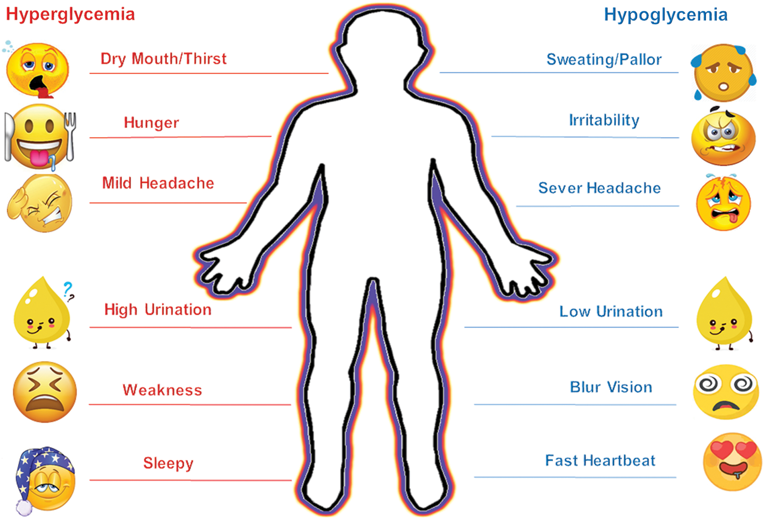
Figure 1: Common glycemic symptoms
In this research, we present a complete framework by proposing a recurrent neural network (RNN) based long short-term memory (LSTM) model to predict the patient’s past, present, and future sickness status. The proposed model has been tested for the challenging and noisy dataset (dataset-I), which is normalized to find suitable parameters for high accuracy using advanced optimization and hyperparameter (HPM) tuning. The results obtained are assessed by a surveillance error grid (SEG) to chalk out blood glucose (BG) metric. Two secondary datasets have also been trained and tested to validate the results by comparing with state of the art ML and DL techniques. We contribute to:
• Improve the accuracy rate of the predictive model and making it suitable for arbitrary nature datasets.
• Use pre-processing procedures to find fine-tuned and optimal weights for accurate results.
• Propose an easy method to train challenging data by feature engineering to increase prediction accuracy.
• Design a model that efficiently predicts illness status from the past, present, and future data relating to medication categorization, normalization, hyperparameter tuning, and accurate prediction.
The rest of the paper is organized in the following manner. Section 2 gives a recent literature review with its limitations. Section 3 has a complete methodology approach. Section 4 gives results and discussion. Finally, Section 5 concludes with future directions and limitations of this research.
Despite many efforts and achievements in the health industry, clean digital medical data remains an important and difficult challenge to obtain. Predicting accurate and productive risk factor has always been an important subject attracting many researchers’ interests. The relevant topical work is discussed below.
The authors in [7] proposed an artificial neural network (ANN) using the backpropagation and apriori algorithm to detect diabetes. An online manual system exploiting chain rule for frequent mining itemsets is proposed to detect diabetes condition. However, besides manual inputs, a simple dataset is tested to negate the involvement of doctors. No data normalization, BG metric, and TL are observed. An advanced approach is seen in [8] by proposing a DL restricted Boltzmann machine based framework to detect diabetes. The proposed work can differentiate between Type-I and Type-II diabetes by classification and recognition using decision tree ML method. Their proposed model is manual and independent between layers using a likelihood approach. However, data is input through top-down feedback with low performance and high time complexity. Three hundred data samples are selected with no clear picture of the source. Additionally, data scarcity and imbalances are not addressed. No BG metric and TL are observed.
The authors in [9] proposed a DL approach, namely GRU-D, to recover missing data for successful imputation and improved prediction. Gated recurrent unit, GRU-D is built using RNN to exploit masking and time interval in two representations of missing patterns and incorporate deep model architecture. Missing values are estimated to achieve prediction results. However, MIMIC-III dataset is selected for research with no diabetes taxonomy and cataloging, TL, and grid classification. Collaborative filtering-enhanced DL (CFDL) is proposed by [10] to build a reference system to predict future based behavior patterns. The model finds an incomplete input to predict patient readmission. However, data incompleteness and noise are addressed by ML using a traditional normalization approach. Also, no BG metric and TL are observed.
The authors in [11] proposed a model to utilize distributed and parallel computation using multiple GPU’s through DL. A large dataset of Type-2 DM is used to observe hardware and software computation complexity. However, no data optimization, categorization, TL, and error grid is seen. Decent research is observed in [12], where the authors offered RNN based LSTM with embedded TL. A Gaussian kernel is exploited using six-month continuous glucose monitoring (CGM) data of 26 participants. However, the dataset is small, and also, the error grid approach is outdated, and diabetes categorization is not observed. Another decent work is observed in [13], where authors used RNN based LSTM to estimate BG level using root mean square error (RMSE) and univariate Gaussian distribution over the output. Future forecasting is done by using the history of BG levels. However, the proposed research uses a single dataset with no trace of TL and diabetes medication categorization.
Machine learning entails high-quality training that directly depends on the quality of input data, which is not easy. The accuracy of such data can be regulated by deriving a training dataset (to predict model), test dataset (to determine the future performance of the predictive model), and validation dataset (to measure the predictive model’s adherence to a given quality standard). Healthcare is essential for the growth of many benevolence opportunities, computing fields, strength, and confidence in the health sector’s outcomes. Nevertheless, a dataset format should retain the structure and individual values in syntactic integrity so that a health practitioner may practice automated analysis.
Over twenty datasets of diabetes and their associated disease are downloaded, discussed, evaluated, and analyzed. Three datasets from the UCI ML repository are selected; a primary dataset (Dataset-1) [14] and two secondary datasets (Dataset-2, Dataset-3) [15]. The challenging and noisy dataset-I is grouped into medicinal, peculiar information, and diagnoses with a total of 101,766 instances and 50 attributes, including 47,055 male, 54,708 females, and 3 unknown genders. Simultaneously, the attributes of secondary datasets are grouped into personal information, medical tests, and keystone habits.
The primary dataset requires a detailed transformation to invoke DL abilities because insufficient information leads to inefficient models. The dataset-1 features are grouped into three categories such as patient demographic information (race, gender, age, weight, etc.), hospital metrics (number of procedures, insulin levels, number of lab procedures, H1A1c test, etc.), and diabetes medication (metformin, repaglinide, glimepiride, chlorpropamide, etc.). The extracted information and correlation between attributes are given in Fig. 2. The primary dataset contains errors, missing values, and anomalies. Preprocessing is required to gain consistency in data to prevent overfitting. The sparse properties are eliminated by auto-normalization as most fields do not have usable values, and little predictive information, as shown in Fig. 3.
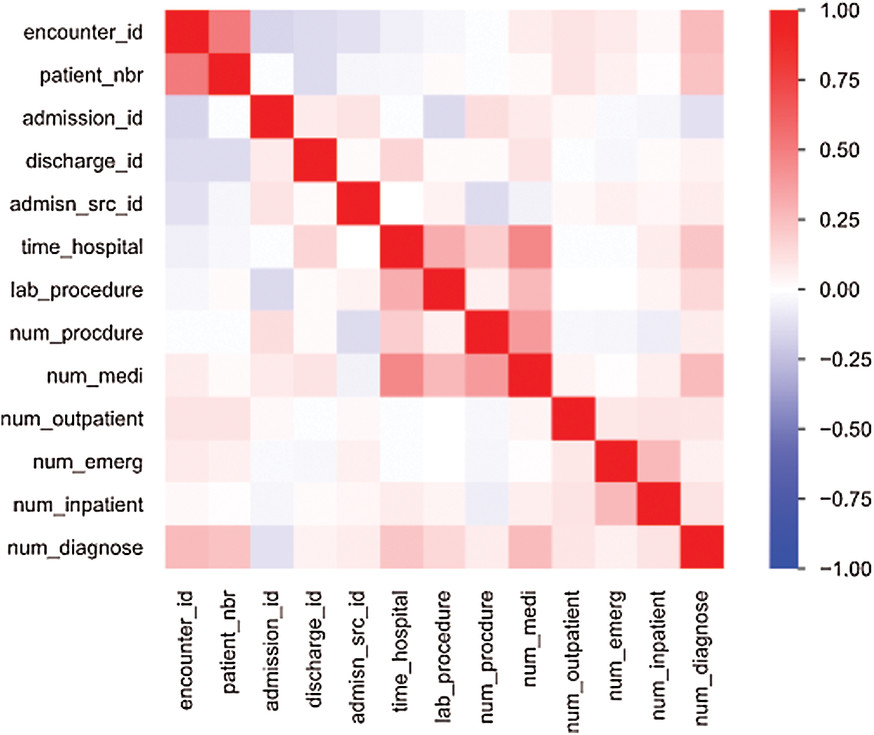
Figure 2: Pearson’s correlation coefficient (r) heatmap shows a high relationship between encounter_id and patient_nbr, time_hospital with num_medi and lab_procedure, and num_procedure with num_medi
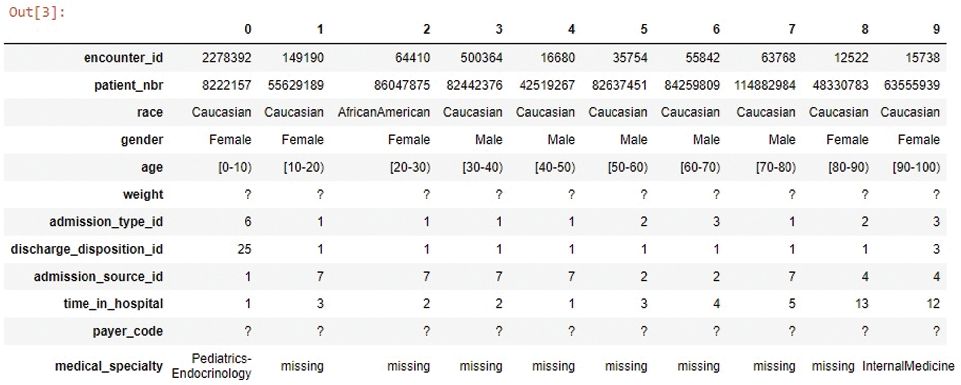
Figure 3: Weight, payer_code, and medical_specialty have high missing values
3.2 Imbalanced and Missing Values
Imbalanced data usually arise when the data is dominated by a majority class and ignoring a minority class. Hence, the dataset-I classifier routine on the minority is insufficient compared to the majority. To deal with such imbalanced data, either use the under-sampling method to balance the class and eliminate some portion of the majority class or use synthetic minority methods to increase the number of minority class instances. Synthetic minority oversampling technique (SMOTE) is preferred to create new instances rather than replicating the existing [16]. In the selected dataset, attributes having more than 50% missing values are dropped because of no significance in filling those values, as shown in Fig. 3.
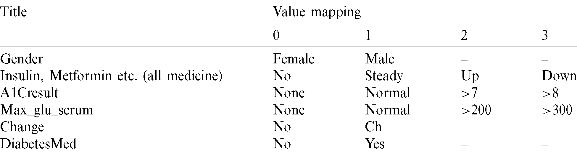
Data transformation is performed to find and map useful information  in the form of [0,1], as shown in Tab. 1. The age variable is defined by mean age interval and translated to a numeric value.
Table 1: Value mapping in dataset-I
The primary dataset includes twenty-three different medicines, which is ordered into medicinal class, as shown in Fig. 4. The categorization and classification are being carried out in consultation with medical specialists and endocrinologists for diabetic culture, current treatment trends, and diabetes medicinal groups.
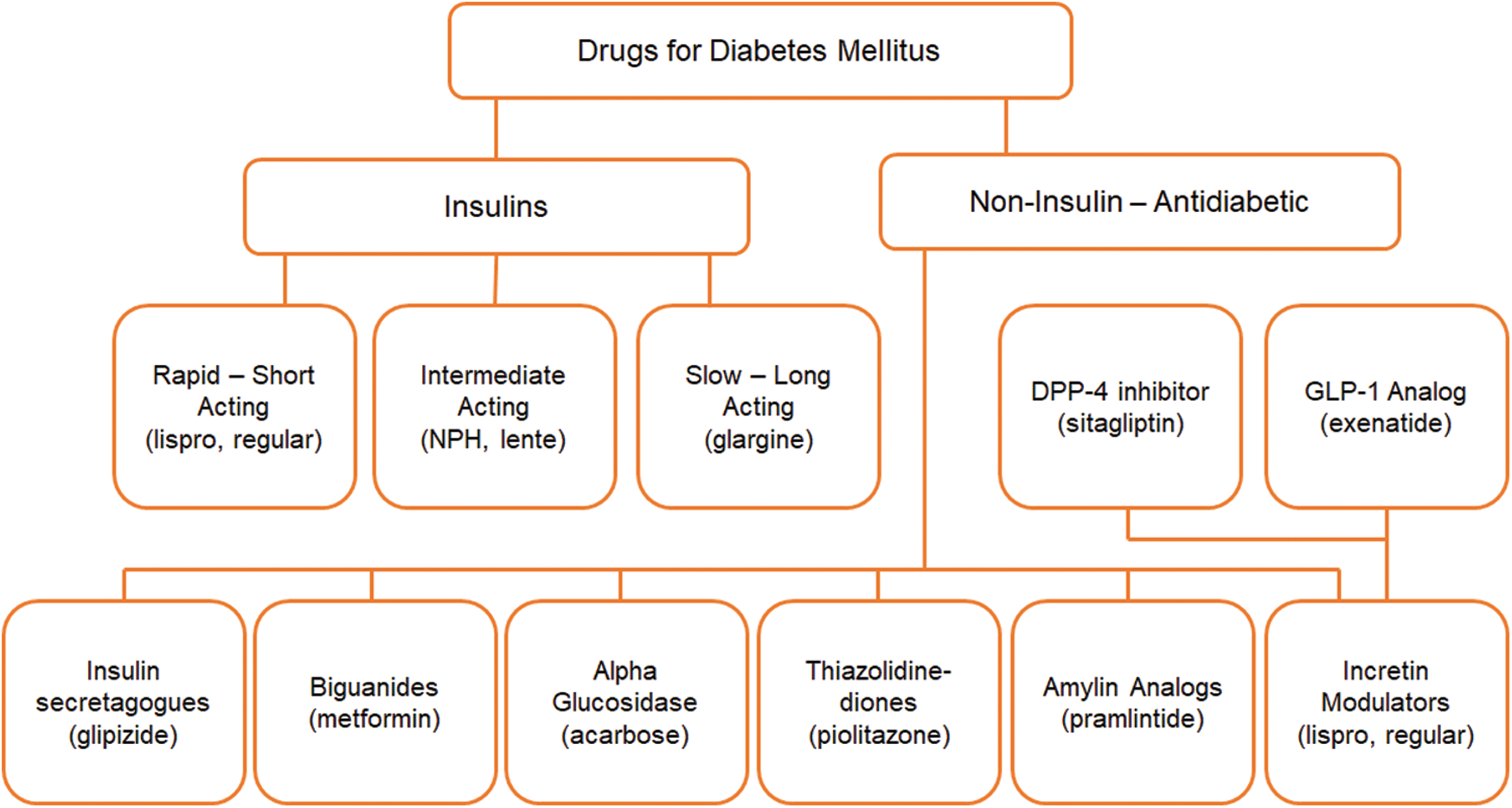
Figure 4: Diabetes medication in their standard class
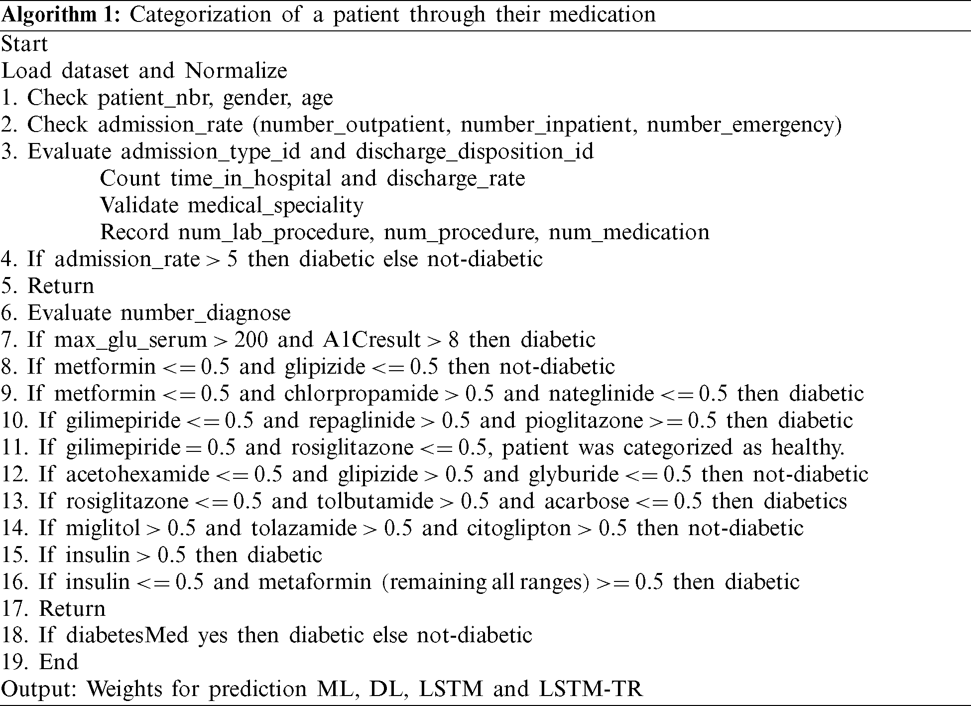
The training of a model requires a complete classification of administered medicine at home and during the hospital visit. The drug intake is added into the model, as illustrated in Algorithm 1.
The dataset value range fluctuates widely. Thus, the learning algorithm’s output can be dominated by features with higher values within a predefined limit (say Optimal Range) to retain inherent details. The Optimal Range (OR) is a set of patterns used to predict the next sequence. Min–max normalization is used to permit a configurable range to scale values in the datasets, as depicted in Eqs. (1) and (2).


where XNor is the initial value feature interest, XMin shows minimum value, XMax is a maximum value, and R denotes the optimal scaled features set [ −1,1]. To generalize the whole procedure, consider  say p1, p2, p3, p4 to predict value r of p5 with units Q1, Q2, Q3. The first module Q1 takes the input vector
  and the second module Q2 takes the input vector
  with output of first module, and so on. The final module (Q3) will predict the value rOR+3, as given in Eq. (3).

Here N is the total number of samples for time instance  and yi are the predicted and actual values. To offer perception about the working of RNN, the network typically gross an independent variable(s) X and a dependent variable y followed by the mapping and training between both X and y. The process sequence of values are
  . So, Xt has a sequence of data at time t and parameter state
  , which is equal to
  . State xt is dependent on the input parameter Xt −1, which is a previous timestamp of the model, as shown in the process model in Fig. 5.
Figure 5: Overall proposed RNN-LSTM model with TL
3.6 Model Classification and Tuning
RNN is a linear memory architecture that maintains all previous information in the internal state vector. Gradient approaches may fail when time dependencies become too long due to exponential increase or decrease in values [17]. RNN suffers from gradient vanishing, exploding, challenging training, and treating long sequencing. LSTM resolve RNN long-term dependency problem by maintaining relevant information for more extended periods and forgetting irrelevant information. LSTM also overcomes the back-flow error problems and process large datasets by keeping the cell’s information through structural gates. The proposed model uses three distinct gates; forget gate  , input gate
  , and output gate
  , as shown in Eqs. (4)–(6). The forget gate is responsible for deciding which input information from previous memory may be ignored. The input gate is responsible for feeding certain cell information. The output gate generates and updates the hidden vector
  . Additionally, LSTM allows a fourth gate called Input Modulation Gate
  , a subpart of the input gate, to reduce the learning time as a Zero-Mean for faster convergence, as shown in Eq. (7). The input gate exploits feedback weights from other memory cells in order to store or access data on its memory cell.


where  is a logistic sigmoid function to decide among [0,1] values to let it through, k is recurrent weight, m is input weight, and b is bias value. The obtained feeding back performance of LSTM is a layer at time t to the input of the same network layer at time t −1. The complete process is shown in a block diagram in Fig. 6, where information regulates using control gates kg, kf and ko by internal state ‘c.’
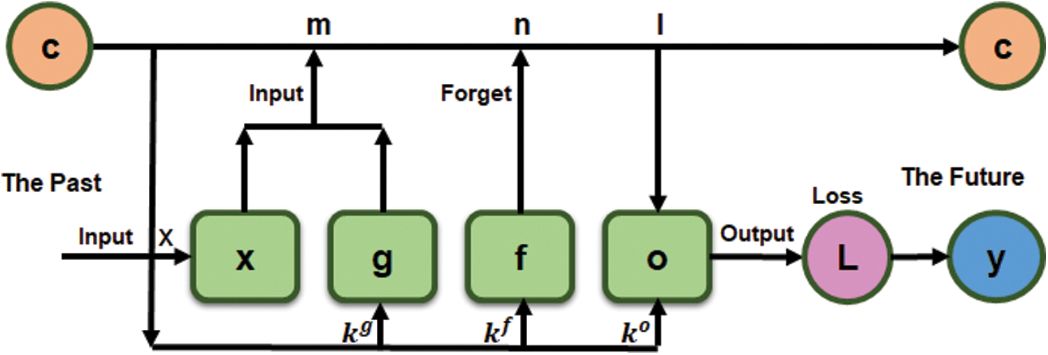
Figure 6: LSTM vector ‘x’ (The Past) a single input to predict an output ‘y’ (The Future)
3.7 Hyperparameter Optimization
Selecting ideal parameters is the key difference between average and state-of-the-art performance in a neural network because an algorithm highly depends on HPM. Various aspects, such as memory utilization and computation complexity, depend on HPM tuning, which requires more training time for significant results. HPM optimization is defined as in Eq. (8).

Here x* is the minimum generated score value,  shows that x can assume any value in the domain X and f(x) indicates the target score to reduce the validation set error. The overall goal is to evaluate model HPM producing a high score on the validation set metric. Tuning of ML algorithms is subject to trials and errors to find the optimal values, which could be either done manually or automatically. For the purpose, an automated method such as Bayesian optimization is designated to systematize finding HPM in less time using an informed search technique and assess values based on past trials. Bayesian optimization is a famous, simple, and collective approach in DL to sequentially optimize an unlabeled objective function. Bayesian’s method selection is preferred over random search optimization because the latter use long run times to assess doubtful areas of the search space [18]. Bayesian optimization allows fewer iterations to achieve excellent performance by tuning the HPM on building, training, and validating versions. Bayesian optimization is defined as in Eq. (9).

Our proposed approach use three HPM such as dropout, number of LSTM neurons, and network layer neurons. The parameter domain is defined using the hyperopt distribution function [19]. Hyperopt helps serial and parallel optimization over awkward search spaces, including real-valued, discrete, and conditional dimensions. To achieve consistent hyperopt function results, we feed input parameters to put forward to the objective function based on the Surrogate model engineering function  . The surrogate act as an approximator of the objective function to propose parameter using tree parzen estimator (TPE), Gaussian process aka GPyOpt, or random forest regression through sequential model-based algorithm configuration (SMAC). In this research, TPE is preferred over the others to build a probabilistic model of the function at each step and choose the most likewise parameters. The complete framework of the operation model, including the Bayesian optimization process, is shown in Fig. 7.
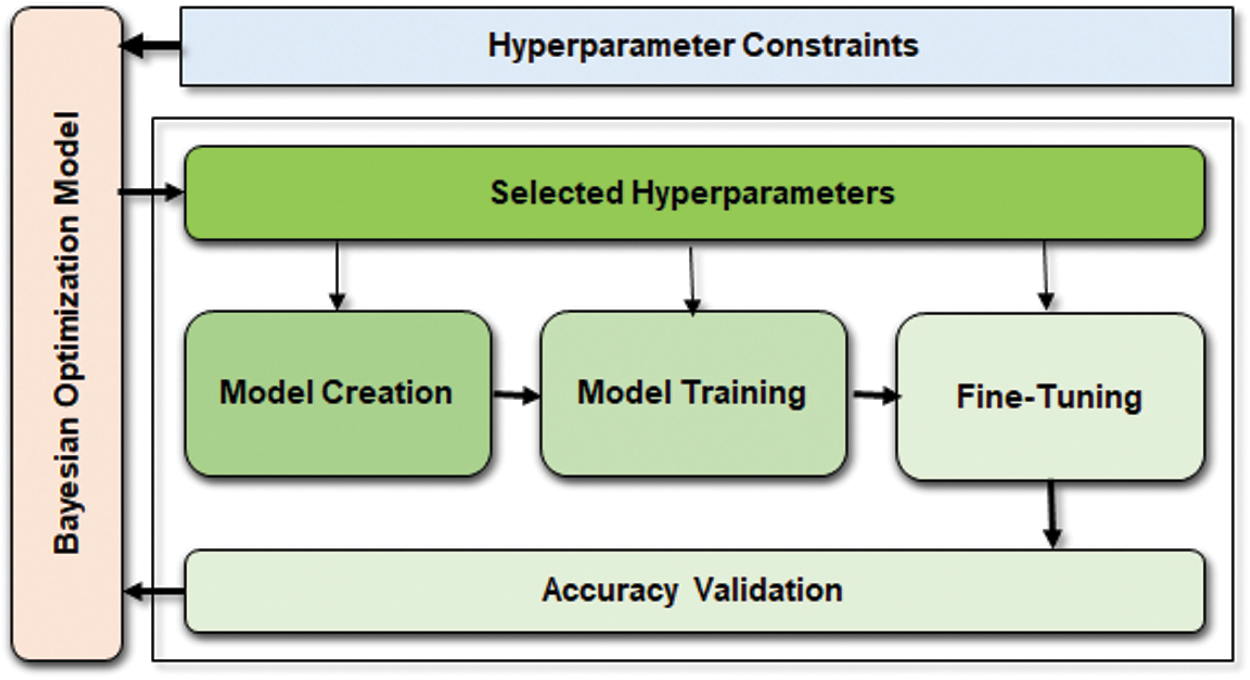
Figure 7: Bayesian optimization works on top of the predictive model to fine-tune HPM and validate accuracy. However, the weights are chosen from the HPM constraint block based on the values collected from accuracy validation
The algorithm creates a random starting point x and calculates F(x
 ). It uses trial history for conditional probability model P(
 ). Select xi giving P(
 ), resulting in better F(xi). Calculate the real value of the F(xi) and repeat steps 3 to 5 till one of the stop criteria is satisfied, for instance,
  . TPE put forward HPM by applying surrogate and selection functions. Both combine to evaluate parameters that it believes bring/calculate high accuracy on the objective function. The selection function cum TPE-Surrogate is illustrated in Eq. (10) [20]. Optimization results of LGBMRegressor, Grid Search, Random Search, and Hpyeropt optimization results are given in Tab. 2, and their comparison is given in Fig. 8.

Table 2: Comparison of search methods
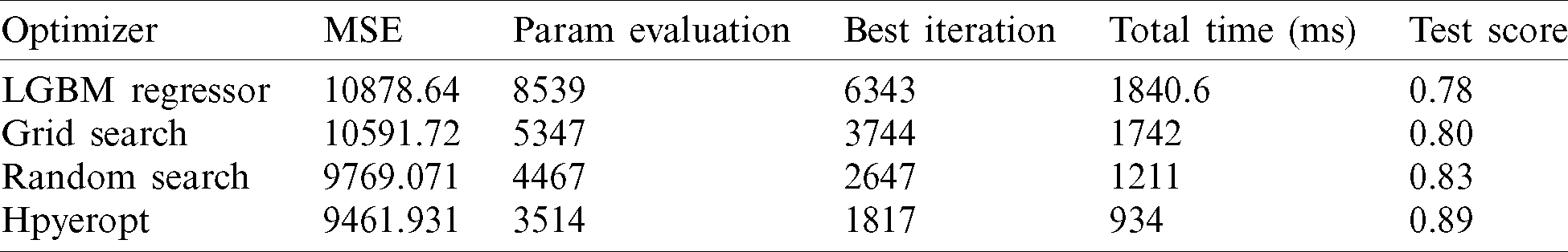
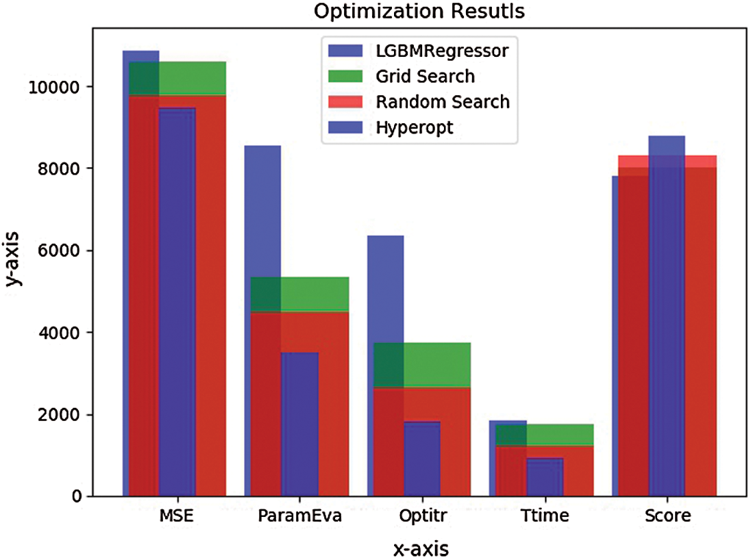
Figure 8: Optimization bar chart. The test 
LSTM can bridge time intervals and approximate noisy data to generalize over problem domains, distributed representations, and continuous values. It overcomes error back-flow problems to ensure neither exploding nor vanishing using specialized units’ internal state to reduce the input/output weight conflict. LSTM layer accompanies a dropout layer to prevent overfitting and a selected number of neurons for optimal training. In this research, the LSTM network has 512 hidden neurons and 256 neurons with an imposed dropout rate of 0.2 and 0.3 to refrain the model from over-fitting. The optimized input HPM is evaluated for 43 iterations until no improvements are seen. The output performance metrics considered are accuracy, precision, and recall to track LSTM predictive response as defined in Eqs. (11)–(13).


This research aims to build an optimized and user-friendly system that can process challenging datasets with dependent and independent variables. The optimization in autonomous mode dig deeper and draw optimal HPM for higher accuracy. More than twenty diabetes datasets are downloaded from the UCI repository having a variety of information, among which three datasets associated with each other are selected. The primary dataset is very challenging due to variation, noisy and incomplete data. To comply with data performance and accuracy, we test state of the art ML methods, as shown in Figs. 11–13. We also define two DL testing and validation methods based on straight LSTM and embedded LSTM Transfer Learning (LSTM-TL).
The RNN based LSTM is preferred because it is capable of giving more control-ability and better results. It uses extended, long multiple and parallel sequences to produce accurate results on the dataset by learning and remembering input from direct raw time series data. Additionally, 43 random seeds are trained for each HPM between 512 and 256 LSTM units; however, we went with 256 units to lower the complexity. The reason is that LSTM is a process hungry and time-consuming technique that requires error and trial approach for best suitable inputs. The proposed model is initially validated to 512 LSTM units, which consume extra operating cost and time. However, it is later on limited to 256 units for low complexity and processing. Moreover, the nature of datasets has a significant role in model performance by digging the valid inputs for dataset-I, whereas dataset-II and dataset-III are comparatively straight forward with low complexity, processing time, and operating cost.
An evaluation standard is required to define the role of the proposed model for medical practitioners. To quantify patients’ clinical accuracy, few error grid analyses are used to edge the threat of indecent future forecasts of the monitored BG levels. Previously, clarke error grid (CEG) was a standard, famous, and old technique to evaluate BG levels in clinical practices. However, it faces limitations of (i) Lack of difference between type-1 and type-2 diabetes, (ii) Discontinuous transition between Zone-B and Zone-E, and (iii) A small number of diabetes experts introduced it. A successor, namely parkes error grid (PEG), is introduced to chalk out risk zones and declare thresholds for both types of diabetes. However, PEG has no integration to the smart technology and has required a vital need to review the odd approaches w.r.t. Type-1 patient insulin pump therapy, Type-2 insulin injections, and CGM insulin injections. Henceforth, it leads us to surveillance error grid (SEG) [21]. The bilinear interpolation criterion of SEG is given as under [13].

Where  are predictive values of a patient at time t and
  are the actual values. SEG has five identified zones to discriminate emergency levels lie in each zone and eight color-defined absolute values starting from none to extreme values. Zone-1 is dedicated to emergency treatments; Zone-2 relates to oral glucose intakes; Zone-3, where no action is needed; Zone-4 shows insulin administration, and Zone-5 declares emergency treatment. The model notes that a system with
  97% inside the SEG will lie in the no-risk ‘green’ zone. It would meet the requirements of
  5% data pairs, outside the 15 mg/dL (0.83 mmol/L), over 15% standard limits. The SEG model evaluated a total of 768 samples to diagnose the BG readings (BGM) and reference values (REF) in the range of 20 to 580 mg/dl. Details are given in Tab. 3.
Table 3: Risk grade of evaluated samples in light of SEG
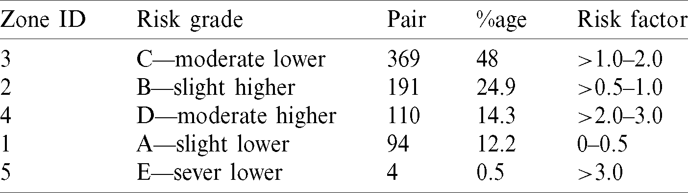
The risk factor in above mentioned table is the difference between BGM and REF as percent of  mg/dL and in mg/dL for
  mg/dL. The distribution of dataset samples that lie in various zones of the SEG plot is shown in Fig. 9.
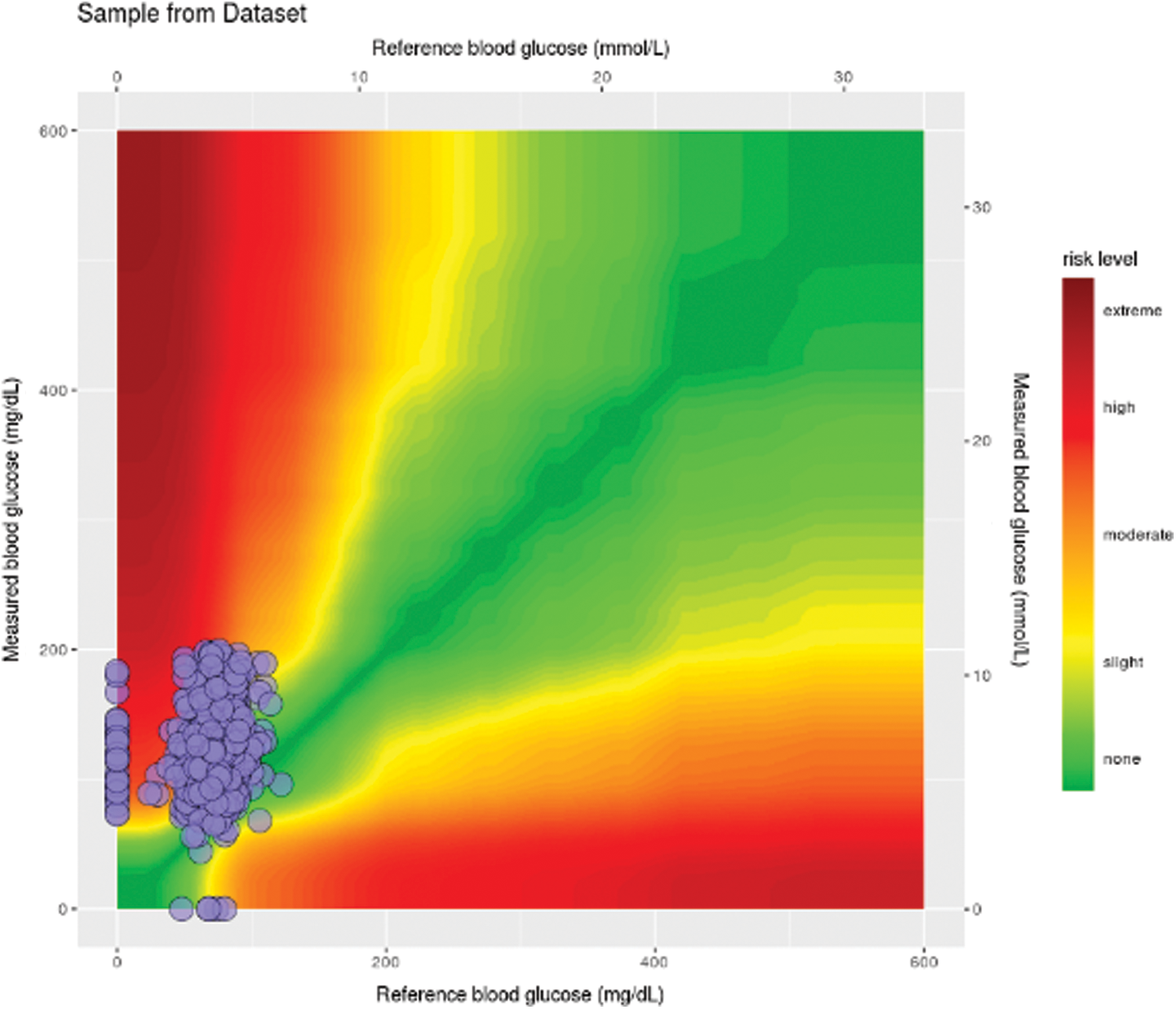
Figure 9: SEG plot showing sample risk factor
DL is a data-hungry technique to understand the hidden data patterns, resulting in high data dependency. The scale and size of a data model are in a linear relationship that shows the model’s expressive space is large enough to discover the hidden patterns under the data [22]. The proposed model performed well by a margin of significance with three input dimensions of samples, time steps, and features. An acceptable error tolerance threshold is obvious to iterate the model to reach convergence until no further improvement is seen. A 40-epochs stoppage policy is assigned to stop the validation process if no improvement is observed. Complete details of the LSTM model is given in Fig. 10.
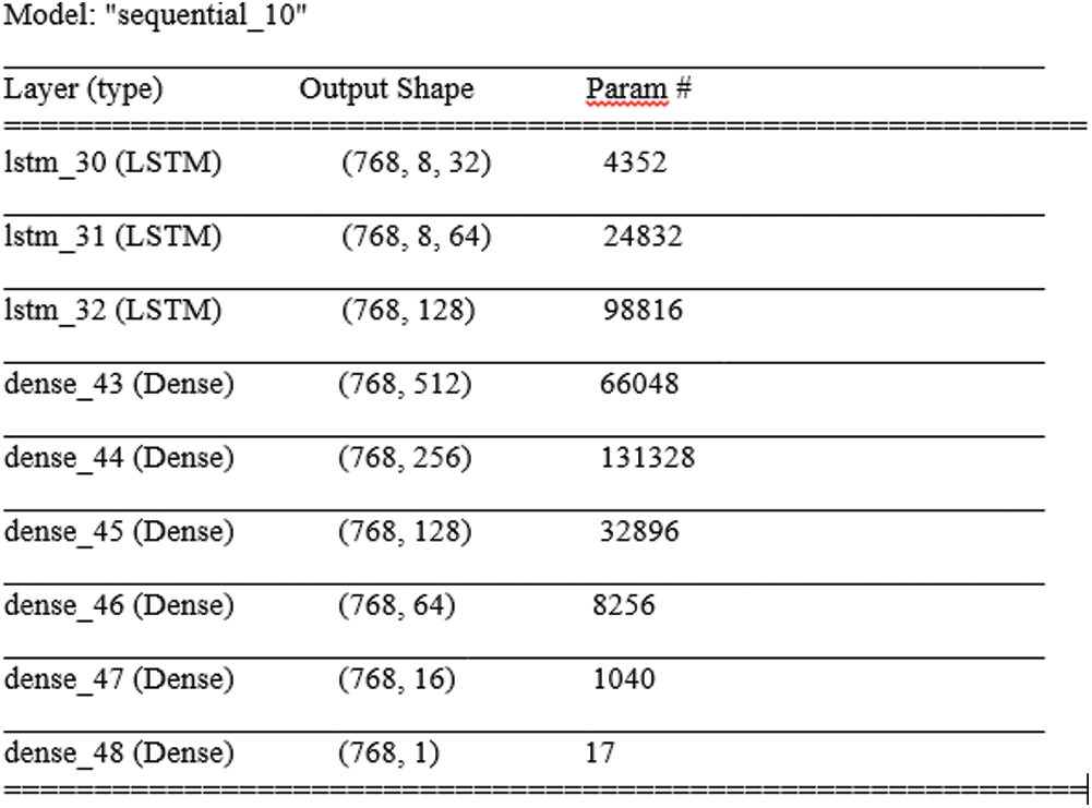
Figure 10: Param (total trainable: 367,585, non-trainable: 0)
The batch-size of LSTM output (batch-size, timespan, input) plays a vital role with a learning rate. The batch-size gradually enhanced from 128 to 768 for accurate results. The dataset distribution is set up to 60% for final training, 20% testing, and 20% validation. A maximum of 5000 epochs and 500 enforced stoppage epochs are endorsed if no improvement is observed. In order to reuse the pre-trained data on imbalanced datasets, TL is used to fit a previously unseen dataset.
The transfer learning takes up a model trained data and utilizes it on a second related task, saving time and gives better performance. TL recovers an imbalanced dataset to eliminate classification problems where several observations per class are not equally distributed. TL takes the previously trained model and freezes them. It adds additional training layers to the top of the frozen layers and trains the final model. In other words, it allows the freedom not to train the model in a target domain from scratch, which significantly lessens the demand for training data and training time [22]. However, gaps in the data lead to missing predictions. Therefore, to fill the missing values, it is not clear how much bias it would introduce. So, we propose to create the (a, b) pairs with a given history a and regression target b for a given prediction horizon. The proposed approach help to train and predict utilizing maximum data. Performance evaluation for this research is based on accuracy, area under the curve (AUC), and recall metrics, whereas precision is a supporting metric as illustrated in Figs. 11–13, respectively.
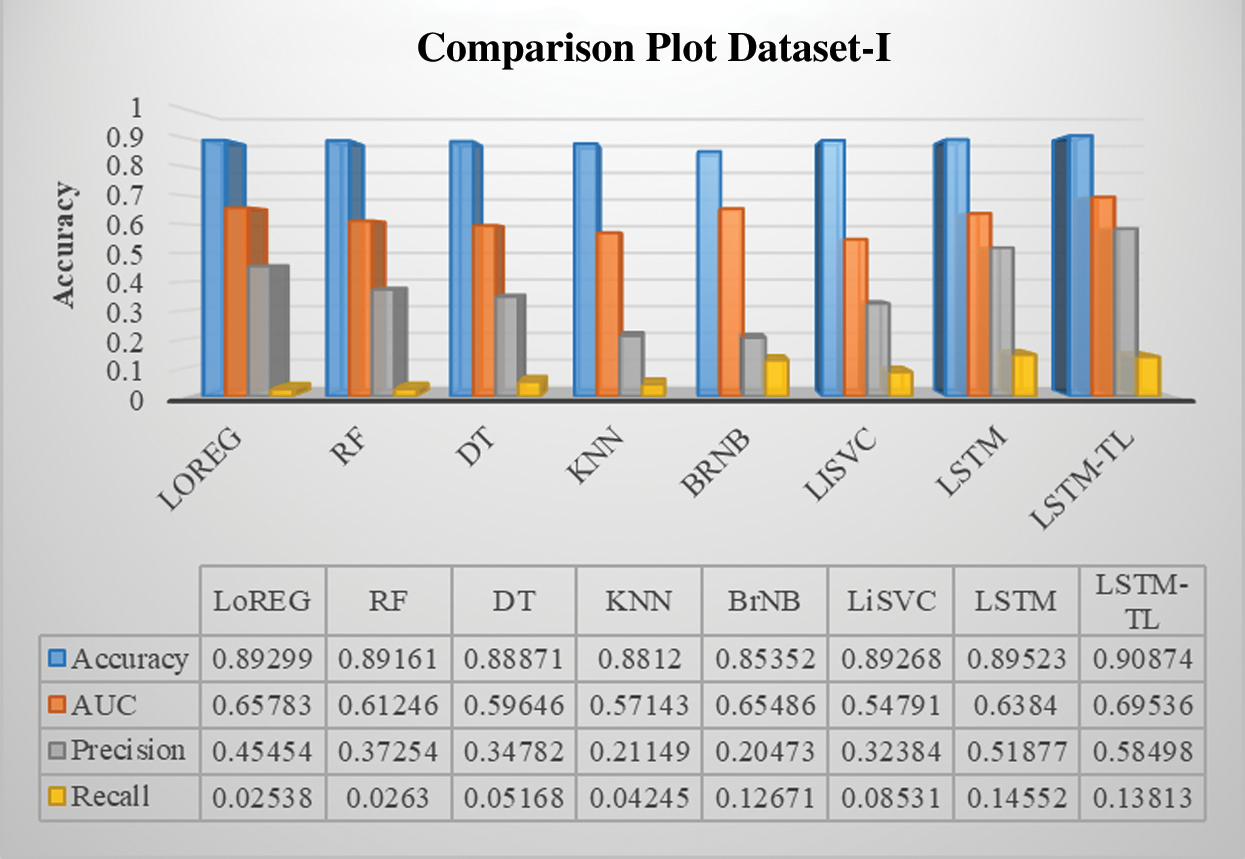
Figure 11: Performance comparison of the classifiers of DM dataset-I
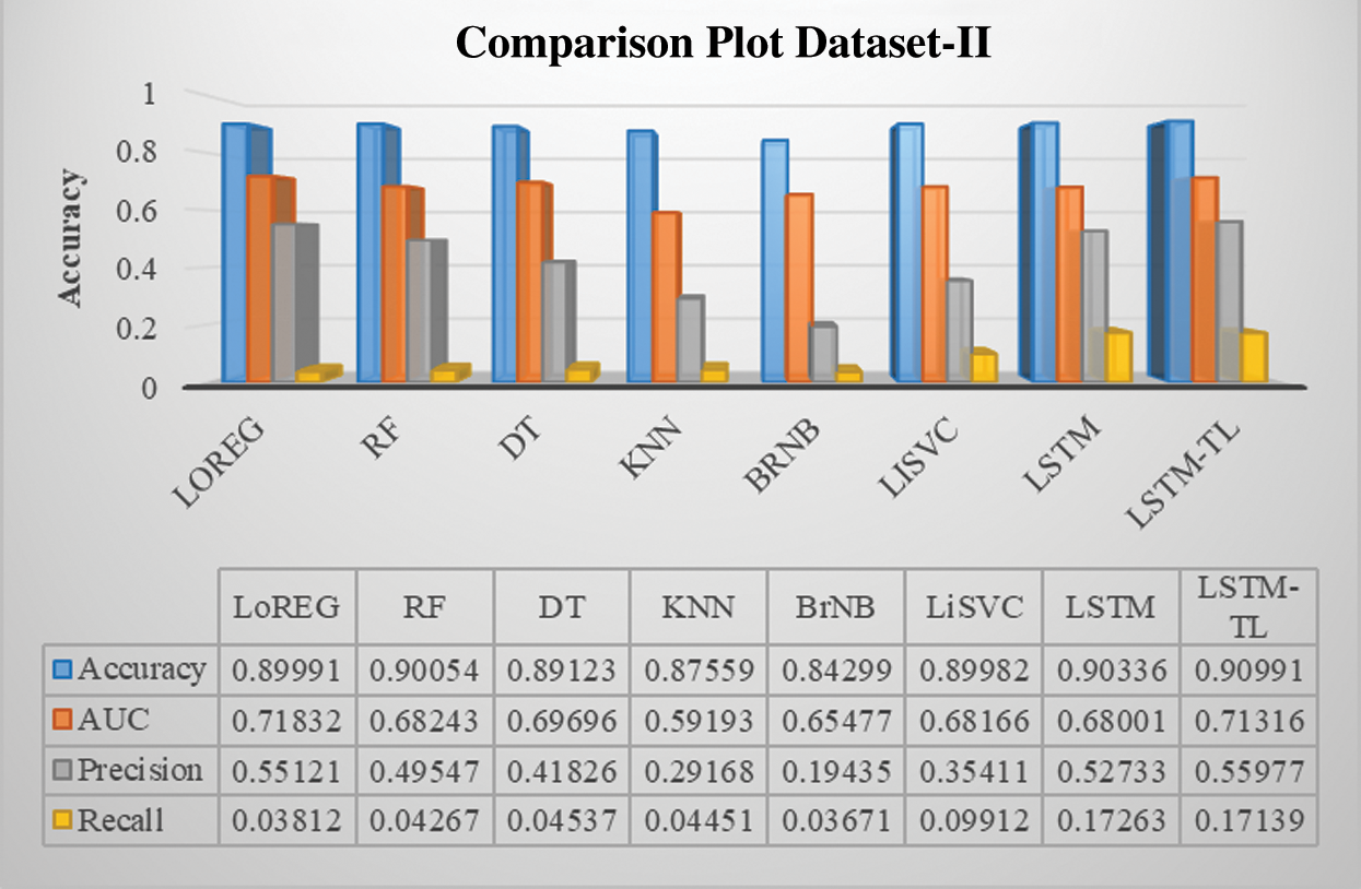
Figure 12: Performance comparison of the classifiers of renal disease dataset-II
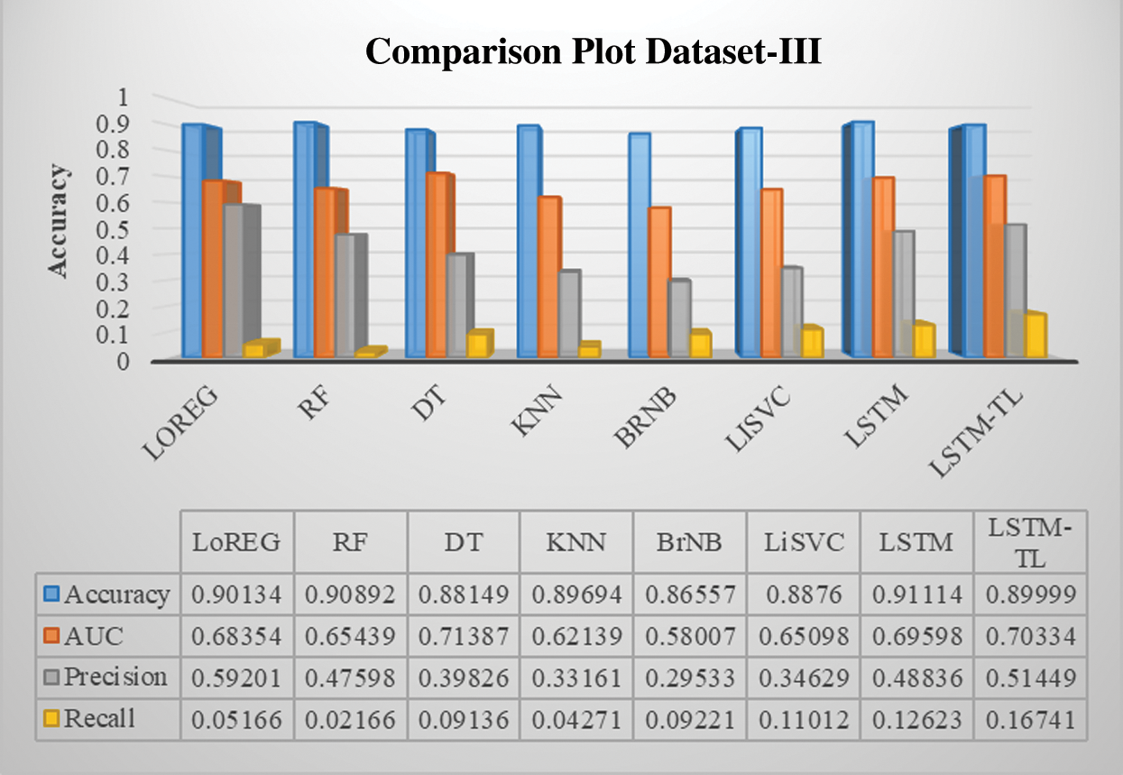
Figure 13: Performance comparison of the classifiers of cardiovascular disease dataset-III
In this study, a DL framework is proposed to assess noisy, challenging, and incomplete data through high-end optimization and diabetes patients’ evaluation. To objective our study, the data is cleaned and transformed autonomously by converting the string into numeric, categorizing fields as per their relevancy, remove data scarcity, filling empty cells, and molding medication dosage. The autonomous method is an innovative dataset experiment to improve the HPM of the proposed DL model with minimal effort. An expert level scenario is also constructed in consultation with medical specialists and endocrinologists to achieve the research objective. The dose/level of the administered medicine is classified to distinguish between normal and diabetic patients. An algorithm is designed to leverage diabetic patient data to indicate their condition and predict their future status. The objective is to develop an RNN based LSTM model to train, validate, and test data with an in-depth exploration of dynamic changes to predict BG levels. We tried to normalize the scarce dataset and equated the readings through SEG, a modern metric, for clinical risk assessments. The BG errors give the data a unique risk score compared with a reference value, which helps evaluate the risk facing by diabetic patients by successfully categorizing the samples in the specified risk zones. We hope that the obtained results will improve the clinical accuracy and further experiments, such as data points falling into custom-defined risk zones.
Previous studies concentrate on predicting BG levels, diabetic/non-diabetic status, artificial pancreas readings, glycemic control, and physiological prototypical. Keeping in view, the results of the proposed model are initially tested with state-of-the-art ML baseline models, including logistic regression, random forest, decision tree, k-nearest neighbors, naïve bayes, and linear support vector classifier. All the baseline models reveal a good and constant accuracy around 89% except for the bernoulli naïve bayes (85%), which is also an encouraging result. The overall objective is to develop a method that can guide diabetic patients to choose their healthy lifestyle according to their diabetic condition. Nutritious food and physical activity are essential elements of a healthy lifestyle. However, it is optimistic about changing lifestyles drastically, but changes come steadily.
The numerical results show that integrating TL provides better predictive accuracy, particularly when the available dataset is noisy and incomplete. It reveals significant findings in sparse data with complex trends, missing and imputed values. Before training, data is normalized and optimized to create the TL dataset to pre-train a global LSTM model. The regulated data is trained to the RNN-LSTM DL model and tested to 20% of a dataset, which is always a reasonable percentage between maintaining model accuracy and avoiding overfitting. Here, our LSTM layer(s) did all the work to transform the input to predict the desired output.
To conclude, DL systems need data to provide difficult interpretations to effectively diagnose health conditions to improve clinical decision-making uncertainty. In this paper, the RNN-LSTM model is proposed to test and forecast diabetic patients’ disease status from the demanding real-world challenging dataset with scarcity, missing/imbalanced values, incomplete, and noisy data. The data is normalized autonomously via standard procedures and value mapping. The normalized data is fine-tuned by Bayesian optimization to chalk out interstitial HPM values. The data normalization, HPM tuning, and medicinal categorizing are customized according to the proposed model, which through state of the art ML and DL methods, provide a high and consistent level of accuracy.
An algorithm specifies the primary dataset with twenty-three medicinal attributes for a dose-based patient prediction. LSTM configuration is effectively optimized for accurate input, LSTM units, and output synchronization via trial and error basis. Finally, TL is integrated into LSTM to repair imbalances and feed-forward the training data for stable prediction and higher accuracy. To validate the model’s performance, two secondary datasets are tested to ensure model consistency, reliability, and accurate performance.
The initial idea was to obtain a local dataset from the health regulatory bodies, hospitals, and laboratories for this research. However, the current COVID-19 emergency led us to use a readymade dataset for testing our proposed model. In a pilot investigation, we find that this work has significant implications for future research using a local dataset. In the future, we will collect data from local sources and prepare a pilot project by embedding sensor technology such as body area networks and generate a dataset. A complete framework will collect health data through customized software. The collected data will be normalized for accurate forecasting and bind aggregated readings with medical professionals for on-site expert advice.
1. Increasing LSTM units leads to more complexity, processing time, and operating cost
2. Old datasets. Whereas dataset-I has missing fields of Age and Weight
3. Low test precessions
Funding Statement: This work is supported by Researchers Supporting Project number (RSP-2020/87), King Saud University, Riyadh, Saudi Arabia.
Conflicts of Interest: The authors declare that they have no conflicts of interest to report regarding the present study.
1. T. Saheb and L. Izadi. (2019). “Paradigm of IoT big data analytics in the healthcare industry: A review of scientific literature and mapping of research trends,” Telematics and Informatics, vol. 41, pp. 70–85. [Google Scholar]
2. K. B. Kim and K. H. Han. (2020). “A study of the digital healthcare industry in the fourth industrial revolution,” Journal of Convergence for Information Technology, vol. 10, no. 3, pp. 7–15. [Google Scholar]
3. B. Jan, H. Farman, M. Khan, M. Imran, I. U. Islam et al. (2019). , “Deep learning in big data analytics: A comparative study,” Computers & Electrical Engineering, vol. 75, pp. 257–287. [Google Scholar]
4. N. M. Kumar and R. Manjula. (2018). “Design of multi-layer perceptron for the diagnosis of diabetes mellitus using keras in deep learning,” Smart Intelligent Computing and Applications, vol. 104, pp. 702–711. [Google Scholar]
5. I. Pearce, R. Simo, M. Lovesta-Adrain, D. T. Wong and M. Evas. (2019). “Association between diabetic eye disease and other complications of diabetes: Implications for care, A systematic review,” Diabetes, Obesity and Metabolism, vol. 21, no. 3, pp. 467–478. [Google Scholar]
6. K. Papatheodorou, M. Banch, E. Bekiari, M. Rizzo and M. Edmonds. (2018). “Complications of diabetes 2017,” Journal of Diabetes Research, vol. 2018, pp. 1–4. [Google Scholar]
7. K. Sridar and D. Shanthi. (2014). “Medical diagnosis system for the diabetes mellitus by using back propagation-apriori algorithms,” Journal of Theoretical and Applied Information Technology, vol. 68, no. 1, pp. 36–43. [Google Scholar]
8. P. T. Kamble and S. T. Patil. (2016). “Diabetes detection using deep learning approach,” International Journal for Innovative Research in Science & Technology, vol. 2, no. 12, pp. 342–349. [Google Scholar]
9. Z. Che, S. Purushotham, K. Cho, D. Sontag and Y. Liu. (2018). “Recurrent neural networks for multivariate time series with missing values,” Scientific Reports 8, vol. 6085, pp. 1–12. [Google Scholar]
10. L. Xin. (2018). “Health risk prediction using big medical data–-A collaborative filtering-enhanced deep learning approach,” M. S. dissertation, Fargo, North Dakota: North Dakota State University. [Google Scholar]
11. D. Sierra-Sosa, B. Garcia-Zapirain, C. Castillo, I. Oleagordia, R. Nuno-Solinis et al. (2019). , “Scalable healthcare assessment for diabetic patients using deep learning on multiple gpus,” IEEE Transactions on Industrial Informatics, vol. 15, no. 10, pp. 5682–5689. [Google Scholar]
12. S. H. A. Faruqui, Y. Du, R. Meka, A. Alaeddini, C. Li et al. (2019). , “Development of a deep learning model for dynamic forecasting of blood glucose level for type 2 diabetes mellitus: Secondary analysis of a randomized controlled trial,” JMIR mHealth and uHealth, vol. 7, no. 11, pp. 1–14. [Google Scholar]
13. J. Martinsson, A. Schliep, B. Eliasson and O. Mogren. (2020). “Blood glucose prediction with variance estimation using recurrent neural networks,” Journal of Healthcare Informatics Research, vol. 4, no. 1, pp. 1–18. [Google Scholar]
14. B. Strack, J. P. DeShazo, C. Genninggs, J. L. Olmo, S. Ventura et al. (2014). , “Impact of HBA1C measurement on hospital readmission rates: analysis of 70,000 clinical database patient records,” BioMed Research International, vol. 2014, no. 2, pp. 1–11. [Google Scholar]
15. D. Dua and C. Graff. (2019). “UCI Machine Learning Repository,” . [Online]. Available: https://archive.ics.uci.edu/ml/datasets/chronic_kidney_disease. [Accessed March 04, 2020]. [Google Scholar]
16. U. K. Rani, N. G. Ramadevi and D. Lavanya. (2016). “Performance of synthetic minority oversampling technique on imbalanced breast cancer data,” in 3rd Int. Conf. on Computing for Sustainable Global Development (INDIAComNew Delhi, India. [Google Scholar]
17. D. Ravi, C. Wong, F. Deligianni, M. Berthelot, J. Andreu-Perez et al. (2017). , “Deep learning for health informatics,” IEEE Journal of Biomedical and Health Informatics, vol. 21, no. 1, pp. 4–21. [Google Scholar]
18. C. W. Tsai, C. H. Hsia, S. J. Yang, S. J. Liu and Z. Y. Fang. (2020). “Optimizing hyperparameters of deep learning in predicting bus passengers based on simulated annealing,” Applied Soft Computing, vol. 88, pp. 1–9. [Google Scholar]
19. J. Bergstra, B. Komer, C. Eliasmith, D. Yamins and D. D. Cox. (2015). “Hyperopt: A Python library for model selection and hyperparameter optimization,” Computational Science & Discovery, vol. 8, no. 1, pp. 13–19. [Google Scholar]
20. P. Probst, A. L. Boulesteix and B. Bischl. (2019). “Tunability: Importance of hyperparameters of machine learning algorithms,” Journal of Machine Learning Research, vol. 20, pp. 1–32. [Google Scholar]
21. B. P. Kovatchev, C. A. Wakeman, M. D. Breton, G. J. Kost, R. F. Louie et al. (2014). , “Computing the surveillance error grid analysis: Procedures and examples,” Journal of Diabetes Science and Technology, vol. 8, no. 4, pp. 673–684. [Google Scholar]
22. J. Ahmad, B. Jan, H. Farman, W. Ahmad and A. Ullah. (2020). “Disease detection in plum using convolutional neural network under true field conditions,” Sensors, vol. 20, no. 19, pp. 1–18. [Google Scholar]
 | This work is licensed under a Creative Commons Attribution 4.0 International License, which permits unrestricted use, distribution, and reproduction in any medium, provided the original work is properly cited. |