DOI:10.32604/cmc.2021.014631
| Computers, Materials & Continua DOI:10.32604/cmc.2021.014631 | |
| Article |
Performance of Lung Cancer Prediction Methods Using Different Classification Algorithms
Department of Computer Engineering, Engineering and Architecture Faculty, Kastamonu University, Kastamonu, 37200, Turkey
*Corresponding Author: Yasemin Gültepe. Email: yasemin.gultepe@yahoo.com
Received: 04 October 2020; Accepted: 14 December 2020
Abstract: In 2018, 1.76 million people worldwide died of lung cancer. Most of these deaths are due to late diagnosis, and early-stage diagnosis significantly increases the likelihood of a successful treatment for lung cancer. Machine learning is a branch of artificial intelligence that allows computers to quickly identify patterns within complex and large datasets by learning from existing data. Machine-learning techniques have been improving rapidly and are increasingly used by medical professionals for the successful classification and diagnosis of early-stage disease. They are widely used in cancer diagnosis. In particular, machine learning has been used in the diagnosis of lung cancer due to the benefits it offers doctors and patients. In this context, we performed a study on machine-learning techniques to increase the classification accuracy of lung cancer with  sized numerical data from the Machine Learning Repository web site of the University of California, Irvine. In this study, the precision of the classification model was increased by the effective employment of pre-processing methods instead of direct use of classification algorithms. Nine datasets were derived with pre-processing methods and six machine-learning classification methods were used to achieve this improvement. The study results suggest that the accuracy of the k-nearest neighbors algorithm is superior to random forest, naïve Bayes, logistic regression, decision tree, and support vector machines. The performance of pre-processing methods was assessed on the lung cancer dataset. The most successful pre-processing methods were Z-score (83% accuracy) for normalization methods, principal component analysis (87% accuracy) for dimensionality reduction methods, and information gain (71% accuracy) for feature selection methods.
Keywords: Lung cancer; machine learning; dimensionality reduction; normalization; feature selection
An estimated 9.6 million people worldwide died of various types of cancer in 2018 and lung cancer was the leading cause of death among cancer patients (Tab. 1) [1]. Lung cancer often progresses silently. The disease cannot be detected even in late stages which significantly reduces the chances of successful treatments for patients. Therefore, it is vital to know the symptoms of lung cancer as an early-stage diagnosis significantly increases the survival rate for patients. Computational methods and techniques such as machine learning are often used in medical applications to overcome some of these challenges and to provide dependable information for diagnoses. Machine learning is the generic name for computer algorithms that model a problem according to the data of that problem. It can improve the estimation of results with classification techniques that are based on the organized data in predetermined categories [2,3]. Machine-learning classification algorithms are focused on the most economical use of the maximum possible amount of data to achieve the highest success and performance [4]. The architecture of machine-learning methods and the statistical distributions of the observed data typically lead to the training of classification models realized by minimizing a loss of function [5]. The classification algorithm is subsequently trained on the dataset to find the connection between input variables and the output. The training is considered complete when the algorithm reaches an adequate level of accuracy and the algorithm is next applied to a new dataset.
Table 1: Cases and deaths for different cancer types in 2018 [1]

The combinatorial use of different machine-learning algorithms in medical applications provides effectiveness and efficacy by making use of the specific advantages of each algorithmic technique while avoiding their disadvantages [6]. Aliferis et al. [7], for example, reported that gene expression data combined with machine-learning algorithms can lead to excellent diagnostic models of different types of lung cancer even with very modest sample sizes and very low sample-to-feature ratios. Similarly, linear regression, decision trees, gradient increasing machines, support vector machines, and community learning techniques have been successfully applied to estimate the survival time of patients to classify lung cancer patients [8]. A diagram that summarizes the overall approach of machine learning for this study is shown in Fig. 1.
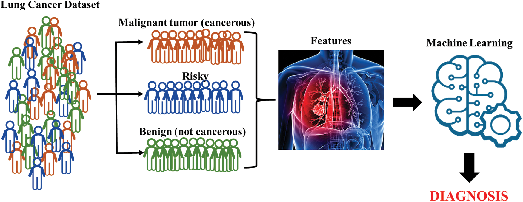
Figure 1: General diagram of machine learning
The purpose of the data pre-processing is to simplify the training and testing process by appropriately transforming the entire dataset. This is done by bringing outliers and scaling properties into an equivalent range. Pre-processing is an important stage before training machine-learning models since pre-processing applications allow machine learning to deliver better results [9]. The most used pre-processing applications are normalization, dimensional reduction of data, and feature selection. Normalization and dimensional reduction of data provide efficient, quick, and effective classifications through input and output of the prediction model in a single order in machine learning [4].
The Minimum–Maximum (min–max) normalization technique executes a linear transformation on the data. The minimum is the smallest value that data can accept and the maximum is the largest value that the data can receive. The data are usually in the range of 0–1 [10]. The Z-score normalization method uses the average and standard deviation values of the data under consideration. It is typically utilized to perform the operations with the data at normal intervals with normalized values and to obtain more meaningful and easily interpreted results [11].
Principal component analysis (PCA) is a transformation technique that reduces the size of the p-dimensional dataset that contains associated variables to a lower-dimensional space that contains uncorrelated variables. It maintains the variability of the dataset as much as possible. The variables obtained by transformation are called basic components of the original variables. The first principal component captures the maximum variance in the dataset, and the other components capture the remaining variance in descending order [12,13]. The goal of the linear discriminant analysis (LDA) is to avoid over-alignment and also to project a dataset into a lower-dimensional space with good class separability to reduce computational costs. In addition, LDA is used to maximize the distance between classes. There is no class concept in PCA because it only reduces the feature size by maximizing the distance between data points. Likewise, LDA reduces the size of the dataset by maximizing the difference between classes. LDA is used for classification problems while PCA is used for clustering problems. LDA approximates the distance of the projections on the geometric plane of the observations in the same classes in an educational sample. It can be used to create more classifying models by normalizing the data in the training sample [14,15].
Feature selection is applied to reduce the number of features in many applications where the data have hundreds or thousands of properties. The main idea is to find globally the least reduction or, in other words, the smallest set of features that represent the most important characteristics of the original set of features [16].
The choice of methods for the machine-learning prediction system is important because there are many machine-learning algorithms used in practice for particular purposes. For instance, random forest (RF) works with the logic of increasing the accuracy of results by deriving multiple decision trees while k-nearest neighbors (k-NN) uses similarities to find neighbors when classifying by majority vote. Naïve Bayes (NB) maintains the most appropriate classification by preserving the dependence of the qualifications on a particular class. Logistic regression (LR) finds the dependent and independent relationships between the variables affected by the dependent variables. Decision tree (DT) is the preferred learning method with a created tree structure since it is faster, easier to interpret, and is more effective. Support vector machines (SVMs) work with hyperplanes to separate data classification into a multidimensional space [4,17]. k-NN has been reported to give the best results for machine-learning algorithms applied to the histopathological classification of non-small cell carcinomas. The DT algorithm was reported to give the least favorable results [18].
This study aims to develop predictive models to diagnose lung cancer disease based on a customized machine-learning framework. This approach involves examining the different degrees of success of these models and analyzes their generally valid classification performances according to measurement metrics. In this context, this study consists of three modules. The first module is based on the application of the data pre-processing techniques (dimensionality reduction methods, normalization techniques, and feature selection methods) to the lung cancer dataset (LCDS), which is taken from the Machine Learning Repository website of the University of California, Irvine (UCI). The second module focuses on the demonstration and discussion of the performance of the machine-learning algorithms (RF, k-NN, NB, LR, DT, and SVMs). The third module looks at the results of all the performance measurement metrics and performs validation analysis. The aforementioned methods are widely used in diagnosis and analysis to make decisions in different areas of medicine and research.
Machine learning has many advantages. However, the process results can be affected by factors such as the dataset, the features, the determination of the learning algorithm, and the parameters of the algorithm. The lung cancer dataset used in this study was taken from the Machine Learning Repository web site of the University of California, Irvine [19]. The LCDS includes records of 56 features of 32 samples (patients) and is thus composed of 32 * 56 sized numerical data. The dataset comprises many features including age, gender, alcohol use, genetic risk, chronic lung disease, balanced diet, obesity, smoking, passive smoking, chest pain, blood cough, weight loss, shortness of breath, difficulty swallowing, snoring, and others. The massive data have been restructured by assigning the column averages of the sample to the N/A (null) value(s) in the dataset. The first column contains a classification label (category) for each sample. Three values are given for the classification in lung cancer data: 1 for malignant tumor (cancerous), 2 for risky, and 3 for benign (not cancerous).
The dataset was randomly split into 80% for training and 20% for the test in this study to give the best results from the machine-learning applications. The tested data were used to determine the success of the system, namely, how close the values from the model obtained with the training data are to the actual values.
2.2 Normalization and Dimensional Reduction of Data
One of the fundamental problems encountered in machine learning applications is the regulation of the data. All numerical values in the dataset may not be in same range and for this reason an imbalance between the values can dominate the target values. Normalization methods are applied to eliminate possible problems of this type. The most commonly used min–max and Z-score normalization techniques were used to observe the effect of normalization techniques on prediction of machine-learning methods in diagnosis of lung cancer disease and to determine the most appropriate normalization technique in the study.
A high number of attributes increases the data dimensionality but brings with it problems of analysis and classification. Therefore, this type of approach requires a dimensionality reduction. The most preferred methods for dimensionality reduction are PCA and LDA [20]. PCA and LDA reduction methods were used in the present study.
The features in the datasets are one of the most important factors affecting the performance of the classification. Sometimes, the low number of features causes the classes to not separate properly. In the case of many features, there are problems such as an increase in training time and a decrease in the accuracy rate of the many noise-related features [16]. Feature selection is aimed at finding individually the best features that maximize the ability for classification from a large group of features [21]. Feature selection is critical for machine-learning in cancer diagnosis. Therefore, four feature selection methods were used within the scope of the application to determine the prediction properties: Chi-square, information gain, forward selection, and relief.
Chi-square ( ) is based on statistics and is widely used in feature selection processes. The
  test is based on whether the difference between observed frequencies (O) and expected frequencies (E) is statistically significant. The
  test uses data specified as qualitative or ordinal variables. Furthermore,
  can be applied by qualifying continuous variables specified by measurement as more or less than a certain degree. The test is not possible if the data are expressed as percentages or percentages [22]. The
  formula is as follows:

Abbreviations:  ,
,  ,
,  observed frequency for
  th attribute,
  expected frequency affirmed by the null hypothesis for the
  th attribute.
Information gain (IG) is one of the most popular feature selection techniques. The principle of selecting a feature is based on finding the most set of features for the classes. It is an entropy-based feature selection algorithm and the IG coefficient is calculated for each attribute. The feature sets with the highest IG coefficient are selected [23]. This method is represented as follows:

Abbreviations:  ,
,  ,
,  ,
,  .
.
The purpose of the forward selection (F) is to find features that maximize the objective function. There is an objective function J, for which as attempt is made to maximize its value, and this function depends on a subset of the F properties. The algorithm starts by initializing F
 to an empty set, and the method requires several features to select (k) and the original feature set (F). Let Xj be a random parameter for feature j and Y be the parameter that decides the class label (e.g., cancerous vs. not cancerous). The first step is to find the feature Xj that maximizes the aim function J that takes in arguments Xj, Y, and F
 . Feature Xj that maximizes the aim objective function is added to F
 and removed from F. This process is repeated until the cardinality of F
 is k [24].
Relief (W) finds the value of properties by trying to reveal the dependencies between properties in binary classification problems [25]. Each feature in the dataset is scaled to the range [0 1]. The algorithm is repeated m times and each time the weight vector is updated as in Eq. (3):

Abbreviations:  ,
,  ,
,  closest instance of the same class,
  closest instance of the different class.
2.4 Machine Learning Classification
In the classification process, RF, k-NN, NB, LR, DT, and SVM algorithms were applied to the dataset. Python 3.6 programming language was used for software “Anaconda,” a data science platform that supports the Python language, was used in the study. The ‘numpy’ and ‘pandas’ libraries were preferred during the build-up of all modules for practicing on the enormous data. The model parameters of the six machine-learning algorithms and their values were assigned as in Tab. 2.
Table 2: Model parameter values
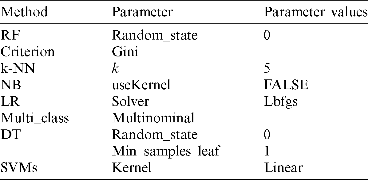
Abbreviations: RF, Random forest; k-NN, k-nearest neighbors; NB, Naïve Bayes; LR, Logistic regression; DT, Decision tree; SVMs, Support vector machines.
The flow diagram for the research study is shown in Fig. 2. The raw data were pre-processed and an attempt was made to use the first module to determine the prominent features and criteria for lung cancer. These applied pre-processing techniques were used to make an appropriate analysis and see if they were suitable for classification of collected data. They gave better accuracy for classification. In the second module, the datasets created by going through the different pre-processes were classified with machine-learning algorithms. The results obtained were analyzed and evaluated for accuracy in the third module.
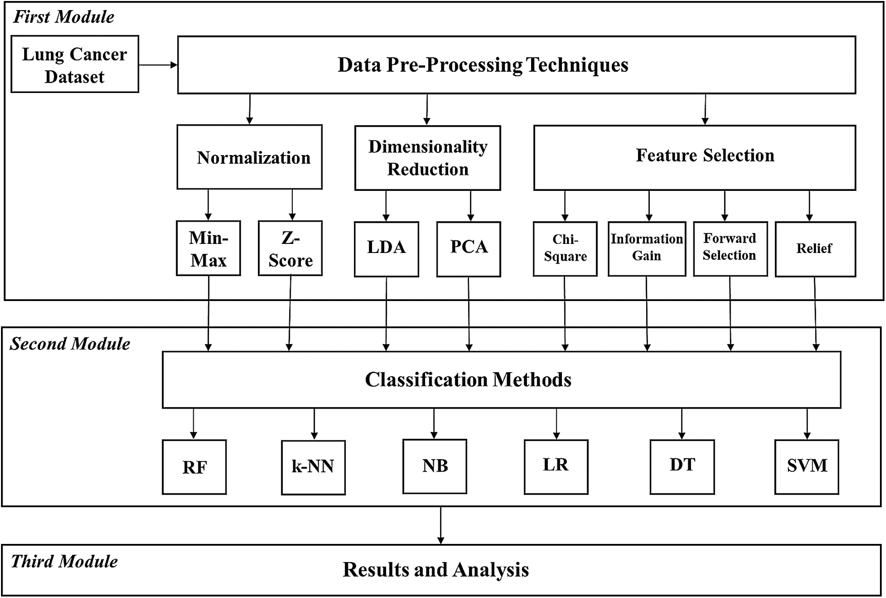
Figure 2: Flow chart of the proposed approach (Abbreviations: Min–Max, Minimum–Maximum; LDA, Linear discriminant analysis; PCA, Principal component analysis; RF, Random forest; k-NN, k-nearest neighbors; NB, Naïve Bayes; LR, Logistic regression; DT, Decision tree; SVM, Support vector machine)
The logic behind RF is to increase the accuracy of the results by deriving multiple decision trees. k-NN uses similarities to find neighbors when classifying by majority vote. NB maintains the most appropriate classification by preserving the dependence of the qualifications on a particular class. LR finds the dependent and independent relationship between the variables affected by the dependent variables. DT is the preferred learning method with a created tree structure owing to its faster, easier to interpret, and more effective results. SVM works with hyperplanes to separate data classification in multidimensional space [4,17].
The model performance criteria used are root mean square error (RMSE) and mean absolute error (MAE). The formulations of these are given in Eqs. (4) and (5), respectively:


RMSE is an indicator used to determine the error rate between the measured values and the values estimated by a model. Therefore, the closer RMSE approaches to zero the more it indicates that the predictive power of the model has increased. MAE is used to indicate the absolute error between the measured values and the values predicted by the model. Like RMSE, the closer MAE approaches to zero the more it indicates that the predictive power of the model has increased [13,26].
There are two important steps for the prediction: one is to prepare the data to estimate; the other is to compare the predictive models. The criteria for the comparison of the models include accuracy, speed, robustness, scalability, interpretability, and performance.
The accuracy values of RF, k-NN, NB, LR, DT, and SVM algorithms were calculated as 0.14, 0.71, 0.71, 0.57, 0.71, and 0.43, respectively. These values were obtained in calculations made with the raw data. The best results were obtained with k-NN, NB, and DT algorithms, while the worst results were found with the RF algorithm. Similarly, other researchers have achieved successful results with machine-learning algorithms in a wide range of studies including, for example, the following: cancer prognosis and prediction [27], leukemia, colon, and lymphoma [28], breast cancer diagnosis and prognosis [29–31], prediction of future gastric cancer [32], gene selection for cancer classification [33], skin cancer detection [34], cervical cancer diagnosis [35], pancreatic cancer [36], prostate cancer [37,38], precision medicine for cancer [39], and classification of lung cancer stages [40]. The research results show that k-NN, NB, and DT algorithms can predict lung cancer with increased precision and success.
The raw data were compared for min–max and Z-scores (Tab. 3). Min–max and Z-scores returned better results in LR, SVM, and k-NN calculations compared to the raw data. However, the performance in NB and DT calculations for min–max and Z-scores was decreased.
Table 3: Accuracy, RMSE, and MAE values of machine-learning classifiers using Min–Max and Z-score

Abbreviations: RF, Random forest; k-NN, k-nearest neighbors; NB, Naïve Bayes; LR, Logistic regression; DT, Decision tree; SVMs, Support vector machines; RMSE, Root mean square error; MAE, Mean absolute error.
The best results were an accuracy of 0.83 and an MAE value of 0.17 for k-NN, which calculates using the properties of the Z-score. The worst results were an accuracy of 0.29 and an MAE value of 0.71 for NB, which calculates using min–max properties. The accuracy level of normalization techniques and the raw dataset is given in Fig. 3. Jain et al. [41] reported that Z-score gives positive results on the data complexity measures. Nonetheless, Z-score performed successfully for leukemia [28]. In addition, Z-score has increased performance at 0.12 compared with the raw dataset for the k-NN algorithm used in the study.
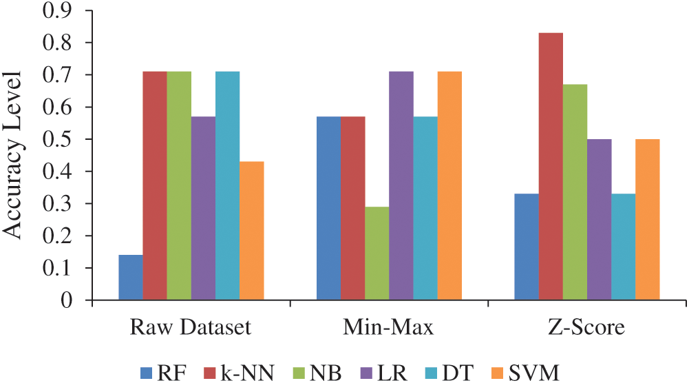
Figure 3: Accuracy level of normalization techniques and raw dataset (Abbreviations: Min–Max, Minimum–Maximum; RF, Random forest; k-NN, k-nearest neighbors; NB, Naïve Bayes; LR, Logistic regression; DT, Decision tree; SVM, Support vector machine)
Fifty-six features in LCDS were reduced to 30 features using PCA and LDA, which thus saved processing time. Overall, there was an increase in the accuracy of the calculations made by PCA, and the best result of 0.87 was found for NB, and the worst result of 0.57 was found for DT. The accuracy levels of all the calculations made with LDA decreased according to the calculations made with the raw data (Tab. 4).
Table 4: Accuracy, RMSE, and MAE values of machine-learning classifiers using PCA and LDA

Abbreviations: RF, Random forest; k-NN, k-nearest neighbors; NB, Naïve Bayes; LR, Logistic regression; DT, Decision tree; SVMs, Support vector machines; RMSE, Root mean square error; MAE, Mean absolute error; LDA, Linear discriminant analysis; PCA, Principal component analysis.
The accuracy level for the dimensional reduction methods and the raw dataset are given in Fig. 4. PCA provided a high degree of accuracy in tumor, glioma, lung, colon, and breast cancer datasets [42]. The classification performance was increased in the lung cancer study using PCA although the number of attributes decreased more than one and a half times. In this way, the computational cost and complexity of the classification process were greatly reduced with PCA [43]. Bhaskar et al. [21] reported that PCA gives superior results with NB than k-NN. Similarly, the best accuracy level was found for the NB algorithm with PCA in the present study.
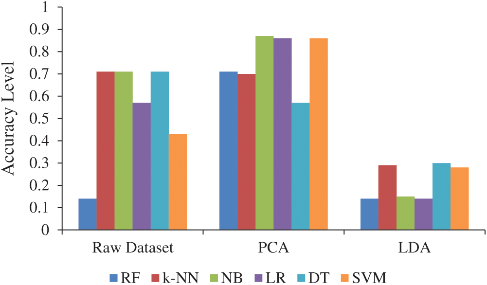
Figure 4: Accuracy level of normalization techniques and raw dataset (Abbreviations: LDA, Linear discriminant analysis; PCA, Principal component analysis; RF, Random forest; k-NN, k-nearest neighbors; NB, Naïve Bayes; LR, Logistic regression; DT, Decision tree; SVM, Support vector machine)
The order of importance of the new dataset and features is given in Tab. 5. The results were obtained by reordering the features according to their importance and by applying the feature selection techniques to the original dataset.
Table 5: Feature selection techniques and the importance order of features
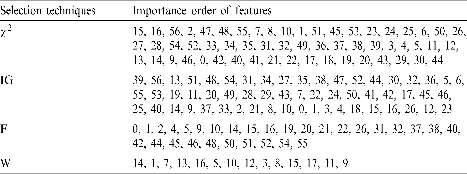
Abbreviations:  , Chi-square; IG, Information gain; F, Forward selection; W, Relief.
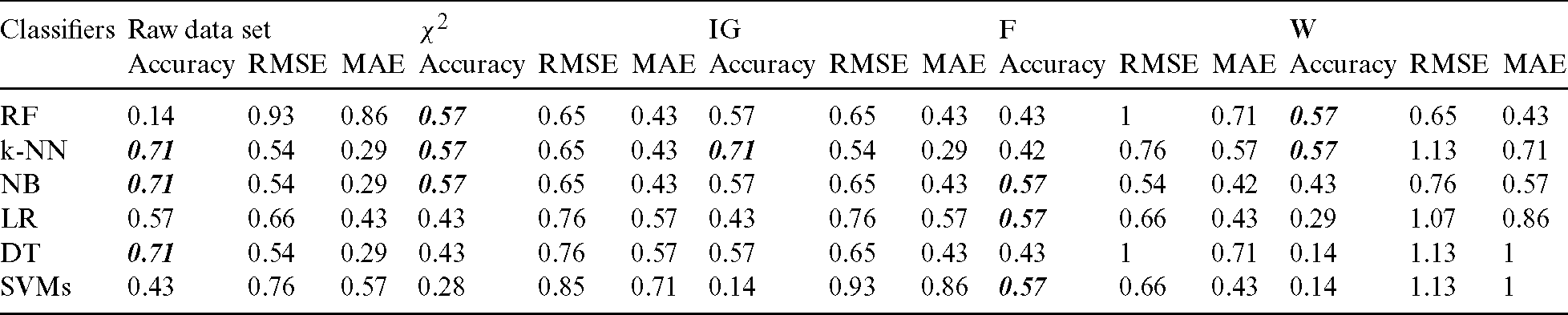
 and IG were used to select and analyze the first 28 features after ranking the importance of features in the dataset. IG performed the best with an accuracy of 0.71 for the k-NN algorithm.
  yielded the best result with an accuracy of 0.57 for RF, k-NN, and NB algorithms (Tab. 6).
Table 6: Accuracy, RMSE, and MAE values of machine-learning classifiers using  , IG, F, and W
Abbreviations:  , Chi-square; IG, Information gain; F, Forward selection; W, Relief; RF, Random forest; k-NN, k-nearest neighbors; NB, Naïve Bayes; LR, Logistic regression; DT, Decision tree; SVMs, Support vector machines; RMSE, Root mean square error; MAE, Mean absolute error.
F ranked the features in the dataset according to their importance and reduced the number to 30 features, which were subsequently used. Similarly, W used 14 features. F with the NB, LR, and SVM algorithms and W with the RF and k-NN algorithms performed the best with an accuracy of 0.57. The accuracy level of the feature selection methods and the raw dataset is given in Fig. 5.
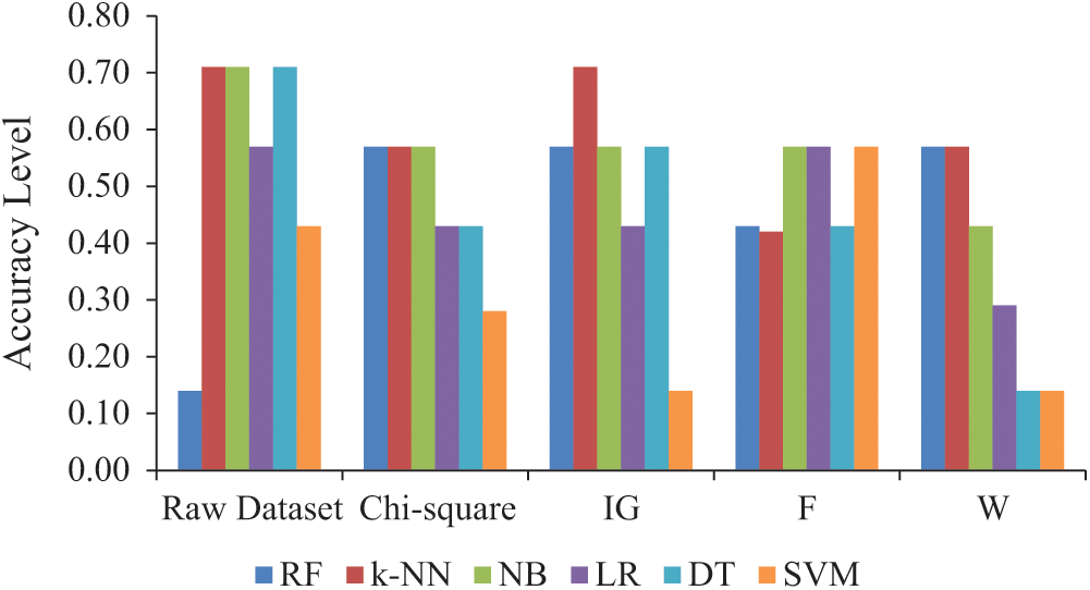
Figure 5: Accuracy level of dimensional reduction methods and raw dataset (Abbreviations: IG, Information gain; F, Forward selection; W, Relief; RF, Random forest; k-NN, k-nearest neighbors; NB, Naïve Bayes; LR, Logistic regression; DT, Decision tree; SVM, Support vector machine)
It is known that most of the exhaustive search and sequential search methods on high-dimensional datasets are not possible with feature selection. Such features that appear important in training data may not provide such good results for test data [21]. In this study, the best accuracy value was found for the k-NN algorithm with IG, namely, an accuracy value of 0.71. This value is equal to the value obtained with the raw data. The study results for feature selection are consistent with the results of Bhaskar et al. [21]. The processing load for feature selection methods can be reduced by selecting the feature that can be used in classification. In this way, the processing time can be shortened. However, the classification accuracy must be acceptable for this to work.
k-NN, NB, and DT algorithms performed effectively for classification tasks in our study. However, the performance of the RF algorithm was not at the desired level. The most successful pre-processing methods in terms of the performance of classification algorithms on LCDS were as follows: (1) Z-score for normalization methods, (2) principal component analysis (PCA) for dimensionality reduction methods, and (3) information gain for feature selection methods. However, selected feature selection methods did not give acceptable levels of accuracy. The ability to effectively diagnose lung cancer was increased with machine-learning methods according to the findings derived from this study. Our study provides evidence that the proposed diagnosis framework has significant potential for the treatment of lung cancer patients and it may assist oncologists by providing early intervention and early diagnosis. The effectiveness of novel machine-learning approaches demonstrated in this study also motivates new research that will focus on computer-aided learning methods for medical applications.
Acknowledgement: I would like to thank Öznur Kol for her support during the study. We also thank LetPub (www.letpub.com) for its linguistic assistance during the preparation of this manuscript.
Funding Statement: This study was funded by TÜBİTAK (The Scientific and Technological Research Council of Turkey) (https://www.tubitak.gov.tr/tr/burslar/lisans/burs-programlari/icerik-2209-a-universite-ogrencileri-arastirma-projeleri-destekleme-programi). The grant name and number are “Machine Learning-Based Lung Cancer Detection” and “2209/A-2018”, respectively.
Conflicts of Interest: The author declares that she has no conflicts of interest to report regarding the present study.
1. World Health Organization (WHO). (2018). “Cancer,” . [Online]. Available: https://www.who.int/en/news-room/fact-sheets/detail/cancer. [Google Scholar]
2. J. Amin, M. Sharif, M. Raza, T. Saba and M. A. Anjum. (2019). “Brain tumor detection using statistical and machine learning method,” Computer Methods and Programs in Biomedicine, vol. 177, pp. 69–79. [Google Scholar]
3. A. M. Salem. (2013). “Advances in intelligent analysis of medical data and decision support systems,” in Machine Learning Applications in Cancer Informatics. Berlin, Germany: Springer, pp. 1–14. [Google Scholar]
4. Y. Gültepe and N. Gültepe. (2020). “Preliminary study for the evaluation of the hematological blood parameters of seabream with machine learning classification methods,” The Israeli Journal of Aquaculture-Bamidgeh, vol. 72, pp. 1–10. [Google Scholar]
5. S. Marsland. (2009). Machine Learning: An Algorithmic Perspective, ed., Boca Raton, Florida, USA: Chapman & Hall/CRC. [Google Scholar]
6. P. G. Espejo, S. Ventura and F. Herrera. (2010). “A survey on the application of genetic programming to classification,” IEEE Transactions on Systems, Man, and Cybernetics—Part C: Applications and Reviews, vol. 40, no. 2, pp. 121–144. [Google Scholar]
7. C. F. Aliferis, I. Tsamardinos, P. P. Massion, A. Statnikov, N. Fananapazir et al. (2003). , “Machine learning on machine learning models for classification of lung cancer and selection of genomic markers using array gene expression data,” in The Sixteenth Int. Florida Artificial Intelligence Research Society Conf., St. Augustine, Florida, United States, pp. 67–71. [Google Scholar]
8. C. M. Lynch, B. Abdollahi, J. D. Fuqua, R. D. De Carlo, J. A. Bartholomai et al. (2017). , “Prediction of lung cancer patient survival via supervised machine learning classification techniques,” International Journal of Medical Informatics, vol. 108, pp. 1–8. [Google Scholar]
9. S. Misra, H. Li and J. He. (2020). “Robust geomechanical characterization by analyzing the performance of shallow-learning regression methods using unsupervised clustering methods,” in Machine Learning for Subsurface Characterization. Oxford, United Kingdom: Gulf Professional Publishing, pp. 129–155. [Google Scholar]
10. C. Nantasenamt, C. Isarankura-Na-Ayudhya, T. Naenna and V. Prachayasittikul. (2020). “A practical overview of quantitative structure-activity relationship,” EXCLI Journal, vol. 8, pp. 74–88. [Google Scholar]
11. T. Jayalakshmi and A. Santhakumaran. (2011). “Statistical normalization and back propagation for classification,” International Journal of Computer Theory and Engineering, vol. 3, no. 1, pp. 1793–8201. [Google Scholar]
12. S. Karasu, R. Hacıoğlu and A. Altan. (2018). “Prediction of Bitcoin prices with machine learning methods using time series data,” in 26th Signal Processing and Communications Applications Conf., Çesme, İzmir, Turkey. [Google Scholar]
13. W. Wang and Z. Xu. (2004). “A heuristic training for support vector regression,” Neurocomputing, vol. 61, no. 1, pp. 259–275. [Google Scholar]
14. O. C. Hamsici and A. M. Matinez. (2008). “Bayes optimality in linear discriminant analysis,” IEEE Transactions on Pattern Analysis and Machine Intelligence, vol. 30, no. 4, pp. 647–757. [Google Scholar]
15. M. Martinez and A. C. Kak. (2001). “PCA versus LDA,” IEEE Transactions on Pattern Analysis and Machine Intelligence, vol. 23, no. 2, pp. 228–233. [Google Scholar]
16. C. Jie, L. Jiawei, W. Shulin and Y. Sheng. (2017). “Feature selection in machine learning: A new perspective,” Neurocomputing, vol. 300, pp. 70–79. [Google Scholar]
17. Y. Gültepe. (2019). “A comparative assessment on air pollution estimation by machine learning algorithms,” European Journal of Science and Technology, no. 16, pp. 8–15. [Google Scholar]
18. C. F. Aliferis, D. P. Hardin and P. P. Massion. (2002). “Machine learning models for lung cancer classification using array comparative genomic hybridization,” in Proc AMIA Sym., San Antonio, Texas, USA, pp. 7–11. [Google Scholar]
19. Lung Cancer Dataset. (2019). “UCI Machine Learning Repository,” Irvine, CA: University of California, School of Information and Computer Science. [Google Scholar]
20. X. Wang and K. K. Paliwal. (2003). “Feature extraction and dimensionality reduction algorithms and their applications in vowel recognition,” Pattern Recognition, vol. 36, no. 10, pp. 2429–2439. [Google Scholar]
21. H. Bhaskar, D. C. Hoyle and S. Singh. (2006). “Machine learning in bioinformatics: A brief survey and recommendations for practitioners,” Computers in Biology and Medicine, vol. 36, no. 10, pp. 1104–1125. [Google Scholar]
22. X. Jin, A. Xu, T. Bie and P. Guo. (2006). “Machine learning techniques and chi-square feature selection for cancer classification using sage gene expression profiles,” Data Mining for Biomedical Applications, vol. 3916, pp. 106–115. [Google Scholar]
23. B. Azhagusundari and A. S. Thanamani. (2013). “Feature selection based on information gain,” International Journal of Innovative Technology and Exploring Engineering, vol. 2, no. 2, pp. 18–21. [Google Scholar]
24. J. L. Bouchot, G. Ditzler, S. Essinger, Y. Lan, G. Rosen et al. (2013). , “Advances in Machine learning for processing and comparison of metagenomic data,” Computational Systems Biology: From Molecular Mechanisms to Disease, pp. 295–329. [Google Scholar]
25. R. J. Urbanowicz, M. Meeker, W. L. Cava, R. S. Olson and J. H. Moore. (2017). “Relief-based feature selection: Introduction and review,” Journal of Biomedical Informatics, vol. 85, pp. 189–203. [Google Scholar]
26. C. Chen, J. Twycross and J. M. Garibaldi. (2017). “A new accuracy measure based on bounded relative error for time series forecasting,” PLoS One, vol. 12, no. 3, pp. 1–23. [Google Scholar]
27. K. Kourou, T. B. Exarchos, K. P. Exarchos, M. V. Karamouzis and D. I. Fotiadis. (2015). “Machine learning applications in cancer prognosis and prediction,” Computational and Structural Biotechnology Journal, vol. 13, pp. 8–17. [Google Scholar]
28. P. Ramasamy and P. Kandhasamy. (2018). “Effect of intuitionistic fuzzy normalization in microarray gene selection,” Turkish Journal of Electrical Engineering & Computer Sciences, vol. 26, pp. 1141–1152. [Google Scholar]
29. A. Jamal, A. Handayani, A. A. Septiandri, E. Ripmiatin and Y. Effendi. (2018). “Dimensionality reduction using PCA and K-Means clustering for breast cancer prediction,” Lontar Komputer, vol. 9, no. 3, pp. 192–201. [Google Scholar]
30. H. Dhahri, E. A. Maghayreh, A. Mahmood, W. Elkilani and M. F. Nagi. (2019). “Automated breast cancer diagnosis based on machine learning algorithms,” Journal of Healthcare Engineering, vol. 2019, pp. 1–11. [Google Scholar]
31. P. Ferroni, F. M. Zanzotto, S. Riondino, N. Scarpato, F. Guadagni et al. (2019). , “Breast cancer prognosis using a machine learning approach,” Cancers, vol. 11, no. 3, pp. 328. [Google Scholar]
32. J. Taninaga, Y. Nishiyama, K. Fujibayashi, T. Gunji, N. Sasabe et al. (2019). , “Prediction of future gastric cancer risk using a machine learning algorithm and comprehensive medical check-up data: A case-control study,” Scientific Reports, vol. 9, 12384. [Google Scholar]
33. A. Sharma and R. Rani. (2019). “C-HMOSHSSA: Gene selection for cancer classification using multi-objective meta-heuristic and machine learning methods,” Computer Methods and Programs in Biomedicine, vol. 178, pp. 219–235. [Google Scholar]
34. X. Dai, I. Spasić, B. Meyer, S. Chapman and F. Andres. (2019). “Machine learning on mobile: An on-device inference app for skin cancer detection,” in Fourth Int. Conf. on Fog and Mobile Edge Computing, Rome, Italy, pp. 301–305. [Google Scholar]
35. J. Lu, E. Song, A. Ghoneim and M. Alrashoud. (2020). “Machine learning for assisting cervical cancer diagnosis: An ensemble approach,” Future Generation Computer Systems, vol. 106, pp. 199–205. [Google Scholar]
36. M. Sinkala, N. Mulder and D. Martin. (2020). “Machine learning and network analyses reveal disease subtypes of pancreatic cancer and their molecular characteristics,” Scientific Reports, vol. 10, pp. 1212. [Google Scholar]
37. S. Goldenberg, G. Nir and S. E. Salcudean. (2019). “A new era: Artificial intelligence and machine learning in prostate cancer,” Nature Reviews Urology, vol. 16, pp. 391–403. [Google Scholar]
38. R. Cuocolo, M. B. Cipullo, A. Stanzione, L. Ugga, V. Romeo et al. (2019). , “Machine learning applications in prostate cancer magnetic resonance imaging,” European Radiology Experimental, vol. 3, pp. 35. [Google Scholar]
39. G. Cammarota, G. Ianiro, A. Ahern, C. Carbone, A. Temko et al. (2020). , “Gut microbiome, big data and machine learning to promote precision medicine for cancer,” Nature Reviews Gastroenterology & Hepatology, vol. 17, pp. 635–648. [Google Scholar]
40. R. Sujitha and V. Seenivasagam. (2020). “Classification of lung cancer stages with machine learning over big data healthcare framework,” Journal of Ambient Intelligence and Humanized Computing. [Google Scholar]
41. S. Jain, S. Shukla and R. Wadhvani. (2018). “Dynamic selection of normalization techniques using data complexity measures,” Expert Systems with Applications, vol. 106, pp. 252–262. [Google Scholar]
42. E. Lotfi and A. Keshavarz. (2014). “Gene expression microarray classification using PCA–BEL,” Computers in Biology and Medicine, vol. 54, pp. 180–187. [Google Scholar]
43. M. Naseriparsa and M. M. R. Kashani. (2013). “Combination of PCA with SMOTE resampling to boost the prediction rate in lung cancer dataset,” International Journal of Computer Applications, vol. 77, no. 3, pp. 33–38. [Google Scholar]
 | This work is licensed under a Creative Commons Attribution 4.0 International License, which permits unrestricted use, distribution, and reproduction in any medium, provided the original work is properly cited. |