DOI:10.32604/cmc.2021.014191
| Computers, Materials & Continua DOI:10.32604/cmc.2021.014191 | |
| Article |
Optimality of Solution with Numerical Investigation for Coronavirus Epidemic Model
1Department of Mathematics and Statistics, The University of Lahore, Lahore, Pakistan
2Department of Mathematics, University of Management and Technology, Lahore, Pakistan
3Department of Mathematics, Cankaya University, Balgat, Ankara, 06530, Turkey
4Department of Medical Research, China Medical University Hospital, China Medical University, Taichung, Taiwan
5Institute of Space Sciences, Magurele-Bucharest, Romania
6Department of Mathematics, Lahore College for Women University, Lahore, Pakistan
7Department of Mathematics, National College of Business Administration and Economics Lahore, Pakistan
8Department of Mathematics, Faculty of Sciences, University of Central Punjab, Lahore, Pakistan
*Corresponding Author: Ali Raza. Email: Alimustasamcheema@gmail.com
Received: 04 September 2020; Accepted: 01 December 2020
Abstract: The novel coronavirus disease, coined as COVID-19, is a murderous and infectious disease initiated from Wuhan, China. This killer disease has taken a large number of lives around the world and its dynamics could not be controlled so far. In this article, the spatio-temporal compartmental epidemic model of the novel disease with advection and diffusion process is projected and analyzed. To counteract these types of diseases or restrict their spread, mankind depends upon mathematical modeling and medicine to reduce, alleviate, and anticipate the behavior of disease dynamics. The existence and uniqueness of the solution for the proposed system are investigated. Also, the solution to the considered system is made possible in a well-known functions space. For this purpose, a Banach space of function is chosen and the solutions are optimized in the closed and convex subset of the space. The essential explicit estimates for the solutions are investigated for the associated auxiliary data. The numerical solution and its analysis are the crux of this study. Moreover, the consistency, stability, and positivity are the indispensable and core properties of the compartmental models that a numerical design must possess. To this end, a nonstandard finite difference numerical scheme is developed to find the numerical solutions which preserve the structural properties of the continuous system. The M-matrix theory is applied to prove the positivity of the design. The results for the consistency and stability of the design are also presented in this study. The plausibility of the projected scheme is indicated by an appropriate example. Computer simulations are also exhibited to conclude the results.
Keywords: Spatio-temporal; advection; diffusion; explicit estimates; auxiliary data; M-matrix
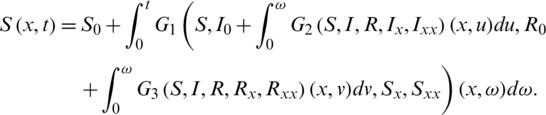
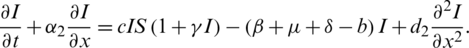
Transmission of different infectious diseases occur in various parts of the world. To understand the dynamics of these, mathematicians have developed and analysed the mathematical models by taking into account their different aspects [1–7]. These models have a vital role to mitigate and to design the control strategy for the diseases. COVID-19 is one of the infectious diseases which creats severe acute respiratory syndrome. In December 2019, the first case of novel coronavirus was diagnosed in Wuhan, China and now, the whole world is in its deadly grip [8]. World Health Organization (WHO) declared this disease, a pandemic in the first half of 2020 [9]. According to the medical experts, this type of virus is extremely dangerous for old people having problems related to lungs, immune system, diabetes and blood pressure [10]. After the spread of this disease, the confirmed cases increased rapidly because of the non-availability of the vaccine. There may be more reasons for its spread, for instance, lack of awareness, lack of facilities to take the precautionary measures and many more. Due to this situation, the number of deaths are increasing day by day. The health workers including doctors, paramedical and other staff of the local health centers are in a high danger zone. Because, they face the infected people on the front lines. So, the identification of the infected cases is necessary at the initial stage so that the disease could not be transmited to other people. Since the beginning of 2020, a large number of confirmed cases exposed in the other cities of China. Now, it has diffused all over the world. In the middle of April 2020, the virus affected almost all the countries on the globe and 1,929,995 confirmed cases and 119,789 deaths were recorded [11]. There are different thoughts in the world about the dispersion of COVID-19. According to some people, it is transmitted due to bats, and some associate it with the seafood market [12]. Another strong reason for the fast-spreading of this virus is the traveling of infected persons, globally [13,14]. It is considered that COVID-19 is transmitted from animal to human, as most of the initial infected cases in Wuhan suspected that it is due to the seafood and animal market in the city [15]. later, it was noticed that, the virus is transmitting from human to human also [16]. Now, in the current situation, this pandemic has become a great threat for the whole world. It has damaged seriously, the life of humans. Since harmful impacts can be seen in the economy, health, education, employment and social life. In order toprovide security, every country is taking some serious steps depending on its available resources. The mathematicians are also observing the dynamics of this disease and trying to describe its behavior by developing the mathematical models. These models are helpful for the policymakers and scientists to understand the disease dynamics. They can make a future prediction of the disease communication and some precautionary measures may be adopted to save the lives of the population. The different aspects of COVID-19 has also attracted the other researchers and they have been studying the disease since a few months [17,18]. After developing a suitable mathematical model of this infection, it is a challenge for the researchers to find the solutions to these models. Usually, these models have a number of parameters (defining the rates with which various compartments are affected) so, in general, it becomes hard to find their analytical solutions. In this situation, the numerical solutions to these models are investigated. Numerical solutions and simulations help us to understand the behavior of the disease, especially when advection and diffusion terms are included in the model. In this article, a Spatio-temporal epidemic model of COVID-19 with advection and diffusion phenomena is analyzed. In the first section, the optimal existence of the solution is discussed and explicit estimates of the solution for the admissible auxiliary data are formulated. In Section 2, the non-standard finite difference (NSFD) method is developed for the proposed model and numerical solutions are found. In Section 3, the important physical properties of our numerical scheme are discussed. The positivity of the proposed scheme is also proved by applying the M-matrix theory. In Section 4, numerical simulations are presented. Concluding remarks are given in the last Section 5. In this article, a Spatio-temporal epidemic model regarding COVID 19 with advection and diffusion is analyzed. The model is described as:

where,  represents the susceptible individuals,
  is identified as infected population,
  is recovered population, a represents the recruitment rate,
  is the natural death rate,
  (death ratedue to corona virus), b (immigration rate of infected population),
  (recovery rate from infection),
  (recovery rate from corona virus), c (infection rate) and
  describes the rate of recovered individuals that lose immunity. Also,
  and
and  represent the advection coefficients while
  stand for diffusion coefficients.
The initial conditions for the system (1) are  ,
,  and
and  .
.
The corona virus free equilibrium for the model (1) is 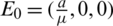 .
.
And, the corona existence equilibrium is
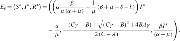
where  ,
,  . The basic reproduction number denoted by
  , is given as
 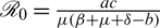 .
.
To examine the epidemic model (system of differential equations) incorporating the advection and diffusion terms, the understanding of the differential equations in epidemic model of the underlying system is necessary. These governing equations make the model easy for studying. To solve these equations for the underlying epidemic model numerically, it is important to investigate the existence, uniqueness, and convergence of the solution to the fixed point or equilibrium point [19,20]. Existence of the solution forthese types of models is mandatory before finding the numerical solution.When the solution of the system is confirmed, then the next task is to find the desirable solutions that can be approximated. Lastly, a most feasible solution is picked out, which is in accordance with the constraints of the system. In general, the solutions to the differential equations lie in the spaces of functions which are known as Banach spaces. Generally, the solutions (functions) to the differential equations are not globally bounded so, it is always better to consider the subset of a function space. The explicit estimates can also be formulated. In 2005, Tutschke introduced the notion of explicit estimates for the general operator equations [21]. Initially, the problems are changed in to the form of fixed-point operators and their solutions are ensured in the subsets of the function spaces that lead to the restriction on the diameter of the subsets for given boundary values or intervals. Similarly, a chosen diameter can also lead to the restriction to the admissible auxiliary data. The subset (closed ball) for which the restriction is imposed, is called optimal ball. In the best of our knowledge, the explicit estimates with the optimal balls for any epidemic model have never been discussed.
In this section, optimal conditions are investigated in the frame work of Banach space, for some related quantities used in the procedure of developing the results, concerning the existence of optimal solutions of the proposed COVID-19 model (1). The system (1) can be reshaped in more general form

In this form G1, G2 and G3 are real valued functions that may be nonlinear, such that the nonlinearity of G1, G2 and G3 may depend not only on S, I and R but also on Sx, Sxx, Ix, Ixx, Rx and Rxx The solutions of above system (2) can be written in the following equivalent form:
After combining these equations, we get,
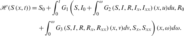
According to the operator theory, the above integral equation which is considered for the solution of (2), can be written in operator form, as

Now, consider the Banach space  , for any
  0. For the existence of the solution of system (1), Shauder fixed point theorem will be used here. For this, it is necessary to prove the fixed-point operator
  to be a self mapping on
  , that is
 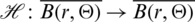 defined by
Suppose also, that  is bounded by
  , that is
 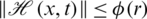 , where
  is a continuous real valued function. Optimization for the proposed model will be done in this space. For this purpose, a closed and convex subset of the Banach space will be chosen which is called a closed ball in X. The consideration of this closed ball yields two cases:
Case 1. Assume that  be a closed ball with center at
  , zero of X, and radius r. Consider,
where,
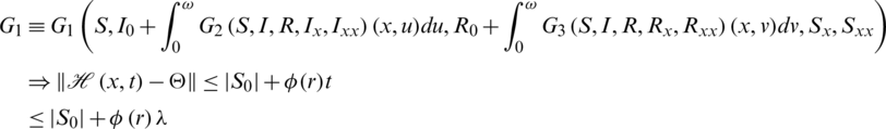
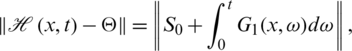
For  to be a self-mapping it should satisfy

The optimized value of r can be obtained by fixing S0 and  , the length of interval of continuity, which is calculated from

Also, by fixing the values of S0 and r, we can optimize  such that

To obtain the greatest value of  , one must have to maximize
  . For this purpose, after some calculations for maximization of a function, we get an equation

Let R* be an optimized radius of the closed ball. Clearly, it will satisfy the Eq. (6).
On the other hand, if we fix  , then from (3) we can optimize the value of S0

Again, the maximum value of  gives the maximum S0. In this case, assume that R* * be the optimized radius which will satisfy the expression
  .
.
Case 2. Assume that  be a closed ball with center at S0, initial condition,and radius r.
Now, consider
where,
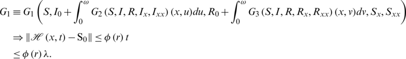
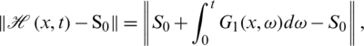
For  to be a self map it should have

The fix values of S0 and  give the optimized radius, such that

Again, for the fixed values of S0 and r, we can optimize  such that

Similarly, to obtain the large interval of continuity, one must have to maximize  , where
  is supposed to be differentiable so, the optimal radius r = R* * should satisfy the equation

If,  is twice differentiable on R then,
  .
.
If,  , for all values of r then,
  will be maximum for every R* *, which is the exact root of (11). According to the theory of calculus, between any two maxima for a function, there exists at least one point at which the function has minimum value. Therefore, with the presence of condition
  , Eq. (11) has not more than one solution. An important result can be developed in the light of above discussion. The following theorem is established in this respect.
Theorem: Suppose that,  be a continuously differentiable function then, the equation
  has a root which becomes an optimal radius. Moreover, for
  and
and  , there exists at most one optimal radius of a closed and convex subset of a Banach space X which possesses the solution of (1). Numerical analysis has a prominent role in the study of applied mathematics, specially for the analysis of epidemic models. To find the solutions of these models, we use different numerical techniques and through simulation we confirm the behavior of the solution. The numerical techniques which preserve the important properties of the model, for instance, positivity, consistency, stability, convergence and boundedness [22–24]. In the next section, a suitable nonstandard finite difference scheme is applied to obtain the numerical solution.
3 Numerical Analysis of Proposed Model
The finite difference methods make, the approximate solutions of the systems involving linear and nonlinear systems of partial differential equations, easy [25]. In these techniques, we convert the continuous model in to a discrete formulation choosing the finite number of function values at some finite number of points in the domain, which is easy to handle. The Taylor’s series is the bestway to obtain these approximations. Now, let M and N be any to finite positive integers and T be any positive real number. The spatial interval  over the time period
  are discretized according to the partitions
  and
and  respectively, with the norm
  and
and  . Divide
  having
  grid points with space and time step sizes h and k respectively. The points of the partitions now become xi = ih and tn = nk, where
  and
and 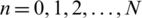 . Suppose that,
  and
and  denote the approximations of S(x, t), I(x, t) and R(x, t) respectively at the grid points
  In this article, we use a non-standard finite difference implicit scheme carrying some important physical properties for the discrete model, developed in [26]. Discrete model equations form a matrix or iterative process that are used to find the best approximation of the solution to the system (1). The system (1) can be converted in to discrete form by using the following approximations.
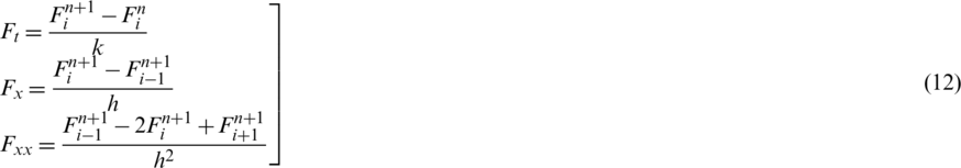
From first Eq. of (1),
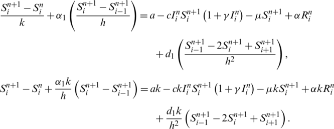
By substitute  ,
,  , we get the expression given below,

Again, second Eq. of (1) becomes as

Put  and
and 

Also, the third Eq. of (1) becomes as follows,

Insert  ,
,  in above, we get

4 Physical Properties of the Proposed Numerical Scheme
4.1 Consistency of the Discrete Model
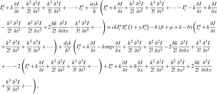
After developing the discrete model from the continuous model, it is very important to check whether the discrete model is consistent with the given continuous model because, the solution of the discrete model approximates the exact solution associated to the continuous model. We also observe the order of consistency of our proposed scheme. After using the approximations (12) and Taylor series in all the equations of (1), we get, first equation of (1)
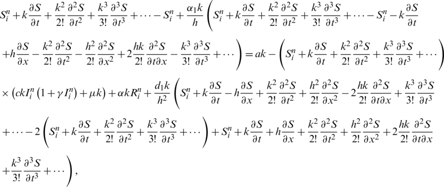
Taking k common from both sides and apply  and
and  we get

From second equation of (1), we get
Taking k common from both sides and apply  and
and  we get
Similarly, we can get third equation of (1). Hence, our proposed scheme is consistent with accuracy of order 2.
4.2 Stability of the Proposed Scheme
From Eq. (13)

After preforming the process of linearization, we get,

Eq. (14) implies
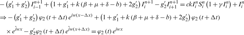
This implies that

Similarly, from Eq. (15), we also have
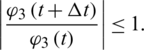
which shows that the proposed scheme is Von-Neumann stable.
According to [27], M-matrix theory is a reliable tool for the verification of the positivity for most of the numerical models concerning engineering, economics, autocatalytic chemical reactions etc. A square matrix over a real field R is said to be an M-matrix if all entries in the off-diagonal are non-positive.
If all the off-diagonal entries of a real matrix A are non-positive then A is called a Z-matrix.
A square matrix A over R is an M-matrix if:
i) A is a Z-matrix.
ii) all the diagonal components of A are positive,
iii) A is strictly diagonally dominant.
It is important to note that M-matrices are non-singular so are invertible and their inverses are positive matrices [28]. This important property will be used in the next result.
Remark: It is clear that M- matrix is a diagonally dominant and its inverse always consists of positive entries.
Theorem: For any  0 and
0 and  0 the discretized system (13)–(15) has positive solutions. That is,
  0,
0,  0 and
0 and  0 for all
  .
.
Proof: It is important to note that the discrete system (13)–(15) generated from finite difference method can be converted in the vector form, such as


In the above setting, D, E, F are square matrices of order (M + 1).
Then

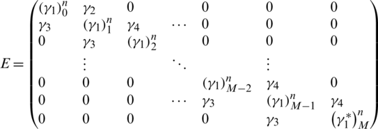

The diagonal elements of  are
are  ,
,  ,
,  and for all
  and the values of off-diagonal elements are
  ,
,  ,
,  .
.
The diagonal elements of  are
are  ,
,  ,
,  and for all
  and the values of off-diagonal elements are
  ,
,  ,
,  .
.
Similarly, the diagonal and off-diagonal entries of  are,
are,  ,
,  ,
,  ; for all
  and
and  ,
,  ,
,  respectively.
The entries in the column matrices of the system (16)–(18) are  ,
,  ,
,  respectively. Also, since
  and
and 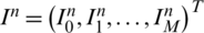 ,
,  and
and  ,
,  and
and  are non-negative so are the diagonal entries of D, E and F. Moreover, all the off-diagonal entries of the matrices D, E, F are negative and the matrices D, E, F are strictly diagonally dominant. This implies that the matrices D, E and F are M-matrices which concludes that D, E and F are non-singular and hence invertible. So (16)–(18) can be written as


Now, suppose that Sn > 0, In > 0 and Rn > 0 and  ,
,  ,
,  satisfy all the conditions on M-matrix which concludes that all the entries of the matrices D−1, E−1, F−1 are positive. So, Sn+1 > 0, In+1 > 0 and Rn+1 > 0. Hence, by induction, the system (16)–(18) has a positive solution. That is, the proposed numerical scheme preserves the positivity of the solution.
5 Numerical Example and Simulations
In this experiment, the following initial conditions are supposed

For the disease free state we take the following values:
a = 0.5,  ,
,  , b = 0.205,
 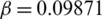 , c = 0.380,
  ,
,  .
.
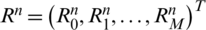
In the Fig. 1, we take the values of parameters in such a way that the value of reproductive number is less than 1. The mesh graphs and combined 2-D plot of all sub-population model are provided in Fig. 1. The SIR corona virus advection diffusion model is manifested two steady states, virus free state and virus existence state. Since in Fig. 1, the value of reproductive number is less than unity therefore model (1) demonstrates the state when virus in not present in the population. Also we see that the state variables present in the system (1) are the population densities. The graphical solutions depicted in the Fig. 1 indicate that the designed technique sustains the positive solution of model (1) and validates the theorem of positivity. Also the stability of virus free steady state of continuous model (1) is retained by designed technique which is again demonstrated in Fig. 1.
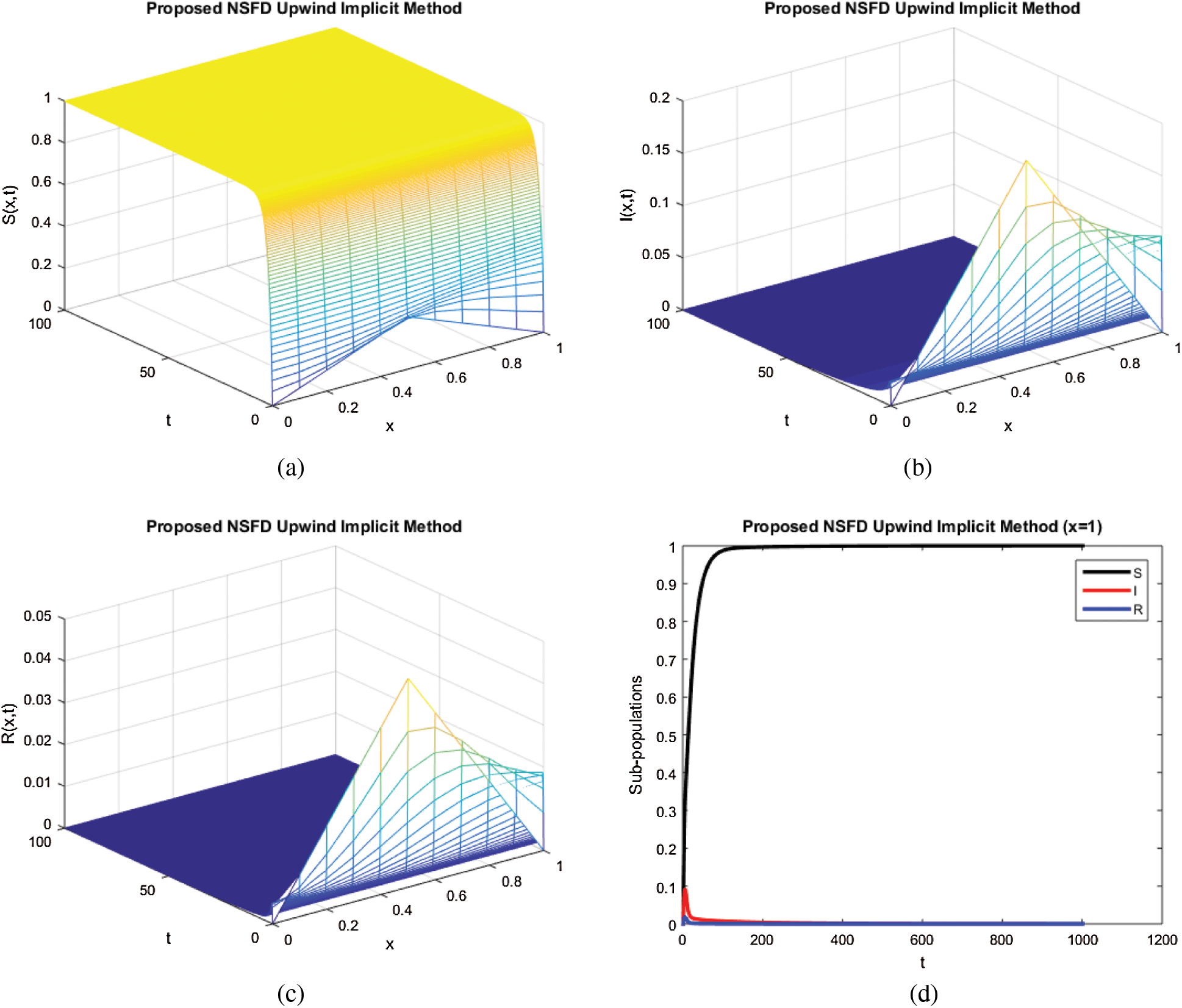
Figure 1: (a) The spatio-temporal simulations results for susceptible population, (b) the spatio-temporal simulations results for infected population, (c) the spatio-temporal simulations results for recovered population, (d) the graphical simulations in 2-D plot for all sub-populations by considering x = 1
For the endemic state we take the following values:
a = 0.5,  ,
,  , b = 0.205,
  , c = 0.580,
  ,
, 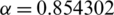 .
.
Fig. 2 indicates the solution mesh graphs and combined two dimensional plot for the steady state at which the virus exists in the population by using proposed technique. Again the positive solution of system (1) is sustained by the upwind NSFD technique. As the values of parameters describe that the value of reproductive quantity is greater than 1, so the corona virus is present in the population and the advection diffusion system (1) possesses the virus persistent in the population. The graphical behavior of all state variables by using proposed technique in the Fig. 2 depicts that the virus is persisted in the population. This shows that the underlying technique is consistent with the continuous model (1).
Figure 2: (a) The spatio-temporal simulations results for susceptible population, (b) the spatio-temporal simulations results for infected population, (c) the spatio-temporal simulations results for recovered population, (d) the graphical simulations in 2-D plot for all sub-populations by considering x = 1
In the current article, we have analyzed a mathematical model concerned with the novel coronavirus disease and the existence and uniqueness of its solution in a closed and convex subset of a banach space is also discussed. The prominent feature of our proposed model is the combination of advection and diffusion in the model which makes the model more realistic and comprehensive. Numerical solution of the proposed model is also computed with the help of nonstandard finite difference scheme which preserves the structural properties of the proposed continuous model. To support the validity of our numerical scheme, we have checked some of its physical properties such as consistency, stability and positivity which is the most important property in any population dynamical model. For positivity, we have used the M-matrix theory. Numerical simulations play a vital role in the study of numerical analysis so, to check the graphical behavior of solution, numerical simulation is also performed that verifies our results. We can extend our work to two and three dimensions.
Funding Statement: The author(s) received no specific funding for this study.
Conflicts of Interest: The authors declare that they have no conflicts of interest to report regarding the present study.
1. C. W. Kanyiri, K. Mark and L. Luboobi. (2018). “Mathematical analysis of influenza: A dynamics in the emergence of drug resistance,” Computational and Mathematical Methods in Medicine, vol. 18, no. 1, pp. 1–14. [Google Scholar]
2. P. Padmanabhan, P. Seshaiyer and C. C. Chavez. (2017). “Mathematical modeling, analysis and simulation of the spread of zika with influence of sexual transmission and preventive measures,” Letters in Biomathematics, vol. 4, no. 1, pp. 148–166. [Google Scholar]
3. C. C. Chavez and B. Song. (2004). “Dynamical models of tuberculosis and their applications,” American Institute of Mathematical Sciences, vol. 1, no. 2, pp. 361–404. [Google Scholar]
4. A. Raza, D. Baleanu, M. Rafiq, M. S. Arif, M. Naveed et al. (2019). , “Competitive numerical analysis for stochastic HIV/AIDS epidemic model in a two-sex population,” IET Systems Biology, vol. 13, no. 6, pp. 305–315. [Google Scholar]
5. K. Abodayeh, A. Raza, M. S. Arif, M. Rafiq, M. Bibi et al. (2020). , “Stochastic numerical analysis for impact of heavy alcohol consumption on transmission dynamics of gonorrhoea epidemic,” Computers, Materials & Continua, vol. 62, no. 3, pp. 1125–1142. [Google Scholar]
6. M. Naveed, D. Baleanu, M. Rafiq, A. Raza, A. H. Soori et al. (2020). , “Dynamical behavior and sensitivity analysis of a delayed coronavirus epidemic model,” Computers, Materials & Continua, vol. 65, no. 1, pp. 225–241. [Google Scholar]
7. W. Gao, P. Veeresha, D. G. Prakasha and H. M. Baskonus. (2020). “Novel dynamic structures of 2019-nCOV with nonlocal operator via powerful computational technique,” Biology, vol. 9, no. 5, pp. 1–19. [Google Scholar]
8. N. S. Goel, S. C. Maitra and E. W. Montroll. (1971). “On the Volterra and other nonlinear models of interacting populations,” Reviews of Modern Physics, vol. 43, no. 2, pp. 1–20. [Google Scholar]
9. T. M. Chen, J. Rui, Q. P. Wang, Z. Y. Zhao, J. A. Cui et al. (2020). , “A mathematical model for simulating the phase based transmissibility of a novel coronavirus,” Infectious Diseases of Poverty, vol. 9, no. 1, pp. 1–8. [Google Scholar]
10. D. S. Hui, E. I. Azhar, T. A. Madani, C. Drosten, A. Zumla et al. (2020). , “The continuing 2019-nCoV epidemic threat of novel coronaviruses to global health the latest 2019 novel coronavirus outbreak in Wuhan China,” International Journal of Infectious Diseases, vol. 91, no. 1, pp. 264–266. [Google Scholar]
11. M. Naveed, M. Rafiq, A. Raza, N. Ahmed, I. Khan et al. (2020). , “Mathematical analysis of novel coronavirus (2019-nCOV) delay pandemic model,” Computers, Materials & Continua, vol. 64, no. 3, pp. 1401–1414. [Google Scholar]
12. A. Atangana. (2020). “Modelling the spread of COVID-19 with new fractal fractional operators: Can the lockdown save mankind before vaccination,” Chaos Solitons and Fractals, vol. 136, no. 1, pp. 1–19. [Google Scholar]
13. Q. Lin, S. Zhao, D. Gao, W. Wang, L. Yang et al. (2020). , “A conceptual model for the coronavirus disease 2019 (COVID-19) outbreak in Wuhan, China with individual reaction and governmental action,” International Journal of Infectious Diseases, vol. 93, no. 1, pp. 211–216. [Google Scholar]
14. M. A. Khan and A. Atangana. (2020). “Modeling the dynamics of novel coronavirus (2019-nCOV) with fractional derivative,” Alexandria Engineering Journal, vol. 59, no. 4, pp. 2379–2389. [Google Scholar]
15. W. Shatanawi, A. Raza, M. S. Arif, K. Abodayeh, M. Rafiq et al. (2021). , “An effective numerical method for the solution of a stochastic coronavirus (2019-nCOVID) pandemic model,” Computers, Materials & Continua, vol. 66, no. 2, pp. 1121–1137. [Google Scholar]
16. A. Raza, M. S. Arif and M. Rafiq. (2019). “A reliable numerical analysis for stochastic gonorrhea epidemic model with treatment effect,” International Journal of Biomathematics, vol. 12, no. 5, pp. 445–465. [Google Scholar]
17. K. Shah, J. Wang, H. Khalil and R. A. Khan. (2018). “Existence and numerical solutions of a coupled system of integral BVP for fractional differential equations,” Advances in Difference Equations, vol. 149, no. 2, pp. 1–19. [Google Scholar]
18. W. Tutschke. (2005). “Optimal balls for the application of the schauder fixed point theorem,” Complex Variables, Theory and Application: An International Journal, vol. 50, no. 1, pp. 697–705. [Google Scholar]
19. N. Ahmed, Z. Wei, D. Baleanu, M. Rafiq and M. A. Rehman. (2019). “Spatiotemporal numerical modeling of reaction-diffusion measles epidemic system,” Chaos: An Interdisciplinary Journal of Nonlinear Science, vol. 12, no. 1, pp. 1–19. [Google Scholar]
20. N. Ahmed, M. Rafiq, M. A. Rehman, M. S. Iqbal and M. Ali. (2019). “Numerical modeling of three dimensional brusselator reaction diffusion system,” AIP Advances, vol. 9, no. 1, pp. 1–18. [Google Scholar]
21. U. Fatima, M. Ali, N. Ahmed and M. Rafiq. (2018). “Numerical modeling of susceptible latent breaking-out quarantine computer virus epidemic dynamics,” Heliyon, vol. 4, no. 5, pp. 1–18. [Google Scholar]
22. D. G. Arson. (1978). “A comparison method for stability analysis of nonlinear parabolic problems,” Society of Industrial and Applied Mathematics, vol. 20, no. 2, pp. 245–264. [Google Scholar]
23. J. W. Bebemes and K. Schmitt. (1979). “On the existence of maximal and minimal solutions for parabolic partial differential equations,” Proceedings of American Mathematical Society, vol. 73, no. 2, pp. 211. [Google Scholar]
24. H. Lin and F. Wang. (2014). “On a reaction–diffusion system modeling the dengue transmission with nonlocal infections and crowding effects,” Applied Mathematics and Computation, vol. 248, no. 1, pp. 184–194. [Google Scholar]
25. B. M. C. Charpentier and H. V. Kojouharov. (2013). “Unconditionally positive preserving scheme for advection diffusion reaction equations,” Mathematical and Computer Modelling, vol. 57, no. 10, pp. 2177–1285. [Google Scholar]
26. R. J. Plemmons. (1977). “M-matrix characterizations nonsingular m-matrices,” Linear Algebra and its Applications, vol. 18, no. 2, pp. 175–188. [Google Scholar]
27. T. Fujimoto, and R. Ranade. (2004). “Two characterizations of inverse-positive matrices: The hawkins-simon condition and the le chatelier-braun principle,” Electronics Journal of Linear Algebra, vol. 1, no. 1, pp. 59–65. [Google Scholar]
28. V. J. Ervin, J. E. Maciyas-Diyaz and J. R. Ramiyrez. (2015). “A positive and bounded finite element approximation of the generalized burgers-huxley equation,” Journal of Mathematical Analysis and Applications, vol. 424, no. 2, pp. 1143–1160. [Google Scholar]
 | This work is licensed under a Creative Commons Attribution 4.0 International License, which permits unrestricted use, distribution, and reproduction in any medium, provided the original work is properly cited. |