Computers, Materials & Continua DOI:10.32604/cmc.2021.014781
Article

High Order Block Method for Third Order ODEs

A. I. Asnor1, S. A. M. Yatim1, Z. B. Ibrahim2 and N. Zainuddin3

1School of Distance Education, Universiti Sains Malaysia, USM Penang, 11800, Malaysia
2Department of Mathematics, Faculty of Science, Universiti Putra Malaysia, Serdang, Selangor Darul Ehsan, 43400, Malaysia
3Department of Fundamental and Applied Sciences, Universiti Teknologi PETRONAS, Seri Iskandar, Perak Darul Ridzuan, 32610, Malaysia
*Corresponding Author: S. A. M. Yatim. Email: ainor@usm.my
Received: 16 October 2020; Accepted: 28 November 2020

Abstract: Many initial value problems are difficult to be solved using ordinary, explicit step-by-step methods because most of these problems are considered stiff. Certain implicit methods, however, are capable of solving stiff ordinary differential equations (ODEs) usually found in most applied problems. This study aims to develop a new numerical method, namely the high order variable step variable order block backward differentiation formula (VSVO-HOBBDF) for the main purpose of approximating the solutions of third order ODEs. The computational work of the VSVO-HOBBDF method was carried out using the strategy of varying the step size and order in a single code. The order of the proposed method was then discussed in detail. The advancement of this strategy is intended to enhance the efficiency of the proposed method to approximate solutions effectively. In order to confirm the efficiency of the VSVO-HOBBDF method over the two ODE solvers in MATLAB, particularly ode15s and ode23s, a numerical experiment was conducted on a set of stiff problems. The numerical results prove that for this particular set of problem, the use of the proposed method is more efficient than the comparable methods. VSVO-HOBBDF method is thus recommended as a reliable alternative solver for the third order ODEs.

Keywords: Block method; stiff ODEs; third order; variable step variable order

1  Introduction

Differential equations are among the most important mathematical tools used in producing models in fields such as the physical sciences, engineering, and biological sciences. In general, the ordinary differential equation (ODE) is an equation that consists of a function and one or more derivatives. A function that satisfies the differential equation is a solution of a differential equation when the function and its derivatives are substituted in the equation. The real-life problems found in science and engineering can be converted into mathematical models in the form of lower or higher order ODEs. The problem of higher order ODEs to be considered in this paper is the third-order stiff ODEs,

with its initial conditions , , , where a and z are finite that represent the starting point and the endpoint respectively.

Some difficult problems may need a solver that can approximate their solutions since these problems may not have actual solutions. In fact, the actual solutions of complex problems are impossible to find. These problems can instead be solved using numerical methods that are tailored to specific cases. There are two important cases that need to be assured in ODEs, particularly stiff or non-stiff cases. Only certain numerical methods can provide suitable solvers for stiff or non-stiff problems. The problems are stiff if they satisfy the following conditions [1],

 i)  , and

ii)   where are the eigenvalues of the Jacobian matrix, and the ratio is called the stiffness ratio of stiffness index.

Unlike non-stiff problems, stiff problems require an implicit method in finding the approximate solutions because the explicit method cannot handle this kind of problems effectively since a very small value of step size is needed. Currently, block backward differentiation formula (BBDF) method is perceived as another solver for stiff ODEs. This method is known to perform better than the non-block backward differentiation formula (BDF) method and MATLAB’s ODE solver [2–4]. BBDF method can produce better approximate solutions and provide numerous solutions simultaneously. By providing numerous solutions simultaneously, the method can significantly reduce computational effort and cost.

In addition to producing numerous solutions simultaneously, BBDF method also requires less computational effort as it is capable of solving higher order problems directly. BBDF method can directly solve higher order problems because it does not require a reduction process to reduce the higher order problems to their first order system before the computational work can start. This will automatically reduce the computational cost, especially in terms of time and the number of total steps taken. The effectiveness of BBDF method in solving higher order problems have been proven in a number of research [5–9]. Albeit implementing different approaches to BBDF method such as constant step size, variable step size, variable order with constant step size in a single code and also variable order with variable step size in a single code for the direct solutions of second order ODEs, these researches have all favoured the method for its effectiveness.

The evolution of various numerical methods in the literature is intended to improve the existing methods by offering better solutions. However, there is a dearth of research in methods that solve higher-order stiff ODEs, especially third-order stiff ODEs. Most past research focused on the special and non-stiff third order ODEs as discussed in [10–13]. We, therefore, aim to develop an efficient direct method to provide numerical solutions for third-order ODEs.

Inspired by the approach applied in a couple of research [6,7], we intend to adopt the variable step and variable order approach in BBDF method for solving the third order stiff ODEs directly. Choosing a suitable step size is imperative in reducing the computation time and the number of iterations, while changing the order helps in finding the best approximation that will produce better or more accurate results.

2  Development of VSVO-HOBBDF Method

This section will explain the development of the high order variable step variable order block backward differentiation formula (VSVO-HOBBDF). VSVO-HOBBDF method consists of order two, three, and four variable step higher order BBDF (VS-HOBBDF) method of different values of the step size in a single code. The illustration of the variable step BBDF method is shown in Fig. 1.

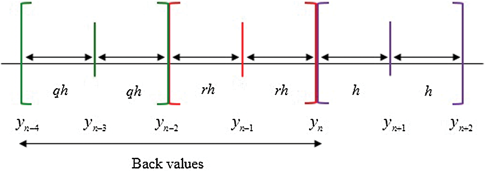
Figure 1: Illustration of variable step BBDF method

h, r, and q in Fig. 1 are defined as step size, step size ratio for the first previous block, and step size ratio for the second previous block respectively. and yn are all the back values while yn+1 and yn+2 are the two new points that we are going to approximate. For each order of the VS-HOBBDF method, the back values will be different. The k back values for each order of the VS-HOBBDF method are specified as follows:

•    Order two VS-HOBBDF (2VS-HOBBDF)

•    Order three VS-HOBBDF (3VS-HOBBDF)

•    Order four VS-HOBBDF (4VS-HOBBDF)

The VS-HOBBDF formulas for order 2, 3, and 4 are derived from Lagrange polynomial. To derive each order of VS-HOBBDF, all the back values and the two new current points will be the interpolation points. We begin the development with 2VS-HOBBDF method.

Development of the First and Second Points of Order Two, Three and Four VS-HOBBDF Method

We begin with the development of 2VS-HOBBDF method as follows:

Step 1:

Taking k = 3 gives the Lagrange polynomial for 2VS-HOBBDF given by

where and .

Step 2:

Replacing in (1) by polynomial (2). Subsequently, referring to Fig. 1, the step size of the computed block is 2h whereas the step sizes for the previous blocks are 2rh and 2qh. Then, substituting them in the polynomials (2) afterward give the polynomials in terms of s, h, and r.

Step 3:

Differentiating the updated polynomials once, twice and thrice with respect to s, then followed by replacing s with 0 at x = xn+1. The polynomials are now in terms of r only.

Step 4:

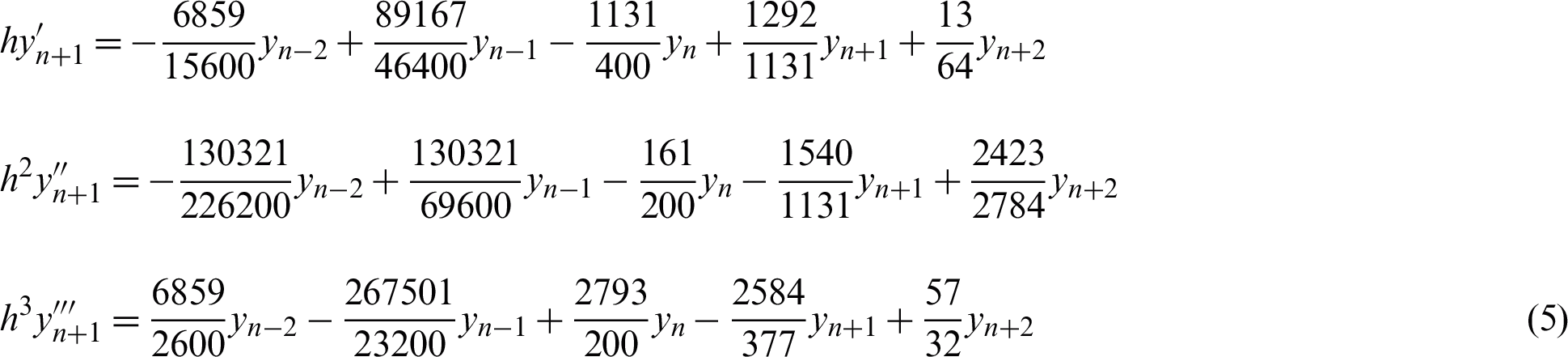
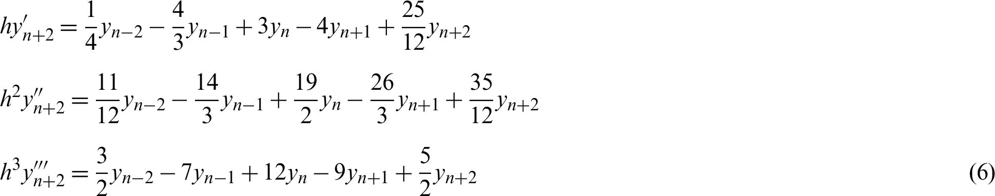
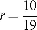
Consequently, replacing r term in first, second and third differentiation with 1, 2 and 10/19 give

r = 1 (Constant step size)

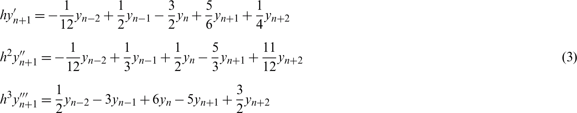
r = 2 (Halving the step size)

(Increment of the step size by a factor of 1.9)

Step 5:

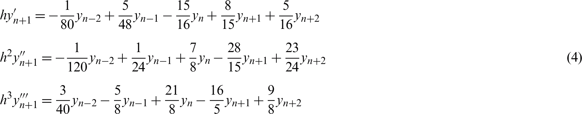
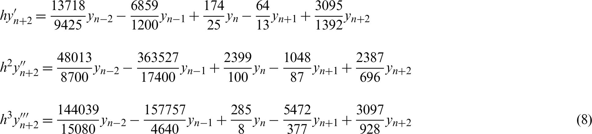
Repeating Step 3 while replacing s with 1 at x = xn+2 and continuing the process with Step 4 to obtain the following equations:

r = 1 (Constant step size)

r = 2 (Halving the step size)

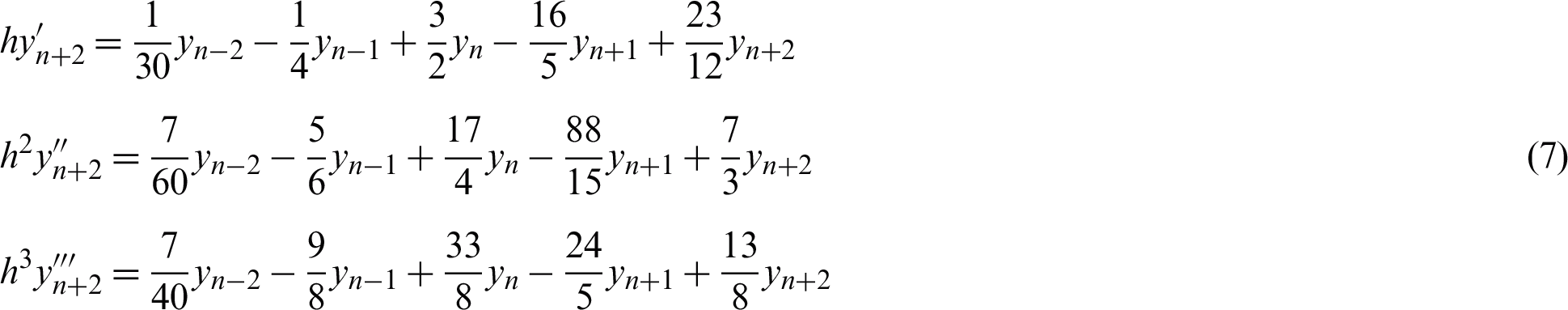
(Increment of the step size by a factor of 1.9)

Step 6:

Repeating Steps 1–5 for deriving the formulae of 3VS-HOBBDF (k = 4) and 4VS-HOBBDF (k = 5) methods.

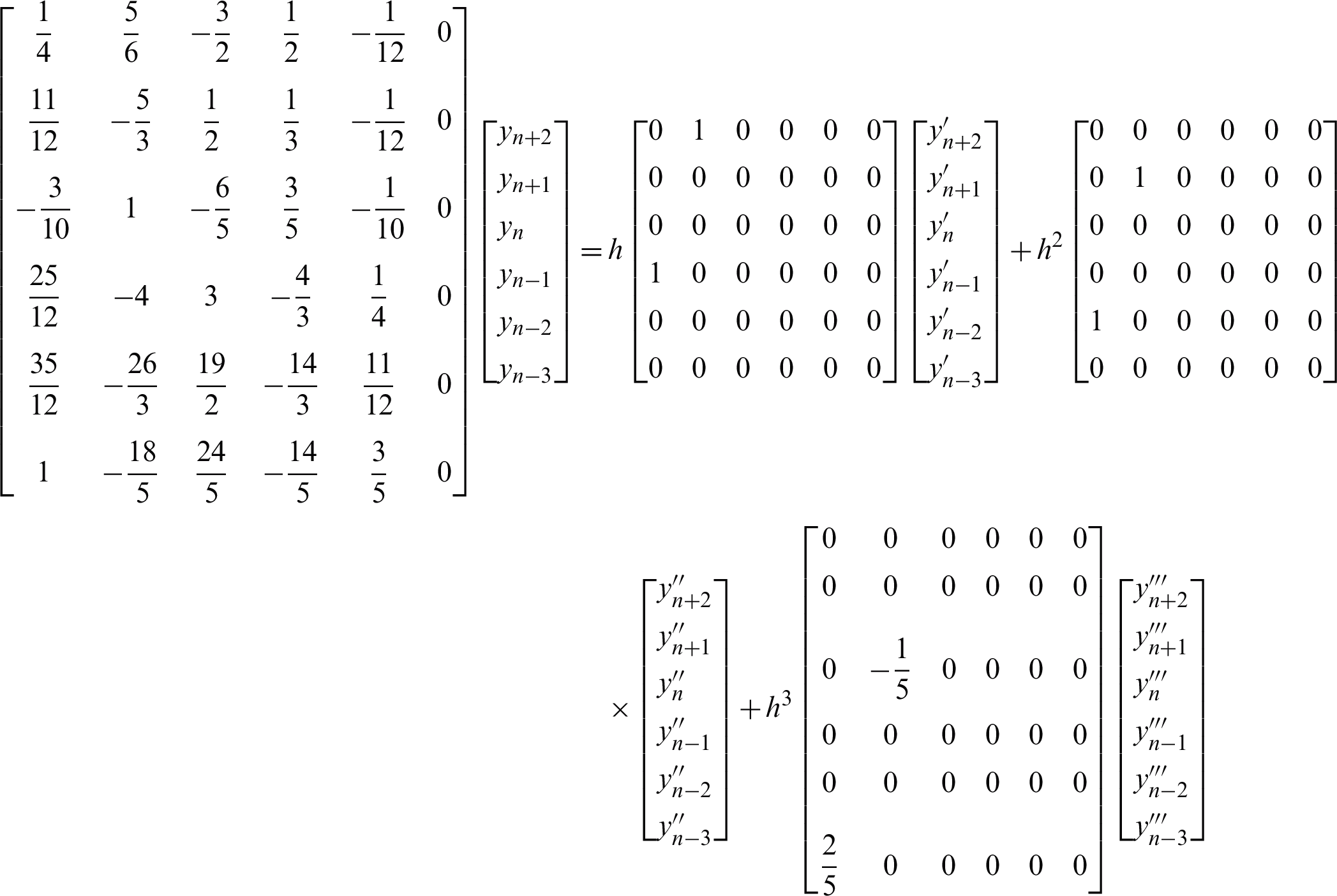
The formulae of VSVO-HOBBDF can be generalised in matrix form as follows:

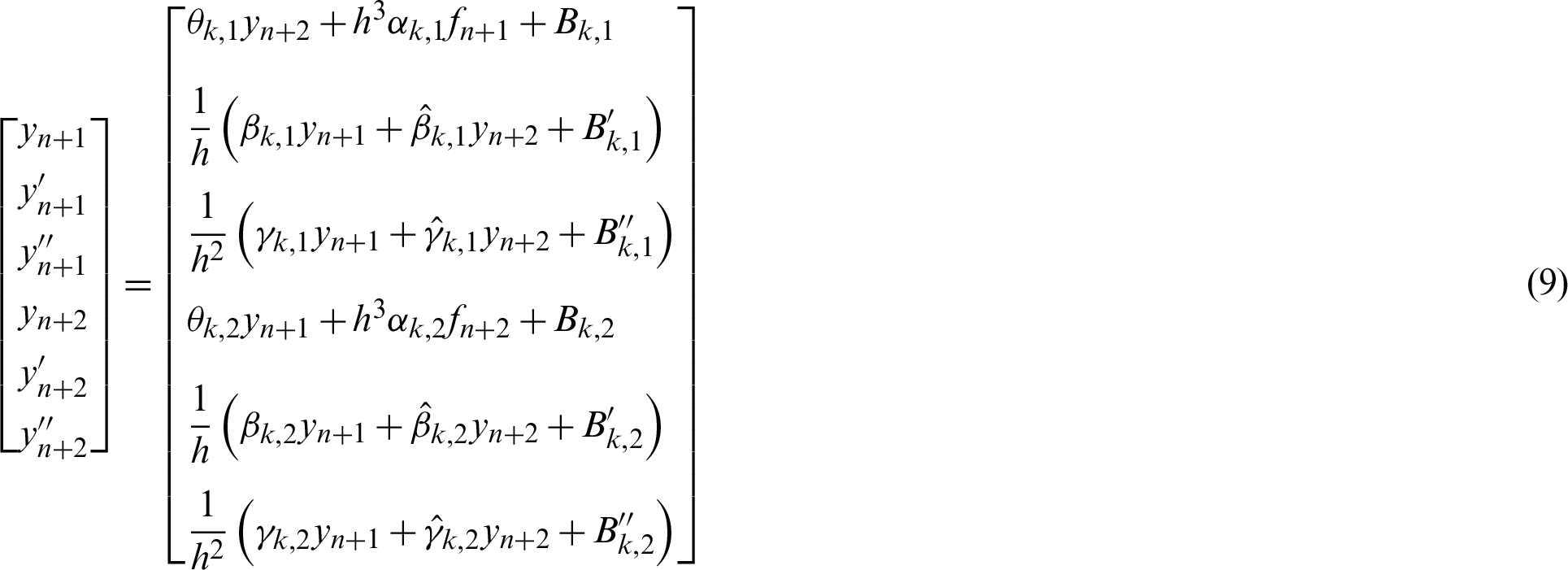
where and are the back values for the first and second point respectively.

3  Implementation of VSVO-HOBBDF Method

This section presents the formulae in the previous section as implemented in two stages of Newton’s iteration. Therefore, the general form of linear equation 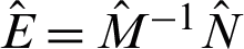is given by

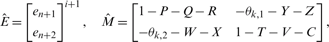
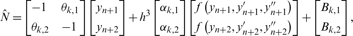
where,

4  Order of VSVO-HOBBDF Method

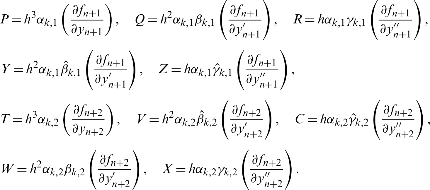
The linear difference operator, associated with the VSVO-HOBBDF method is given by

where is an arbitrary function, continuously differentiable on .

Expanding , , and in (10), as Taylor Series about x. Then, collecting the terms obtain

where coefficients of Cq are constants and assign as follows:

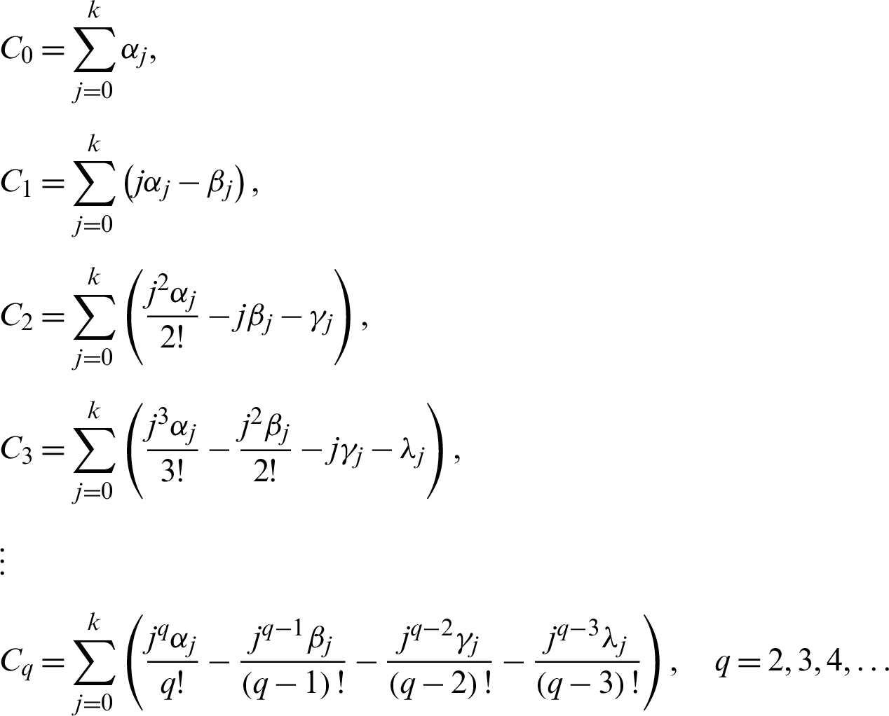
Definition 3

The linear difference operator and the associate LMM in (10) are said to be of order p if and 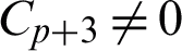. Note that Cp+3 is the error constant.

Applying the following steps to determine the order of each VS-HOBBDF methods by letting the simpler form of the formulae be equivalent to

where , , and are not all zero.

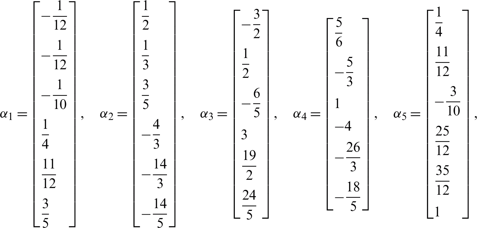
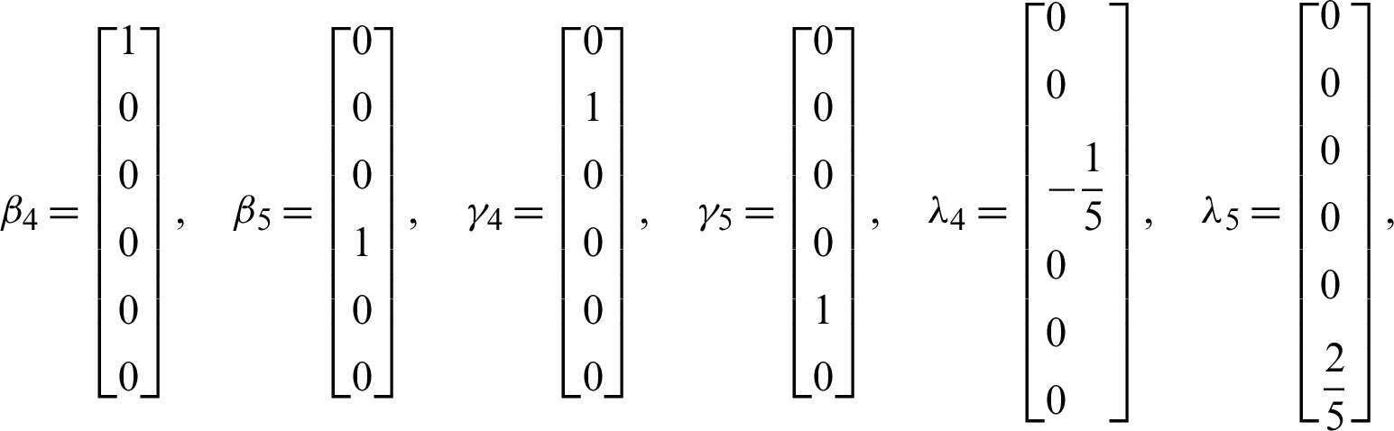
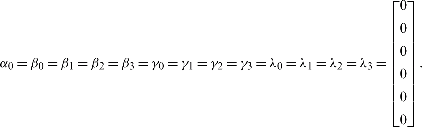
We begin by determining the order of 2VS-HOBBDF method. Rearranging the formulae of 2VS-HOBBDF method in the previous section gives

Subsequently, , , and represent each column of the matrices as follows:

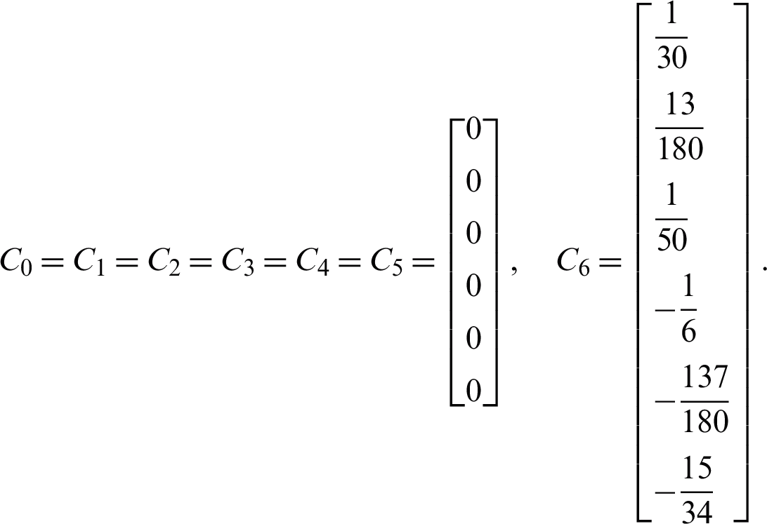
Obtain the values for Cq as follows:

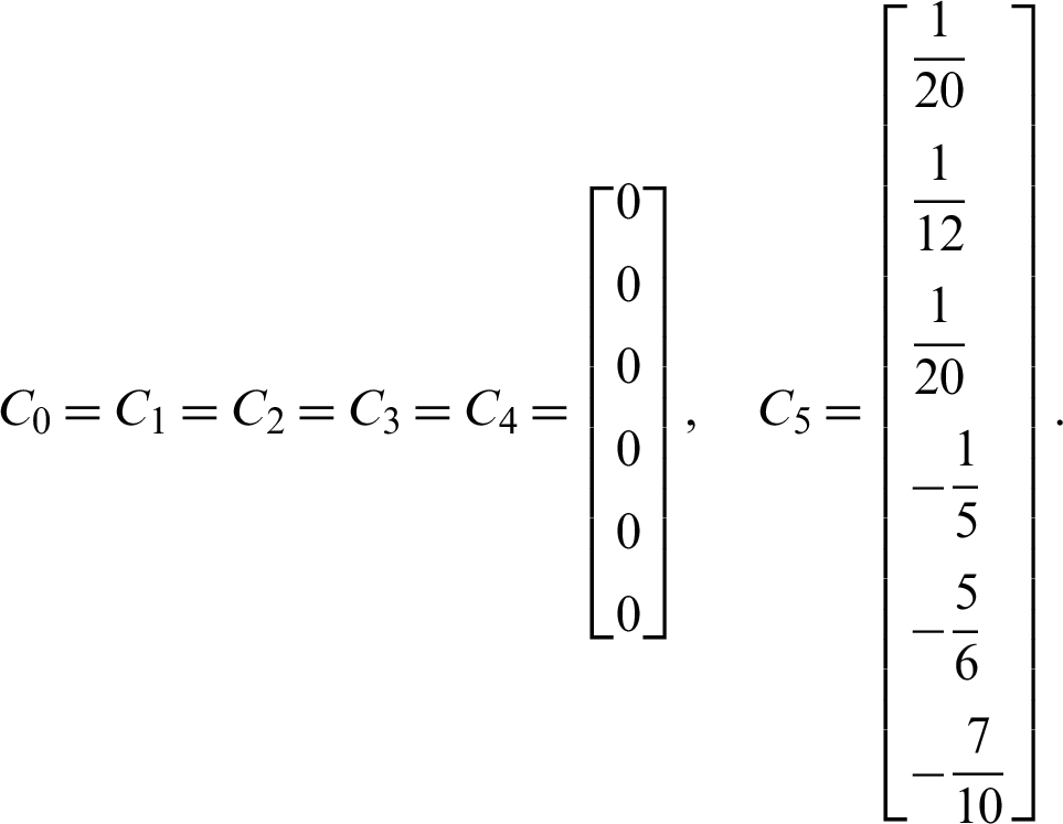
Since , from the Definition 3 gives

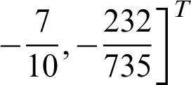
Thereby, the 2VS-HOBBDF is of order two with error constant .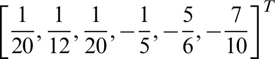

Repeating the similar steps to determine the order of 3VS-HOBBDF and 4VS-HOBBDF methods. The values of Cq for 3VS-HOBBDF and 4VS-HOBBDF methods are obtained as follows:

3VS-HOBBDF

, therefore, the 3VS-HOBBDF is of order three with error constant , .

4VS-HOBBDF

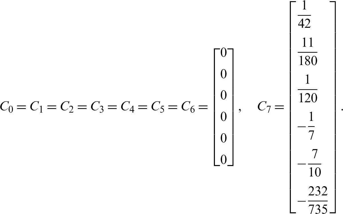
Since , the 4VS-HOBBDF is of order four with error constant , .

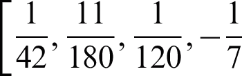5  Technique of Varying the Step Size and Order

The variable step size and variable order approaches are implemented in a single code in the VSVO-HOBBDF method. The order is varied in order to achieve the best solutions with good accuracy while the step size is varied in order to optimize the computational effort.

The technique for varying the step size and order is as follows:

•    Step 1: Start the integration with the 2VS-HOBBDF method.

•    Step 2: Check the local truncation error (LTE)

if (TOL)

Accept the solutions. Go to Step 4.

else

Reject the solutions. Go to Step 3.

Step 3: The step size is halving (r = 2). Repeat the computation for the current block. Go to Step 2.

Step 4: Check the suitable value for the new step size. The new step size is either maintained (r = 1) or increased to a factor of 1.9 (r = 10/19).

Step 5: Proceed with the next block integration step. The order is maintained for two consecutive blocks and is considered to increase the order after two succesful steps.

Step 6: Repeat the Steps 2–5 until the end of the interval.

Note that if two failed steps occurred, the order is decreased.

6  Numerical Experiments

The aim of conducting the numerical experiments was to analyse the performance of the VSVO-HOBBDF method. Three tested problems from the third order ODE were considered for the purpose of testing the proposed method. The performance of the method was tested at different value of tolerances. Note that ode15s is a variable step variable order method based on the numerical differentiation formulas (NDFs) of orders 1 to 5 or backward differentiation formulas (BDFs) and ode23s is based on Modified Rosenbrock formula of order 2.

Problem 1 (Boundary layer flow)

Exact solutions at x = 1 from MATLAB:

ode15s: 0.495900477127

ode23s: 0.495892222080

Problem 2 (Thin film flow)

Exact solutions x = 1 from MATLAB:

ode15s: 2.608276239679

ode23s: 2.608268411808

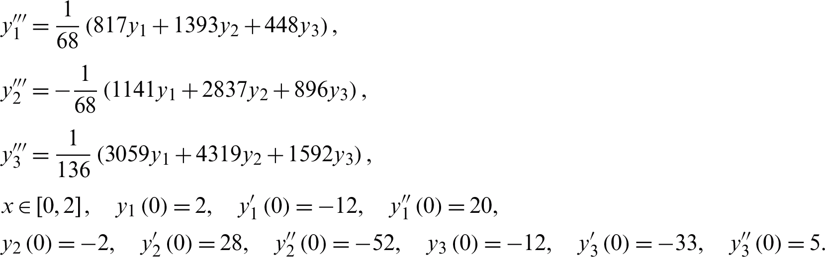
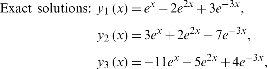
Problem 3 (Linear system)

7  Numerical Results and Discussion

The numerical results were analysed at different value of tolerances, 10−2, 10−3, 10−4, and 10−5. The results obtained from the numerical experiments for all the tested problems are presented in Tabs. 1–3, followed by the analysis of each method’s performance.

Table 1: Numerical results for Problem 1

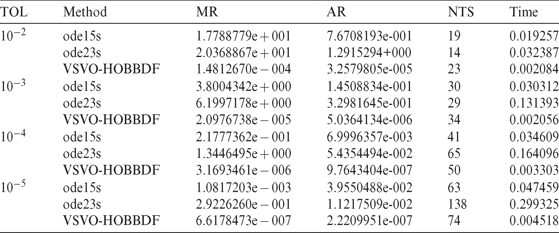
Table 2: Numerical results for Problem 2

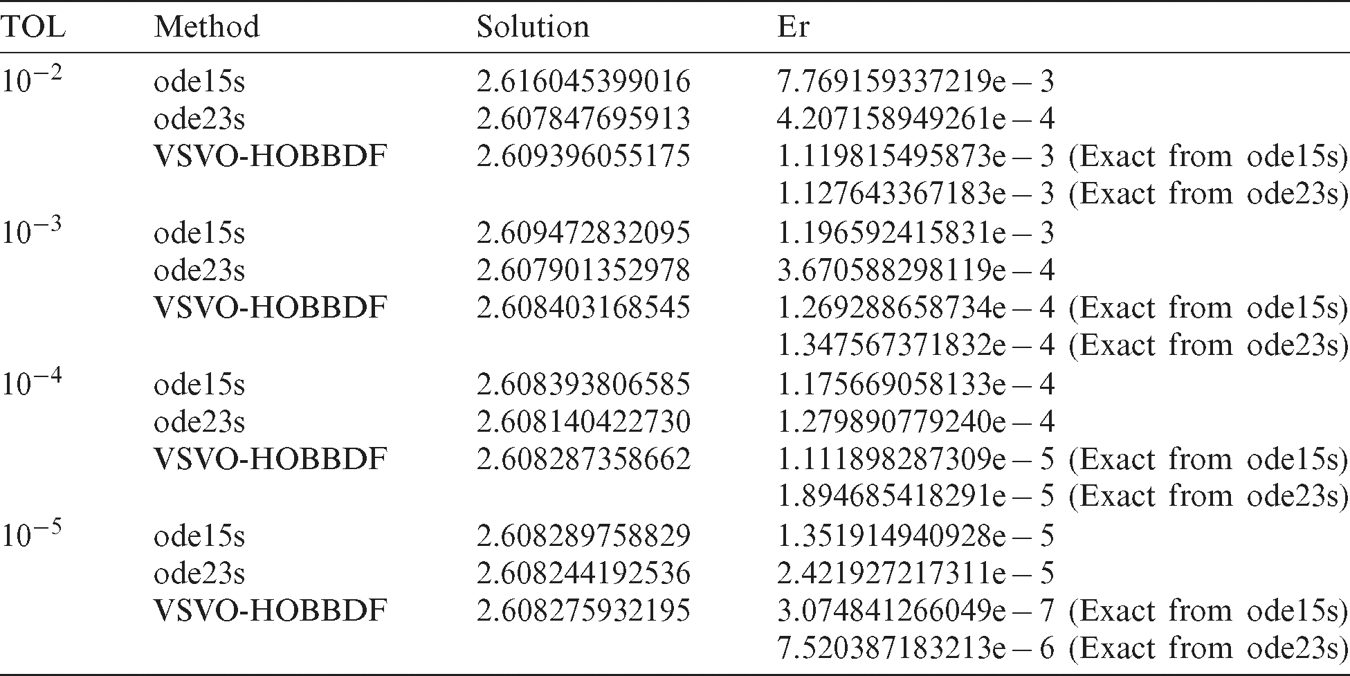
Table 3: Numerical results for Problem 3

On another note, the exact solutions at x = 1 for Problems 1 and 2 are determined by using from ode15s and ode23s in MATLAB since these problems have no exact solutions. Thus, each problem will have two exact solutions.

The error for each integration step is evaluated by letting Er as the error. The average error and maximum error are defined as follows:

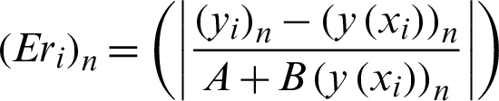
where n is the number of equations, yi is the approximate solutions and are the exact solutions. Mixed error test, A = 1, B = 1 is applied for Problem 3 and A = 1, B = 0, which correspond to the absolute error tests are applied for Problems 1 and 2. For Problems 1 and 2, the Er are calculated at the endpoint, i.e., x = 1.

Meanwhile, the average error (AR) and maximum error (MR) are defined as

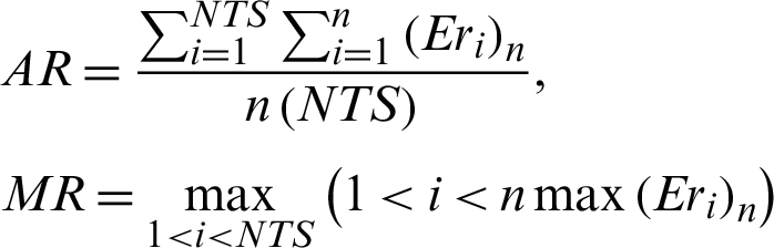
where NTS is the number of total steps.

The numerical results for all the considered problems are presented in Tabs. 1–3. The efficiency of the VSVO-HOBBDF method was analysed at four tolerance values and compared with two MATLAB’s solvers, ode15s and ode23s. As clearly shown, most of the approximated results produced by VSVO-HOBBDF method for Problems 1 and 2 are more accurate, except for Problem 2 at tolerance 10−2 at which ode23s gave better accuracy. The errors produced between the VSVO-HOBBDF method and the exact solutions from ode15s are smaller compared to the errors produced between the VSVO-HOBBDF method and the exact solutions from ode23s. This indicates the VSVO-HOBBDF method is converged to the exact solutions of the ode15s for both problems.

Meanwhile, the approximate solutions of Problem 3 at all tolerance values improved in accuracy when the VSVO-HOBBDF method was applied. From our observation, errors produced by the VSVO-HOBBDF method were smaller as compared to the errors produced by both MATLAB’s codes at all tolerance values. The VSVO-BBDF method also outperformed the ode23s at tolerance values of 10−4 and 10−5 with less number of total steps. As we applied the VSVO-BBDF method to the tested problems, the time taken was also reduced at each tolerance as compared to the MATLAB’s solver.

The results obtained thus proved that the VSVO-BBDF method is effective in solving the considered problems by providing better approximated solutions and reducing the computational cost.

8  Conclusions

This paper delineates an approach by varying the step size and order to the VSVO-HOBBDF method in a single code. The numerical experiments were applied to a number of third-order ODE problems. The performance of VSVO-HOBBDF method was evaluated based on the results. By adapting the variable step size and variable order in the same code, we have proven the efficiency of VSVO-HOBBDF method. The results also suggest that the accuracy is improved and the computational cost is also reduced. Compared to both MATLAB’s codes, VSVO-HOBBDF method performs better and is a reliable direct solver for third order ODEs. Therefore, VSVO-HOBBDF method is recommended as an alternative solver for third-order ODEs.

Funding Statement: This research was funded by Fundamental Research Grant Scheme Universiti Sains Malaysia, Grant No. 203/PJJAUH/6711688 received by S. A. M. Yatim. Url at http://www.research.usm.my/default.asp?tag=3&f=1&k=1.

Conflicts of Interest: The authors declare that they have no conflicts of interest to report regarding the present study.

References

1.  J. D. Lambert. (1991). Stiffness: Linear stability theory in: Numerical Methods for Ordinary Differential Systems: The Initial Value Problem. New York, USA: John Wiley & Sons, pp. 216–217.

2.  Z. B. Ibrahim, K. I. Othman and M. Suleiman. (2007). “Implicit r-point block backward differentiation formula for solving first-order stiff ODEs,” Applied Mathematics & Computation, vol. 186, no. 1, pp. 558–565.

2.  N. A. A. M. Nasir, Z. B. Ibrahim and M. B. Suleiman. (2011). “Fifth order two-point block backward differentiation formulas for solving ordinary differential equations,” Applied Mathematical Sciences, vol. 5, no. 71, pp. 3505–3518.

4.  N. A. A. M. Nasir, Z. B. Ibrahim, K. I. Othman and M. Suleiman. (2012). “Numerical solution of first order stiff ordinary differential equations using fifth order block backward differentiation formulas,” Sains Malaysiana, vol. 41, no. 4, pp. 489–492.

5.  Z. B. Ibrahim, K. I. Othman and M. Suleiman. (2012). “2-point block predictor-corrector of backward differentiation formulas for solving second order ordinary differential equations directly,” Chiang Mai Journal of Science, vol. 39, no. 3, pp. 502–510.

6.  S. A. M. Yatim, Z. B. Ibrahim, K. I. Othman and M. B. Suleiman. (2013). “A numerical algorithm for solving stiff ordinary differential equations,” Mathematical Problems in Engineering, vol. 2013.

7.  S. A. M. Yatim. (2013). “Variable step variable order block backward differentiation formulae for solving stiff ordinary differential equations,” Ph.D. dissertation, Universiti Putra Malaysia, Malaysia.

8.  N. Zainuddin, Z. B. Ibrahim, K. I. Othman and M. B. Suleiman. (2016). “Direct fifth order block backward differentiation formulas for solving second order ordinary differential equations,” Chiang Mai Journal of Science, vol. 43, no. 5, pp. 1171–1181.

This work is licensed under a Creative Commons Attribution 4.0 International License, which permits unrestricted use, distribution, and reproduction in any medium, provided the original work is properly cited.