DOI:10.32604/cmc.2021.014710
| Computers, Materials & Continua DOI:10.32604/cmc.2021.014710 | |
| Article |
COVID-19 and Unemployment: A Novel Bi-Level Optimal Control Model
1Department of Statistics and Operations Research, College of Sciences, King Saud University, Riyadh, Saudi Arabia
2Department of Mathematics, Ibb University, Ibb, Yemen
*Corresponding Author: Ibrahim M. Hezam. Email: ialmishnanah@ksu.edu.sa
Received: 11 October 2020; Accepted: 04 November 2020
Abstract: Since COVID-19 was declared as a pandemic in March 2020, the world’s major preoccupation has been to curb it while preserving the economy and reducing unemployment. This paper uses a novel Bi-Level Dynamic Optimal Control model (BLDOC) to coordinate control between COVID-19 and unemployment. The COVID-19 model is the upper level while the unemployment model is the lower level of the bi-level dynamic optimal control model. The BLDOC model’s main objectives are to minimize the number of individuals infected with COVID-19 and to minimize the unemployed individuals, and at the same time minimizing the cost of the containment strategies. We use the modified approximation Karush–Kuhn–Tucker (KKT) conditions with the Hamiltonian function to handle the bi-level dynamic optimal control model. We consider three control variables: The first control variable relates to government measures to curb the COVID-19 pandemic, i.e., quarantine, social distancing, and personal protection; and the other two control variables relate to government interventions to reduce the unemployment rate, i.e., employment, making individuals qualified, creating new jobs reviving the economy, reducing taxes. We investigate four different cases to verify the effect of control variables. Our results indicate that rather than focusing exclusively on only one problem, we need a balanced trade-off between controlling each.
Keywords: Bi-level optimal control; COVID-19; Hamiltonian function; Karush–Kuhn–Tucker unemployment
The coronavirus disease 2019 (COVID-19) pandemic is likely the biggest contemporary challenge. As the economy enters a long recession, there is an expected corresponding rise in the number of unemployed. Most companies have laid off workers as a precautionary measure and due to the lockdown, which directly spikes up the unemployment rate, while inversely impacting other economic sectors, such as tourism and aviation.
The conflicting goals of controlling COVID-19 and preserving the economy are formidable: stringent measures to control COVID-19 with complete lockdown and social distancing will directly impact business, and firms will have no choice but to lay off workers. Bauer et al. [1] found that unemployment increased by 60% during April 2020 in Germany due to COVID-19 containment measures, which included a complete lockdown. Gong et al. (2020) reviewed the economic impact of COVID-19 and clarified the importance of timely collecting of pandemic information and adopting scientific methods to handle epidemiological information. In addition, the research emphasized upon transparency and the accurate disclosure of information, which, in turn, effectively balances controlling the pandemic and reducing economic losses. They found that economic losses may increase due to the exaggeration of public panic, indifference, and the lack of public awareness. Another important report issued by Legatum Institute [2], in which it showed the economic effects, especially on groups that suffered from poverty before the pandemic, including the disabled people, minorities, those without high qualifications, and in part-time work. The results also showed that the relationship between poverty and the impacts of the COVID-19 is complex driven by overlapping several factors. While Sumner et al. [3] estimated that 5.4%–8% of the world’s population will fall into poverty.
Hence, unemployment is one of the serious challenges contemporarily impacting countries, especially developing nations and unstable economies that are vulnerable to perpetual conflicts and disasters. Consequently, this is one reason for the unemployed persons to be attracted to armed and terrorist groups, coupled with the resultant spreading of crimes and drugs. For this reasons, governments and researchers have given most of their attention to solving the unemployment problem. The mathematicians are contributing to fight this problem through the formulation of some mathematical models and their applications. Mathematical modelling of unemployment has been conducted by several authors [4–10] most such studies classified individuals according to whether the person is unemployed in addition to the class of available vacancies, while also proposing optimal control models. Most of the time-variant variables to control the model varied between government policies to create new jobs along with training the unemployed to become qualified to find jobs and government fiscal policy of employment, economic stimulus, and taxes.
Recently, studies have investigated the COVID-19 epidemiological model including [11–16]. Their models, mathematical analysis, methodology, and data analysis significantly differ. In addition, optimal control models were proffered to curb the COVID-19 outbreak. Suggested measures and interventions included lockdown, isolation, and quarantine, the availability of screening test kits, protection, social distancing, wearing personal protective equipment (PPE) kits, as well as treatment of those infected with COVID-19. Cristina et al. [17] investigated the interaction between COVID-19 and unemployment and found that although full lockdown may reduce the number of infected individuals, it also increases unemployment.
Bi-level optimization is a NP-hard optimization problem, which becomes more complex when the bi-level programming is combined with optimal control models in addition to infinite dimensions. Sinha et al. [18] reviewed the approaches of solving bi-level optimization along with its applications. According to Palagachev [19], the most widely used methods for solving bi-level optimization problems are branch-and-bound, descend, and penalty functions. In addition, the Pontryagin minimum principle and the value function of the follower level are commonly used techniques to solve bi-level optimal control models (BLOC). The authors in [20–23] solved the bi-level optimization using Pontryagin’s maximum principle with an augmented Hamilton function. Palagachev et al. [24] used the value function of the lower level problem. Reference [25] used gradient-based algorithms, while [26] combined indirect and direct approximation method to reduce the bi-level to a single-level problem. References [27–30] used evolutionary techniques to solve inverse optimal control problems. The Karush–Kuhn–Tucker condition was used to reformulate the bi-level to a single level optimal control problem in [31–34].
The current study is characterized by double-sided complexity. First, it investigates the interaction between COVID-19 and the unemployment models. Second, because of the hierarchical structure of bi-level programming and both levels contain infinite dimensions of dynamic partial differential equations, a bi-level optimal control is considered as one of NP-hard optimization.
The contributions of this this paper are five-fold: (1) We formulate a new bi-level dynamic optimization of the interaction between COVD-19 and unemployment. (2) We construct an optimal control model with two objective functions: minimize infected people with COVID-19 and minimize unemployment, while also minimizing the total cost associated with the intervention strategies. (3) The modified approximation KKT and the Hamiltonian function, derived from the Lagrangian function, will deal with the lower level. (4) We investigate the sensitivity of three inputs of the optimal control by evaluating a set of control strategies. The three inputs related to government measures for fighting COVID-19 and government policy for employment and creating new jobs. These three actions are expected to be effective for identifying optimal strategies to balance between COVID-19 control and reducing unemployment. Last, all strategies are conducted in Yemen. Briefly, the presented work is aimed to design an interactive mathematical framework linking COVID-19 with unemployment so that it contributes to realizing the impact of each other and working to curb them.
The remainder of this paper is organized as follows. Section 2 discusses the interactive mathematical model framework of COVID-19 and unemployment. Section 3 presents the bi-level dynamic optimal control model. Section 4 discusses our methodology. In Section 5, we discuss several cases. Finally, in Section 6, we summarize and conclude.
The population is divided into four classes to describe the infection dynamics of COVID-19. Similarly, the population is divided into two classes to describe the dynamical compartment model of unemployment in addition to one class for job vacancies. Tabs. 1 and 2 describe the present classes with the associated parameters:
Table 1: Description and initial values of the variables
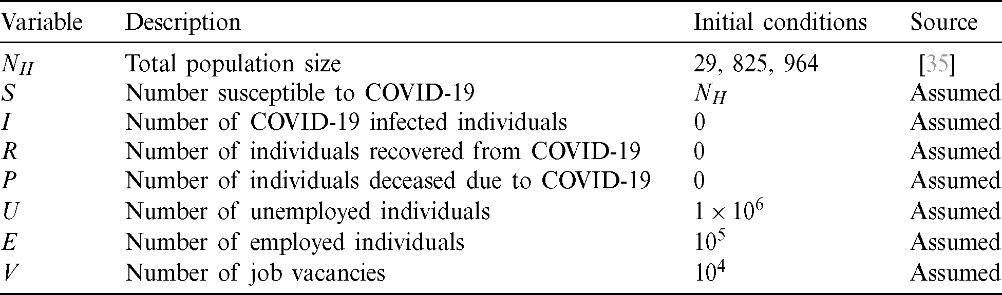
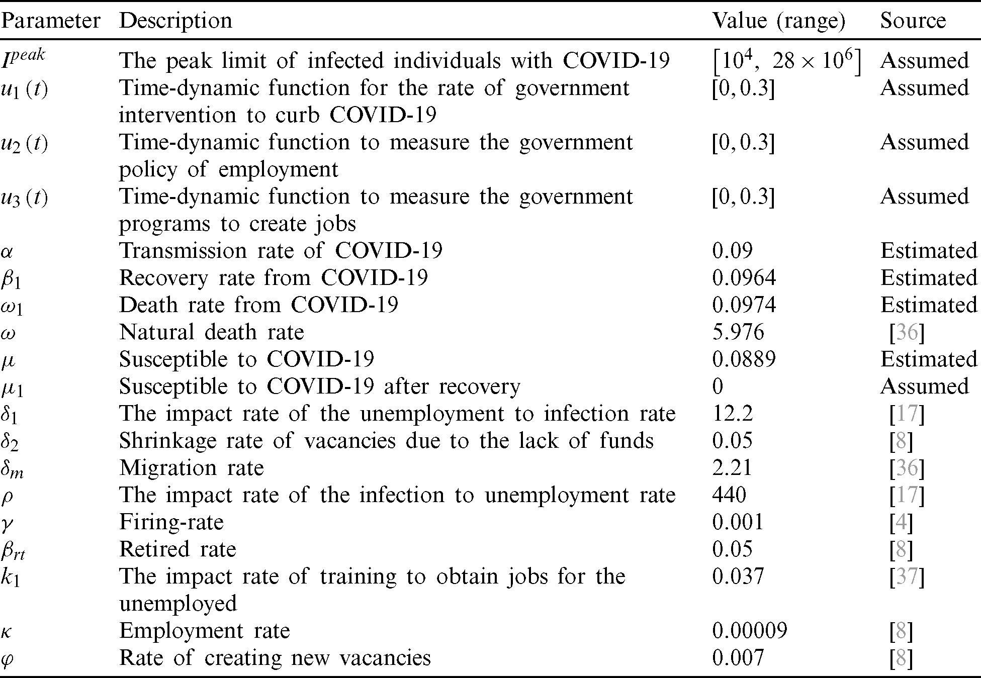
Table 2: Parameter definitions and value range
The classification of the population based on COVID-19 infection is:  and
and  corresponding to the individuals in the four epidemiological classes at time t. The total population at time t, denoted by N(t), is:

Moreover, the classification of population based on employment is  and
and  where the total population at time t is:

The following dynamic differential equation system defines both the COVID-19 and the employment model:


Eq. (3) defines all populations susceptible to COVID-19 infection. We assume that a fraction  of the population and a fraction
  of recovered individuals from COVID-19 infections are susceptible to COVID-19 infection. Leaving this class is carried out by infections with COVID-19 at a transmission rate of
  . An intervention suggested to minimize the number of infected with COVID-19
  is a time-variant variable that measures government interventions, for e.g., lockdowns and social distancing to curb the COVID-19 outbreak. Eq. (4) describes the COVID-19 infected individuals which comes from the susceptible class at rate
  The inputs to this epidemiological class can be controlled via government policy. This class will either recover at a rate of
  or succumb to death at rate
  . The parameter
  measures the effect of unemployment on the infected class. Eq. (5) describes individuals recovered from COVID-19. This class is increased by the recovery of affected individuals at rate
  . Moreover, this class is decreased by re-infection with COVID-19 at rate
  . Eq. (6) describes the individuals who succumbed to COVID-19 at rate
  . The remaining three equations describe the unemployment model. Eq. (7) defines unemployed individuals. The inflow is due to those seeking work but unable to find it because of the COVID-19 infection; layoffs; or the negative repercussions on the economy. Reducing the inflow occurs by finding jobs, emigration, natural death, death due to COVID-19, or by retirin. The government aims to reduce the number of unemployed by honing their skills and training them to become qualified and skilled for vacant jobs (expressed by the time-variant variable
  ), or by creating new job opportunities and expressed by the time-variant variable
  . Eq. (8) expresses the class of employees. This class increases when the unemployed find jobs and decreases via emigration, retirement, natural death, death due to COVID-19, or when being fired or laid off from either the pandemic or economic stagnation. Eq. (9) defines vacancies, which is increased either by creating new jobs or training the unemployed with high skills that are able to fill vacant jobs or employees leaving their job for any reason so that their jobs become vacant. Meanwhile, the number of vacancies decreases due to economic stagnation, disasters, or the COVID-19 pandemic.
3 Bi-Level Dynamic Optimal Control Problem
Bi-level optimization is NP-hard because of its hierarchical structure, which combines more than one model so that one is nested within the other. The outer model is called the leader or the upper-level, and the inner model is the follower or the lower-level. Thus, bi-level optimization can be formulated as:
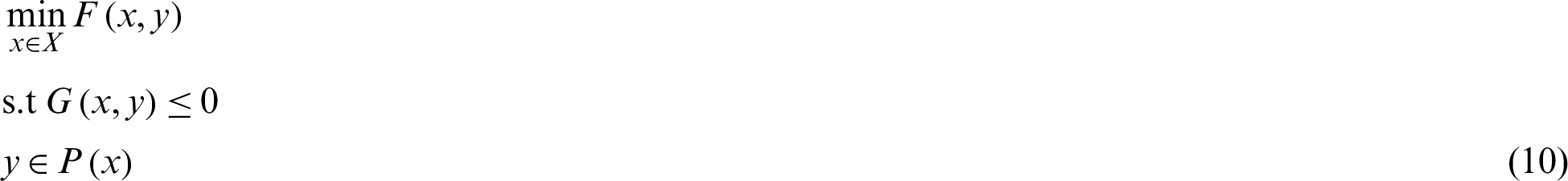
where
where  is the upper-level objective with respect to the decision variable x and the constraints
  . The constraints of the upper-level problem include the optimal solution to the lower-level objective
  with respect to the decision variable y and the constraints
  .
.
In our paper, the bi-level dynamic optimal control model (BLDOC) contains the COVID-19 model as the leader and the unemployment model as the follower. The BLDOC formulation is defined through the following equations:
MODEL I:
Upper Level


Lower Level


Eq. (11) represents the objective function of the upper level and Eq. (20) that of the lower level, which minimize the infected individuals with COVID-19 and the number of unemployed respectively; and minimizes the cost associated with the interventions of control. Eq. (10) defines the maximum infected individuals with COVID-19. Eqs. (12)–(15), (21) and (22) determine the bounds of the time-varying variables which can be changed to determine the best control strategy. Eqs. (16)–(19) represent COVID-19 dynamic constraints, while Eqs. (22)–(25) represent unemployment dynamic constraints. And z1, z2, A, B, and C are weight coefficients. The optimal control model is assumed during the full-time horizon  , where tf is 52 weeks.
4 The BLDOC Model Solution Approach
This section presents our model solution methodology. First, we will find the Lagrangian function of the lower-level model to be used to reformulate the proposed model. Second, the lower level problem is replaced by a modified approximation of the KKT condition. Third, we will derive the Hamiltonian function from the Lagrangian function to be used to reformulate the proposed model.
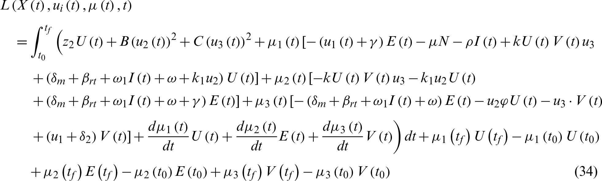
The Lagrangian function of the lower-level model is:
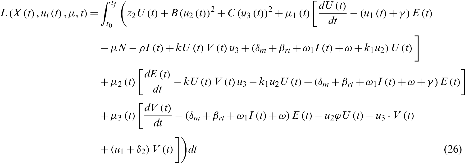
where  , and
, and  are time functions compared to the Lagrange multipliers in a static optimization model.
  refers to the unemployment classes
  ,
,  , and
, and  .
.
In the bi-level optimization, although the KKT conditions of the lower–level can often be used to convert the model to a single-level model, the KKT conditions cannot be used for all models, especially the BLDOC, due to the KKT’s non-convexities. Thus, we will use the modified approximation KKT condition.
The formulation of the single-level obtained by substituting the lower-level with the modified approximation KKT conditions is:
MODEL II


where  is a small number bounded by the fixed-parameter
  .
.
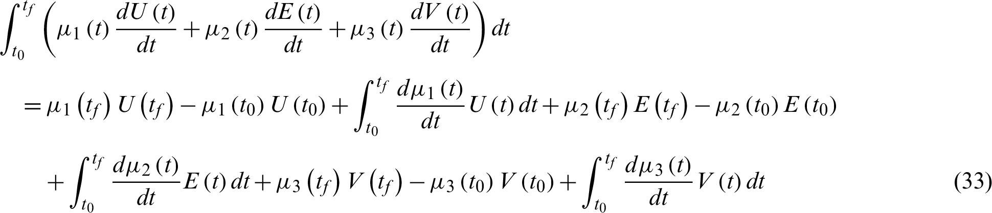
Now, the Hamiltonian function can be derived from the Lagrangian function. In Eq. (26), partial integration can rewrite the last term on the right-hand side as:
Substitute Eq. (33) into the Lagrangian function Eq. (26) to obtain:
The total derivative of Lagrangian function obeys:
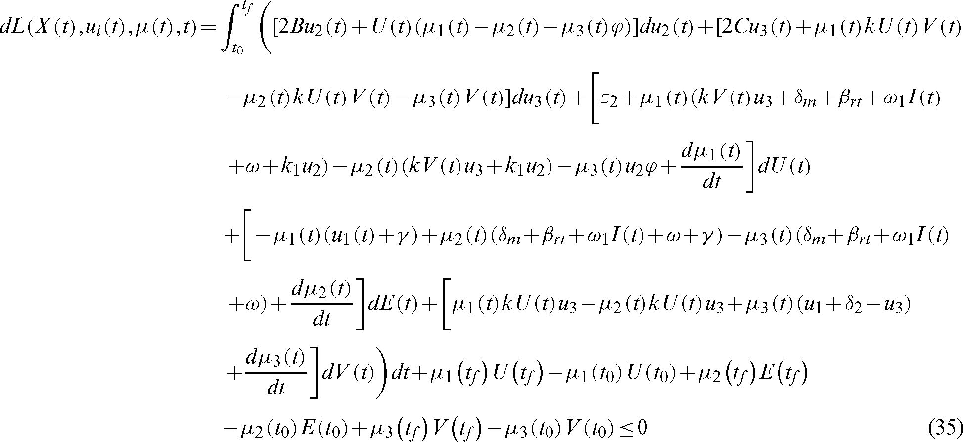
:
The  and
and  are fixed; thus, their derivates equal zero. We obtain the following equations, which are equivalent to Eq. (28)


MODEL II can then be rewritten as:
MODEL III:


In this section, we set the initial conditions of each class as reported in Tabs. 1 and 2. We assume the weights z1, z2, A, B, and C equal 1 for all simulations. The range of the active control variables are 
 0.3 and the values of the inactive control variables are equal to zero. The algorithm was implemented in Python 3.7.
The population change was obtained for each class with and without government interventions (See Fig. 1). For non-intervention, we can see from Fig. 1, Panel (B) that the curves of active infected, perished, and recovered persons increase steadily without stability over the sample period.
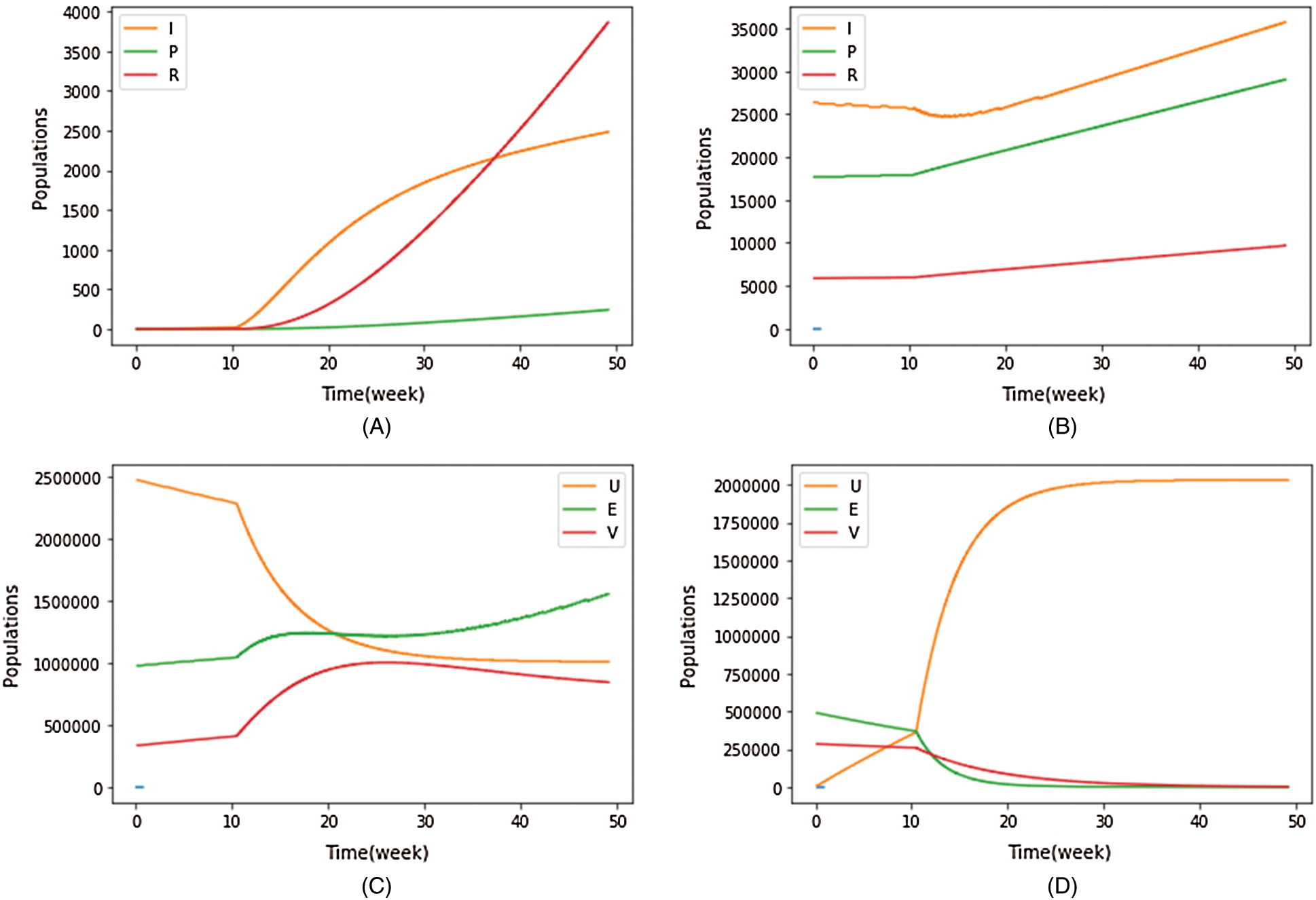
Figure 1: Population classes trajectories for with/without control cases
In the case of the interventions (see Panel (A)), the number of active infected, and thus the deceased and recovered individuals are few compared to the uncontrolled case; and we can see that the curve of the infected individuals stabilizes with a slow increase without declining during the sample period.
Similarly, from Fig. 1, Panels (C) and (D) illustrate the importance of government intervention in controlling the number of unemployed and the vacancies.
In the absence of intervention (see Panel (D)), the number of unemployed increases dramatically, while the number of employees and vacancies decrease.
Pertaining to government interventions (Panel (C)), the number of employees and the number of vacancies increases, which then decreases the number of unemployed.
Three control variables are now used for the simulation. We present the following four cases which investigate all or some the control variables:
Case 1:  ,
,  and
and  0
0
Here, we assume the three control variables are active at both levels. The government has implemented measures to curb COVID-19 through quarantining infected individuals, social distancing, and providing personal protection. In addition, the government has implemented policies for developing labor market skills and for creating new jobs.
Case 2: u1 = 0, u2 = 0, and u3 = 0
Here, we assume the three control variables to be inactive at both levels, where the government has neither implemented measures to curb COVID-19, nor introduced policies to reduce the unemployment rate.
Case 3: u1 = 0,  and
and  0
0
Here, the government has intervened only to reduce unemployment, without taking any measures to curb COVID-19. Government unemployment policies include: refining the skills of the unemployed to enable them to find jobs; creating new jobs, whether directly or by revitalizing the economy and tourism; and reducing taxes.
Case 4:  , u2 = 0, and u3 = 0
Here, the government’s objective is only to curb COVID-19, while not reducing the unemployment rate. Measures include full lockdown, which of course directly affects the economy and the unemployment rate as well.
Fig. 2 compares the four cases. Panel A, which illustrates the number of active infected with the COVID-19 epidemic in all four cases, shows significant differences in the absence of the control case and the others. The number of active infected individuals may reach 50,000 cases without the control (Case 2) while in the other cases it does not exceed 10,000 cases.
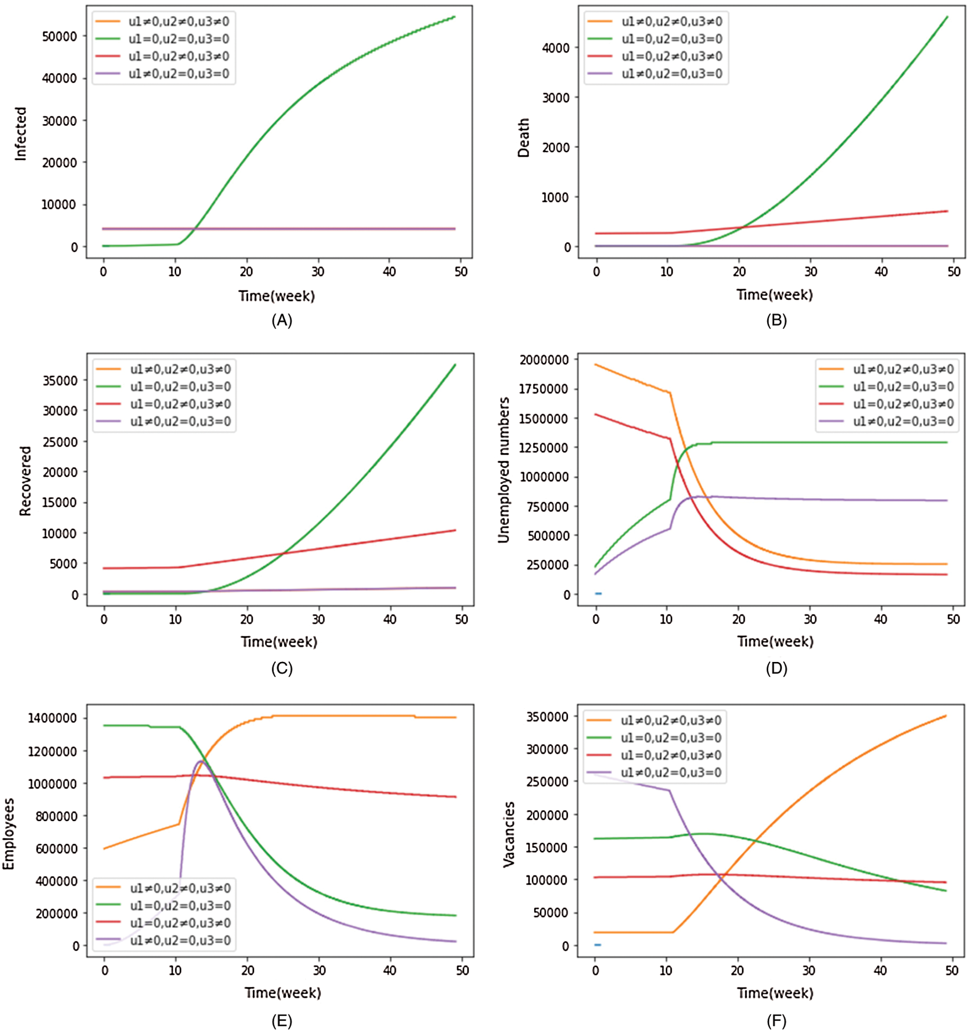
Figure 2: Comparing the simulation results of the control variables for all the four cases
From Panel (B) in Fig. 2, the deceased due to COVID-19 are relatively large in the absence of intervention and may reach two thousand individuals, followed by Case 3. The numbers of the deceased perished in Case 1 and Case 4 are the lowest.
Panel (C) indicating those who recovered from COVID-19 shows that the number of recovered individuals is large in the absence of the control case, the result of a large number of infected individuals, followed second by Case 4. In the other two cases, the number of recovered individuals is relatively small, due to the small number of infected individuals.
Panel (D) indicates that the number of unemployed increased dramatically with no measures to curb COVID-19 or reduce unemployment. It increases slowly in Case (4) when the government took measures only to confront COVID-19 without taking any measures to reduce unemployment. The number of unemployed decreases when the government intervenes to reduce unemployment, with or without measures to curb COVID-19, as is in Cases (1) and (3).
Panel (E) illustrates the dynamic changes in employees for all strategies. It is clear that the number of employees decreases in Cases (2) and (4), whereas the number of employees increases when the government takes measures to reduce unemployment.
Likewise, vacancies increase when the government takes measures to create new jobs. See Panel (F) in Case 1, wherein it is almost stable in Case 3 while the number of vacancies shrinks in Cases (2) and (4), when the government does not intervene to reduce unemployment.
The costs associated with applying Case (3) is the highest, followed by Case (1), whereas Case (2) has the lowest expenditure involved.
Thus, we need to balance between measures to curb COVID-19 and interventions to reduce unemployment. The measures cannot be taken to solve any problem without studying its effects on the other nested problems. Therefore, holistic studies are necessary to determine the community’s priorities, and the necessary weights for each problem. Based on our results, measures to fight both COVID-19 and unemployment (i.e., Case (1)) is the optimal strategy, with the possibility of changing the intervention weights based on society’s preferences.
In this paper we used bi-level programming to investigate the interaction between the COVID-19 pandemic and unemployment. We used the COVID-19 model as a leader and the unemployment model as a follower. The objectives of this model are to minimize the number of infected individuals with COVID-19 and the number of unemployed and to minimize the costs associated with different controls. The modified approximation KKT with the Hamiltonian function was utilized to convert the bi-level model into a single-level model. Three control variables were considered: The first control variable relates to government measures to curb the COVID-19 pandemic, i.e., quarantine, social distancing, and personal protection; and the other two control variables relate to government interventions to reduce the unemployment rate, whether through employment, making individuals qualified, creating new jobs, reviving the economy, reducing taxes, and other factors that may help reduce the unemployment rate. Four different cases were investigated to verify the effect of control variables, and the results showed the importance of balance between government measures to fight COVID-19 and government interventions to preserve the economy and reduce the unemployment rate. As a future suggestion, the introduction of a robust optimization model can be considered.
Funding Statement: The authors extend their appreciation to the Deanship of Scientific Research at King Saud University for funding this work through research Group No. RG-1441-309.
Conflicts of Interest: The authors declare that they have no conflicts of interest to report regarding the present study.
References
1. A. Bauer and E. Weber, “COVID-19: How much unemployment was caused by the shutdown in Germany?,” Applied Economics Letters, vol. 11, pp. 1–6, 2020.
2. P. Stroud, “Poverty and COVID-19: A report of the social metrics commission,” Legatum Institute, pp. 1–23, 2020.
3. A. Sumner, C. Hoy and E. Ortiz–Juarez, “Estimates of the impact of COVID-19 on global poverty,” In: UNU–WIDER, Helsinki, Finland, 2020.
4. S. B. Munoli and S. Gani, “Optimal control analysis of a mathematical model for unemployment,” Optimal Control Applications and Methods, vol. 37, no. 4, pp. 798–806, 2016.
5. S. B. Munoli, S. R. Gani and S. R. Gani, “A mathematical approach to employment policies: An optimal control analysis,” International Journal of Statistics and Systems, vol. 12, no. 3, pp. 549–565, 2017.
6. A. B. Kazeem, S. A. Alimi and M. O. Ibrahim, “Threshold parameter for the control of unemployment in the society: Mathematical model and analysis,” Journal of Applied Mathematics and Physics, vol. 6, no. 12, pp. 2563, 2018.
7. R. M. Al-Maalwi, H. A. Ashi and S. Al-sheikh, “Unemployment model,” Applied Mathematical Sciences, vol. 12, no. 21, pp. 989–1006, 2018.
8. A. Galindro and D. F. M. Torres, “A simple mathematical model for unemployment: A case study in Portugal with optimal controly,” Statistics Optimization & Information Computing, vol. 6, no. 1, pp. 116–129, 2018.
9. L. Harding and M. Neamţu, “A dynamic model of unemployment with migration and delayed policy intervention,” Computational Economics, vol. 51, no. 3, pp. 427–462, 2018.
10. A. K. Misra, A. K. Singh and P. K. Singh, “Modeling the role of skill development to control unemployment,” Differential Equations and Dynamical Systems, vol. 21, no. 12, pp. 1–3, 2020.
11. T. Kuniya, “Prediction of the epidemic peak of coronavirus disease in Japan,” Journal of Clinical Medicine, vol. 9, no. 3, pp. 789, 2020.
12. A. Kucharski, T. Russell, C. Diamond, S. Funk, R. Eggo et al., “Early dynamics of transmission and control of 2019-nCoV: A mathematical modelling study,” Lancet Infectious Diseases, vol. 20, no. 5, pp. 553–558, 2020.
13. M. Mandal, S. Jana, S. K. Nandi, A. Khatua, S. Adak et al., “A model based study on the dynamics of COVID-19: Prediction and control,” Chaos Solitons and Fractals, vol. 136, 109889, 2020.
14. S. Lalmuanawma, J. Hussain and L. Chhakchhuak, “Applications of machine learning and artificial intelligence for COVID-19 (SARS-CoV-2) pandemic: A review,” Chaos Solitons and Fractals, vol. 139, 110059, 2020.
15. F. Ndaïrou, I. Area, J. J. Nieto and D. F. M. Torres, “Mathematical modeling of COVID-19 transmission dynamics with a case study of Wuhan,” Chaos Solitons and Fractals, vol. 135, 109846, 2020.
16. A. R. Tuite, D. N. Fisman and A. L. Greer, “Mathematical modelling of COVID-19 transmission and mitigation strategies in the population of Ontario, Canada,” Canadian Medical Association Journal, vol. 192, no. 19, pp. E497–E505, 2020.
17. M. Cristina and B. Goes, “A Predator–prey model of unemployment and w-shaped recession in the COVID-19 pandemic,” New School for Social Research Department of Economics, 2006, pp. 1–12, 2020.
18. A. Sinha, P. Malo and K. Deb, “A Review on bilevel optimization: From classical to evolutionary approaches and applications,” IEEE Transactions on Evolutionary Computation, vol. 22, no. 2, pp. 276–295, 2018.
19. K. Palagachev, “Mixed-integer optimal control and bilevel optimization: Vanishing constraints and scheduling tasks,” Ph.D. dissertation, Bundeswehr University Munich, Germany, 2017.
20. J. J. Ye, “Necessary conditions for bilevel dynamic optimization problems,” SIAM Journal on Control and Optimization, vol. 33, no. 4, pp. 1208–1223, 1995.
21. K. D. Palagachev and M. Gerdts, “Numerical approaches towards bilevel optimal control problems with scheduling tasks,” in L. Ghezzi, D. Hömberg and C. Landry, Math for the Digital Factory, vol. 27, Cham: Springer, pp. 205–228, 2017.
22. F. Benita and P. Mehlitz, “Bilevel optimal control with final-state-dependent finite-dimensional lower level,” SIAM Journal on Optimization, vol. 26, no. 1, pp. 718–752, 2016.
23. F. Benita, S. Dempe and P. Mehlitz, “Bilevel optimal control problems with pure state constraints and finite-dimensional lower level,” SIAM Journal on Optimization, vol. 26, no. 1, pp. 564–588, 2016.
24. K. Palagachev and M. Gerdts, “Exploitation of the value function in a bilevel optimal control problem,” in IFIP Advances in Information and Communication Technology, France: Sophia Antipolis, pp. 410–419, 2015.
25. C. Christof, “Gradient-based solution algorithms for a class of bilevel optimization and optimal control problems with a non-smooth lower level,” SIAM Journal on Optimization, vol. 30, no. 1, pp. 290–318, 2020.
26. M. Knauer, “Fast and save container cranes as bilevel optimal control problems,” Mathematical and Computer Modelling of Dynamical Systems, vol. 18, no. 4, pp. 465–486, 2012.
27. V. Suryan, A. Sinha, P. Malo and K. Deb, “Handling inverse optimal control problems using evolutionary bilevel optimization”, in IEEE Cong. on Evolutionary Computation, Vancouver, Canada: IEEE, pp. 1893–1900, 2016.
28. Y. Wang, H. Li and C. Dang, “A new evolutionary algorithm for a class of nonlinear bilevel programming problems and its global convergence,” INFORMS Journal on Computing, vol. 23, no. 4, pp. 618–629, 2011.
29. A. Sinha, P. Malo and K. Deb, “Evolutionary algorithm for bilevel optimization using approximations of the lower level optimal solution mapping,” European Journal of Operational Research, vol. 257, no. 2, pp. 395–411, 2017.
30. A. Sinha, P. Malo and K. Deb, “An improved bilevel evolutionary algorithm based on quadratic approximations,ȝ in Proc. of the 2014 IEEE Cong. on Evolutionary Computation, Beijing: IEEE, pp. 1870–1877, 2014.
31. S. Shi, Y. Xiong, J. Chen and C. Xiong, “A bilevel optimal motion planning model with application to autonomous parking,” International Journal of Intelligent Robotics and Applications, vol. 3, no. 4, pp. 370–382, 2019.
32. S. Albrecht and M. Ulbrich, “Mathematical programs with complementarity constraints in the context of inverse optimal control for locomotion,” Optimization Methods and Software, vol. 32, no. 4, pp. 670–698, 2017.
33. A. A. Kahloul and A. Sakly, “Hybrid approach for constrained optimal control of nonlinear switched systems,” Journal of Control, Automation and Electrical Systems, vol. 31, no. 4, pp. 865–873, 2020.
34. A. Sinha, T. Soun and K. Deb, “Using Karush–Kuhn–Tucker proximity measure for solving bilevel optimization problems,” Swarm and Evolutionary Computation, vol. 44, pp. 496–510, 2019.
35. Worldometers, “Yemen population,” 2020. [Online]. Available: https://www.worldometers.info/worldpopulation/yemen-population/.
36. Macrotrends, “Macrotrends,” 2020. [Online]. Available: https://www.macrotrends.net/1316/us-nationalunemployment-rate?q=yemen.
37. U. K. Mallick and M. H. A. Biswas, “Mathematical approach with optimal control: Reduction of unemployment problem in Bangladesh,” Journal of Applied Nonlinear Dynamics, vol. 9, no. 2, pp. 231–246, 2020.
 | This work is licensed under a Creative Commons Attribution 4.0 International License,, which permits unrestricted use, distribution, and reproduction in any medium, provided the original work is properly cited. |