DOI:10.32604/cmc.2021.014599
| Computers, Materials & Continua DOI:10.32604/cmc.2021.014599 | |
| Article |
Epithelial Layer Estimation Using Curvatures and Textural Features for Dysplastic Tissue Detection
1Faculty of Information Science and Technology, Center for Artificial Intelligence Technology, Universiti Kebangsaan Malaysia, Bangi, Selangor, 43300, Malaysia
2Faculty of Science and Technology, School of Mathematical Sciences, Universiti Kebangsaan Malaysia, Bangi, Selangor, 43300, Malaysia
3Department of Information Technology and Computing, Faculty of Computer Studies, Arab Open University, Amman, Jordan
*Corresponding Author: Afzan Adam. Email: afzan@ukm.edu.my
Received: 02 October 2020; Accepted: 14 November 2020
Abstract: Boundary effect in digital pathology is a phenomenon where the tissue shapes of biopsy samples get distorted during the sampling process. The morphological pattern of an epithelial layer is greatly affected. Theoretically, the shape deformation model can normalise the distortions, but it needs a 2D image. Curvatures theory, on the other hand, is not yet tested on digital pathology images. Therefore, this work proposed a curvature detection to reduce the boundary effects and estimates the epithelial layer. The boundary effect on the tissue surfaces is normalised using the frequency of a curve deviates from being a straight line. The epithelial layer’s depth is estimated from the tissue edges and the connected nucleolus only. Then, the textural and spatial features along the estimated layer are used for dysplastic tissue detection. The proposed method achieved better performance compared to the whole tissue regions in terms of detecting dysplastic tissue. The result shows a leap of kappa points from fair to a substantial agreement with the expert’s ground truth classification. The improved results demonstrate that curvatures have been effective in reducing the boundary effects on the epithelial layer of tissue. Thus, quantifying and classifying the morphological patterns for dysplasia can be automated. The textural and spatial features on the detected epithelial layer can capture the changes in tissue.
Keywords: Digital pathology; grading dysplasia; tissue boundary effect
Digital and computational pathology are becoming in demand now for clinical diagnosis and education, and a recent study in oral pathology [1] is the latest proof. The demand is motivated by the current inter and intra-observer variations, fuzzy areas of grading, and the repetitive and time-consuming process of diagnosing pathology slides.
Tissue changes, known as morphological transitions, are continuous and vary over time, rendering diagnosis more difficult at higher stages due to their complexity [2]. However, detecting and grading dysplasia are routine in histopathological diagnosis as they determine the first signs of tissue changes. Therefore, Shaheen et al. [3] have identified the guidelines for the patients with non-dysplastic Barrett’s Oesophagus (BO) and their endoscopic surveillance.
Dysplasia, in BO, is characterised by morphological transitions in oesophagus lining where mucus-secreting goblet cells and glands start to form in the epithelium and lamina propria. Then, the condition may progress into low-grade dysplasia where size, shape, and other cytological features in the cells and nuclei, starts to morph. The micro changes will gradually be seen in oesophagus lining, as the smooth surface of the squamous epithelial layer begins to form a fingerlike cellular pattern, also known as villiform. The pattern becomes more complicated with back-to-back gland formations and more prominent nuclei sizes, and other abnormalities invade into lamina or even the muscularis mucosa area, a sign of invasive carcinoma. Fig. 1 are sample tissue in varying dysplasia grade to show the changes in patterns.
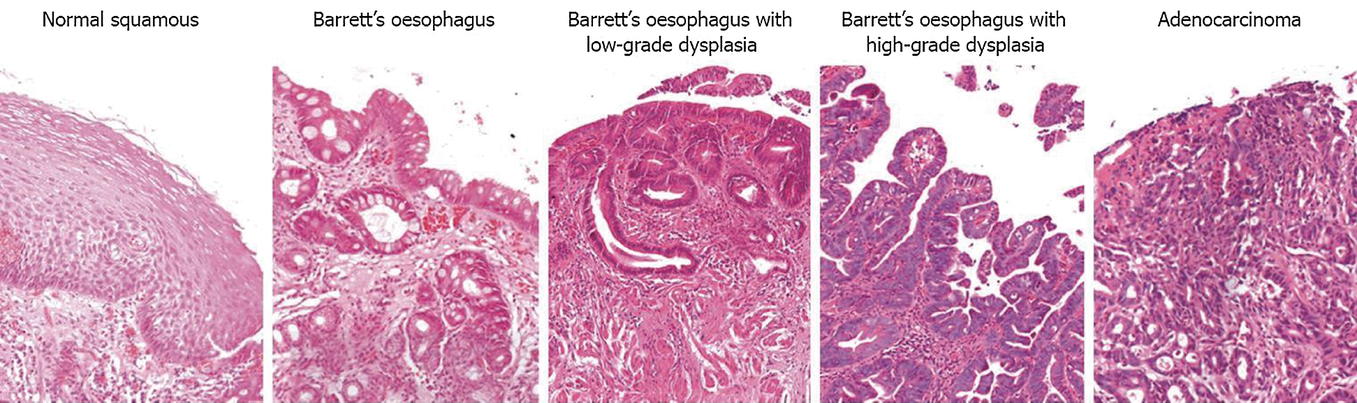
Figure 1: Transition from normal squamous epithelial cells into intestinal metaplasia [4]
A trained pathologist can usually detect tissue changes under a light microscope, but the inter-observer agreement for dysplasia is generally less than moderate. On top of this, sampling error at the time of endoscopy may contribute to the diagnosis of BO [5,6]. Different pathologists have their own interpretations and opinions of the histopathological definitions of dysplastic epithelial lesions. Based on years of experience with dysplastic tissue, an agreement is not always met [7,8]. Although the conclusions mentioned above were reached 16 and 12 years back respectively, the recent research on dysplasia grading agreements in 2014 and 2016 show that the findings are still valid as the agreement on colon and oral epithelial indefinite dysplasia score less than 0.3 kappa (fair agreement) [9,10]. Meanwhile, the most recent report on BO tissue verified that the variations in agreement among experts concerning dysplasia across all grades had been 0.58 since ten years ago [11]. Besides, an online consensus of 50 pathologists from over 20 countries reveals histopathologist-dependent predictors of significant diagnostic error in the assessment of Barrett’s biopsies [12], and grading dysplasia accurately is still reported as a challenging task [13]. Kaye et al. [14] has also concluded that preventing the over-diagnosing of dysplasia may avoid inappropriate treatment.
Thus, implementing machine learning to help identify and measure morphological transition patterns may help in reducing the variations. Recent attempts on implementing machine learning on histopathology images are on the oesophagus, using textural and spatial features [15]. There is also research applying machine learning on blood peripheral film image using shapes features [16], and brain using shapes and spatial features [17]. Besides, grading prostate and breast cancer [18–20], endoscopy [21], oncology [22], liver disorder [23] and colon [24], were also attempted, among others.
Oesophagus tissue usually is of a smooth line shape, but during sampling, they are pinched off or scraped from the oesophagus lining. The process yields curvature-shaped tissue for the biopsy, known as ‘boundary effect’. Tissue samples located in the surface area are usually affected, such as the epithelial layer in the mouth, oesophagus, colon and cervical biopsies. In characterising dysplasia, examining the epithelium layer is essential [25,26]. As shown in Fig. 1, normal tissue, low-grade dysplasia and adenocarcinoma shared the same tissue surface characteristics, which is smooth. The inner texture gives away the differences while Barrett’s oesophagus and the high-grade dysplasia usually have curvy surfaces. Therefore, the effect from pinching off the tissue while sampling may introduce unnecessary curves along the tissue surfaces. Manual detection and characterisation of dysplastic regions in pathology images are labour-intensive and subjective. Therefore, we proposed an automated region detection and boundary effects must be taken into consideration for handling false positives regions.
Meanwhile, in the machine vision field, it is agreed that the shapes and curvatures of biopsy sample tissues have a significant impact on tissue architecture analysis [11,27–30]. Recent works involving tissue shaped and boundary-related challenges include segmentation of deep brain regions [31], learning shape and appearance models to improve deformation smoothness [32] as well as using a deformable model to estimate the correct shape [11,33]. Curvatures theory in measuring surface deviation degree from being a plane on tissue images is not yet found in any literature.
The main objective of this paper is to identify dysplastic tissue from the epithelial layer. However, the epithelial layer is greatly affected by boundary effects during the biopsy sampling processes. Thus, one of the significant contributions of this paper is the curvature-based method for detecting and extracting the correct epithelial tissue texture from the digital slide. This is because curvature theory on tissue boundary or squamous epithelial layer is not yet found in any literature. The proposed method has enabled the analysis of textural feature along the curvy tissue surface and solved the boundary effect problem.
Then, rigorous experiments to find the correct thickness of the epithelial layer in each particular zoom level for these regions were carried out. The second contribution is the new texture features called cluster co-occurrence matrix (CCM), which preserves and correlates the textural and spatial features between different magnifications. Considering spatial information between clusters of image texture has enabled the algorithm to capture different primitives on tissue images, without the need to identify them. The CCM feature extractions are carried out in two levels of magnification for each selected region and used in the machine learning approach for tissue classification.
This paper is organised as follows: Section 2 describes the methodology used including datasets and the processes for tissue detection, segmentation to region and type of tissues, as well as the feature extraction and classification from the curvy and smooth-surfaced virtual slides. Theories that underpins the shape complexity measurement also presented. The parameter and feature selection for epithelial layer classification is also explained. Then, Section 3 follows, describing the result obtained from experiments carried out to normalise the boundary effects of tissue shape and the estimation of epithelial thickness. It also includes the boundary complexity quantifiers after the normalisation of the boundary effect and the CCM feature performance in classifying dysplastic tissue. In Section 4, discussions on the findings from all experiments to show the significance and relationship of the machine learning and machine vision modelling to the domain understandings are carried out.
Tissue structure, as defined collectively by [4,11,29,34,35], is a general organisation or pattern of cellular geometric or reciprocal arrangements with other cellular structures within a tissue. Therefore, selecting correct regions from the whole virtual slides is very important, to detect the changes in tissue structure in different stages of dysplasia. Also, the virtual slides contained several unarranged tissues from more than one biopsy sample. The analysis was conducted in five stages, as illustrated in Fig. 2. It started with detecting tissues from the whole slides at five magnification level, where each level is a refinement from the previous ones. The at  magnification, curvature points will be detected and used at stage 2 to create regions. Regions created were magnified into
  magnification, and boundary lines detection is carried out with morphological operators and colour deconvolutions.
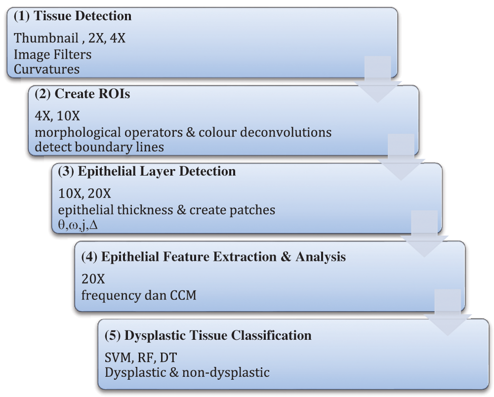
Figure 2: The processes involved in quantifying tissue boundary complexity and classifying dysplastic tissue
Stage 3 is to detect the epithelial layer in regions using the boundary lines detected at the previous stage. The layer thickness level is estimated with few parameters which will be elaborated in 2.4. The analysis of textural features will be carried out on the detected epithelial layer at  and the elaboration is in Section 2.5. In the final stage, these tissue regions will be classified into dysplastic or non-dysplastic as elaborated in Section 2.6.
The dataset used in this paper was obtained from an Aperio Server at St James’s Hospital, scanned with an Aperio Scanner at  zoom level [36]. Permission to access the dataset can be acquired at Leeds Virtual Pathology Project at http://www. virtual pathology.leeds.ac.uk/research. Four hundred seventy-four annotated images with annotations from ExpertB and ExpertE, recorded across 142 virtual slides, was used as our ground truth. To test the hypothesis, focused was on Grade 1 (Barrett’s only without dysplasia) and Grade 5 (Barrett’s with High-Grade dysplasia). A total of 147 annotated images out of the ground truth data were Grade 1 while 59 were Grade 5. Annotated regions with tissue boundaries were carefully selected for necessary tissue inclusions, leaving 40 balanced data between these two grades.
Two regions were identified based on the general characteristics of the tissue: the epithelial tissue and the lamina propria. The architectural and cytological features in each region differentiate the two types, and both had different patterns in the morphological sequences as well. As dysplastic changes occurred in the epithelial layer, segregating both tissue types was crucial. Therefore, additional measurements were taken in different magnification levels, as shown in Fig. 2, to detect and segment out the epithelial tissues. The tissue shape complexity guided regions creations, and classification is carried out using the textural features of the detected epithelial layer.
Based on the morphological pattern described above, the smoothness of the tissue’s boundaries can be used to gauge the tissue condition. While the changes in tissue progressed and invaded other areas, regions with smooth, curvy or complex surfaces needed to be segregated. In this work, feature extraction for epithelial tissue was applied in different magnification levels for each virtual slide in our training dataset. The first process was to detect the tissue from the virtual slides. At this stage, the whole virtual slide was viewed as thumbnail-sized images, with tissue labelled as a foreground using binary classification from grey-level thresholding. The image background is the white areas outside tissues including any object sizes of less than 200 pixels (usually smears or torn tissues). The background pixels were eliminated, leaving only tissues. Fig. 3 shows the detected tissues after these processes, from the original image (a), binary image (b), and detected tissues labelled (c).
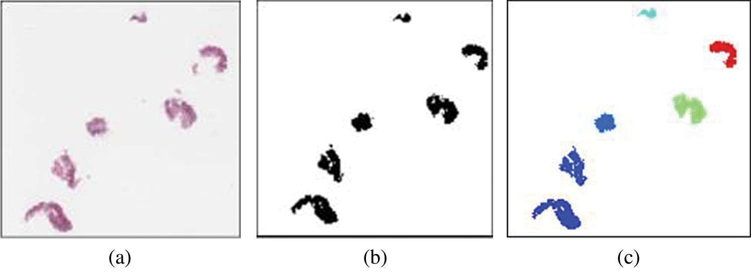
Figure 3: Tissue detected from whole slide images (thumbnail-sized). (a) Original image (b) binary image (c) labelled image
Knowing that normal oesophagus is covered with stratified squamous epithelium cells, different patterns of cells’ existence may show some abnormality. When dysplasia becomes more severe, the smooth lining eventually changes to form a villiform structure, similar to colon tissue. So, the detected tissues were further investigated in a binary format at  magnification, and each will be assigned with a bounding box. The coordinates of the intersection points between the candidate tissue and its bounding box, as well as all connected pixels with value ‘1’, excluding the bounding box itself, are recorded. These recorded coordinates represent the candidate tissue boundary (
 ). Then, the image with
  is used for shape analysis; so a good representation of the tissue shapes was needed. Few window sizes (j) along the
  were tested, as shown in Fig. 4 to select the best representation of the tissue shape. An appropriate j was important to ensure that the image representation is not too sensitive to small peaks and crypts, but still able to identify high curvature points along the
  . The pixels situated at the
  were considered as the boundary line
  , and the coordinates were recorded.
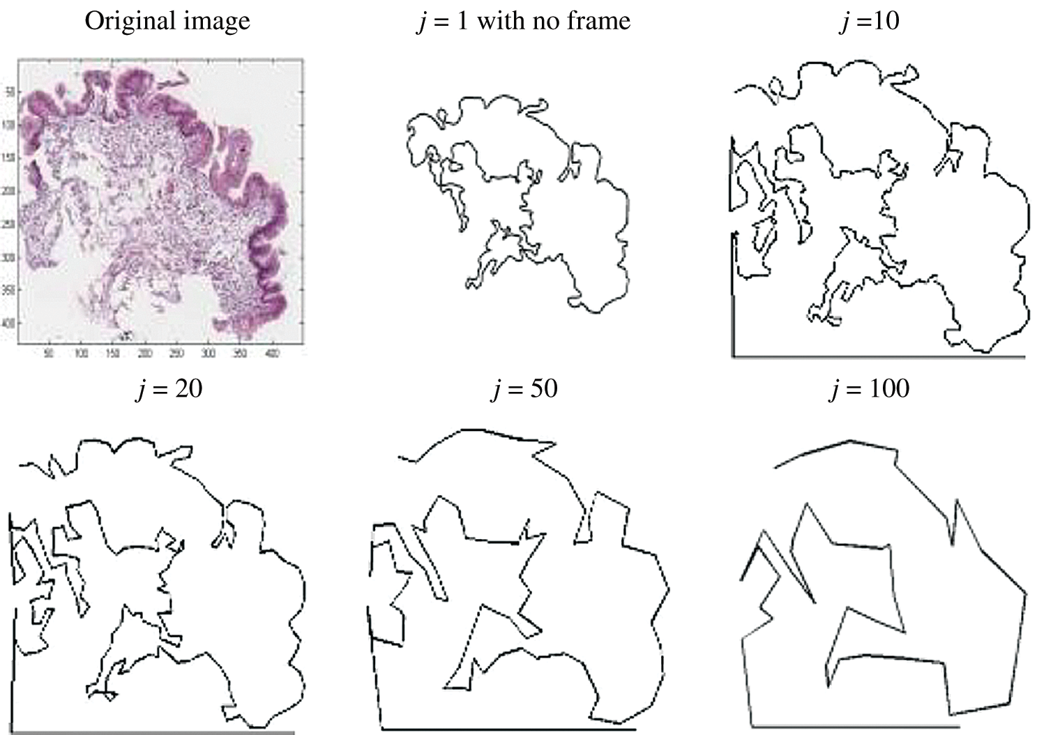
Figure 4: Image showing how different values of j affecting the tissue shape representation in  magnification
The high curvatures points (hc) (curvatures that fall between a specific range of angles [ 1,
1,  2]) identified along the
  is used to create the regions of interest. The hypotenuse of three consecutive j is used to calculated curvatures, as shown in Eq. (1). Then, the distances between hcs (
 ) and the standard deviation of distances (
 ) are calculated. Regions of interest (ROI) were created based on consecutive points that fell between the highest distances [
 ,
,  ]. This is to detect the smooth boundaries of normal squamous cells from the villiform patterns in the surface area. Each region repeats the same process at
  magnification, where detailed crypts and peaks in each ROI were measured. These ROIs were classified as complex or smooth boundaries using the frequency of hc along with a threshold distance of the
  .
.

where
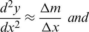
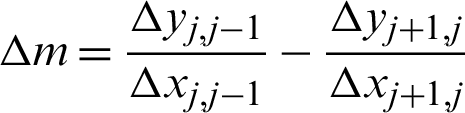
Fig. 5 below illustrates these processes. Referring to the illustration, (a), (a–d) are the points where the tissue boundary will be segmented. The first patch is from a to b, then from b to c, from c to d and lastly from d to a.
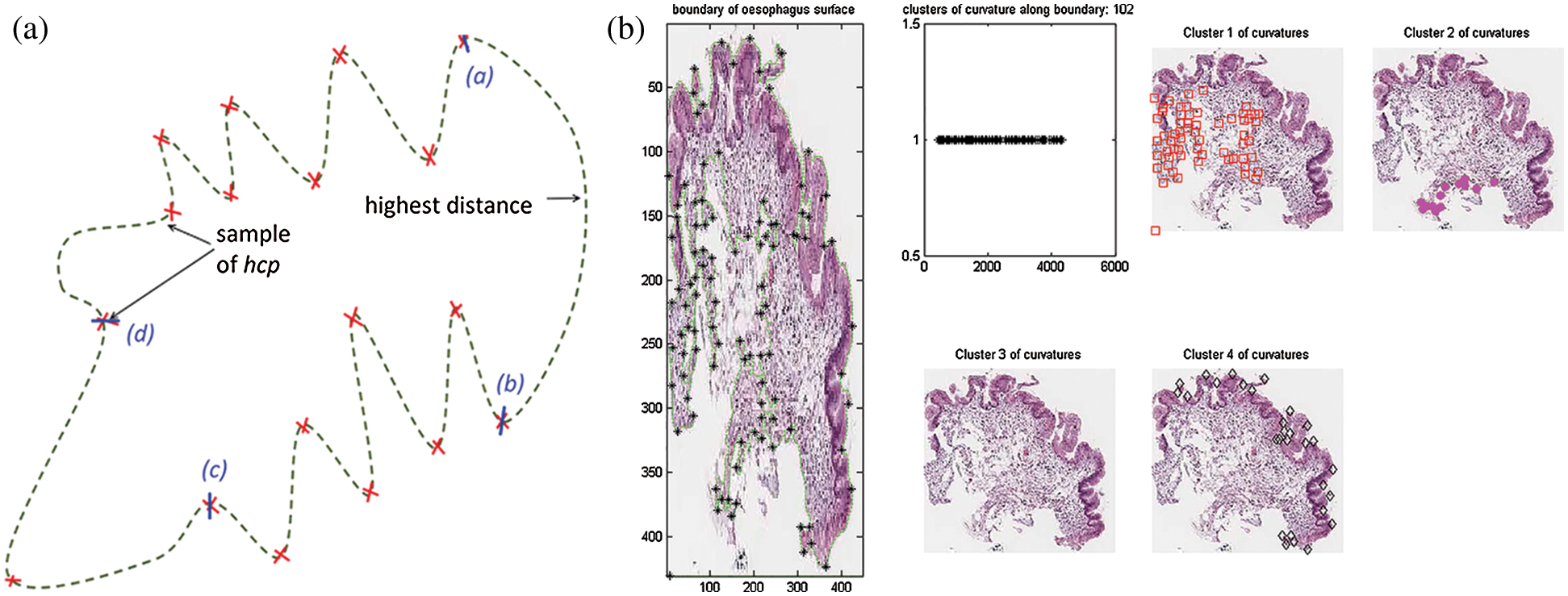
Figure 5: Region creation with curvatures. (a) Illustration of region creation on tissue boundary. (b) Implementation of region creation using curvatures on tissue boundary
2.4 Epithelial Layer Detection
Images of the ROIs created were accessed in  and
and  magnification levels to extract the epithelial tissue layer. At this zoom level, tissue appearance was more detailed; thus,
  needed to be detected again to enable a correct epithelial layer estimation. Therefore, two approaches were experimented to get the best tissue shape representation for
  detection at this magnification rates.
However, filters were applied to enhance the boundary detection accuracy and to retain unique coordinates. The coordinate of start-and-end points for each detected line are compared, and lines were linked together as one IF the coordinate is the same. The line measurements were recorded by the straight-line distance of the start-and-end points, and the number of connected pixels. The measurements were used as the third filter to verify the severity of surface complexity, as the detected line might be from torn tissue or the muscularis mucosa. Finally, the longest connected pixels detected was used as a priority for the candidate boundary. Fig. 6 shows the incorrectly detected boundary and the corrected version from these approaches.
Figure 6: Some of the wrongly-detected boundary and the corrected output for  c. Reasons for false detections: Image (a) missing starting pixel, image (b) longest detected line is not an epithelial tissue (c) longest line are the complex structure from torn-off tissue
The first method tested, was using optical density matrix for colour deconvolution in Hematoxylin and Eosin stained tissues, as suggested by Ruifrok et al., as the cytoplasm would appear pinkish and nuclei purplish. Applying this to an image produced a clearer image with enhanced nuclei or cytoplasm, making it easy to analyse each component further. The hypothesis was to extract the epithelial based on either nuclei lining or the cytoplasm in the ROI, as both components arranged themselves differently as dysplasia progressed. The nuclei component was deconvolved from each ROI. Then, repeated dilation and erosion processes were applied to the deconvolved ROI. This process was carried out to obtain the thinnest and smoothest line possible along the ROI boundary, without affecting the important crypts and peaks in the images. The line constructed was initialised as the candidate boundary:  n (from the deconvolved nuclei of ROI) and
  c (from the deconvolved cytoplasm of ROI).
The second approach is extracting the epithelial layer using the eight connected components. This method requires a binary image of ROI with the threshold grey-level values. From coordinate [0, 0], the coordinate for each connected pixel in eight directions, AND just next to a zero-valued pixel [background] was recorded as the boundary. Therefore, in each annotated region, a set of lines would be obtained, which would end at the bounding box but might start anywhere in the annotated regions. Five pixels on the image sides were excluded to ensure only relevant tissues are selected for boundary detection.
2.5 Epithelial Layer Tissue Texture Extraction
Next, the location and thickness of the epithelial tissue were detected using the two boundary coordinates [ n,
n,  c] detected before. For this, two coordinates perpendicular to both sides of the two
  s were calculated on every jth pixel. As illustrated in Fig. 7, point Aj is the jth pixels on the
  while point A
 and A″ are projected perpendicular to the line from Aj to Aj+1. The distances (R) of A
 and A″ from Aj represent the epithelial thickness. The grey-level values along the lines between points A and A
 , and from A to A″ on the original image were extracted. Higher grey-level values between the two sides were chosen as the epithelial area, as they contained lesser empty (background) pixels. Therefore, the coordinates for each accepted A
 or A″ were recorded, and the area between these lines and
  was considered as the epithelial tissue area.
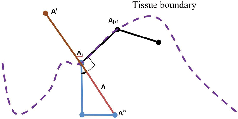
Figure 7: Illustration of patches projection from  to detect tissue areas and epithelial thickness
Annotated regions were analysed at  magnification for surface membrane feature extractions. As the tissue boundary was curvy, the squamous epithelial cells on the surface followed. Therefore, the effect of cell rotations at pixel-level need to be investigated. Thus, rotated and unrotated patches, as illustrated in Fig. 8 were considered. Patches along the
  were created using the moving coordinates of each jth pixel. This is carried out by calculating the slope between two neighbouring j, and the new coordinates for generating next patches were projected. Different patch heights [R = 100, 150, and 200 pixels] were selected to estimate the epithelial layer’s thickness for feature extraction. Ideally, patches should cover the whole epithelial layer only.
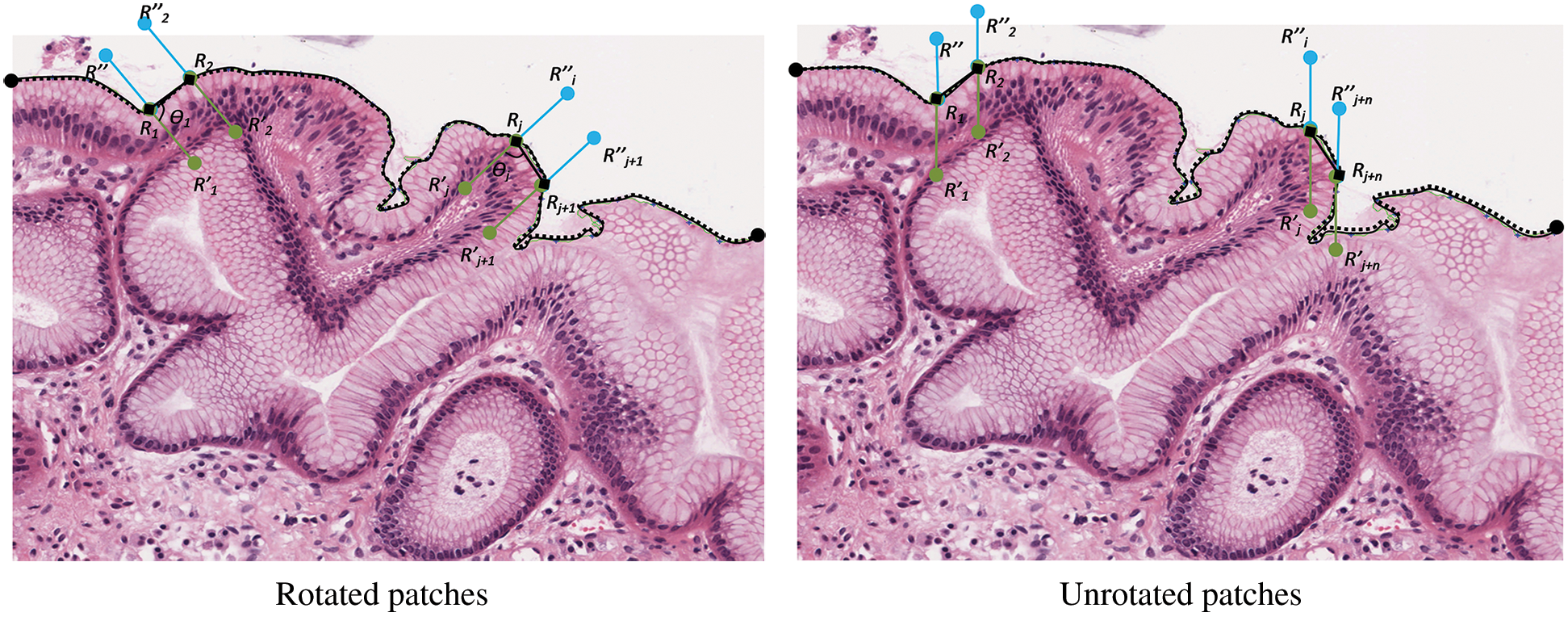
Figure 8: The creation of rotated and unrotated patches along the  c, at
c, at 
Next, the patches were transformed into greyscale images for feature extraction at the pixel level. GLCM features, namely contrast, correlation, energy, and homogeneity, were extracted in four directions from each patch to represent the patch texture. Then, K-means clustering will automatically cluster the patches based on their textural similarity into several clusters. Squared Euclidean Distance with two values of k was tested [k = 5, 7] for the evaluation process.
The GLCM features were used to investigate the effect of zoom-level and neighbouring distance [n] as well. Only this time, patches were created at  and
and  magnification levels with [n = 2, 4, 6, 8, 10]. The results presented in Tab. 4 show that the most reliable grading performance if from k = 5. The different numbers of n do not produce a significant difference in the accuracy percentage (AP), either at the same or different zoom level. In other inferences, when k = 7, the AP performances fluctuated across different values of n and zoom level.
Then, texture features at patch level were investigated. Three texture features from the rotated and unrotated patches along the epithelial layer from both  c and
c and  n were extracted and evaluated for comparison. The first texture was the cluster co-occurrence in one direction (
 ) along
  c and
c and  n, as described in [37]. The second was the frequency of clusters, and the third was the Local Binary Pattern (LBP) features. The LBP features were included to observe whether the CCM features on rotated and unrotated patches are directions invariant.
However, as the patches were aligned along the tissue boundary, the properties of the clusters in CCM (as in GLCM) were projected in one direction within two neighbouring patches. Therefore, eight features were extracted and used to differentiate between normal and dysplastic epithelial tissues in oesophagus virtual slides. The texture similarity between these patches was observed using ten-fold cross-validation on k-means clustering.
2.6 Dysplastic Tissue Classification
After feature extraction, the classifier model for classifying the annotated regions into dysplasia or non-dysplasia was trained. Decision Tree (DT), Random Forest (RF) and Support Vector Machine (SVM) classifier model were used on a 70% split-training test dataset to ensure the reliability and robustness of the results. The linear SVM was used, while the DT used was the C4.5 algorithm with a confidence factor of 0.25, and the minimum number of objects in each leaf was set as two. The RF built up to 100 trees with a maximum depth of 10.
Although deep learning is becoming a trend now in image classification and image detection, it lacks in explainable reasoning on how a decision is made [38–41]. Thus, domain understanding from the clinician for validation, clinical diagnosis and medicolegal issues will hinder its implementation in both education and diagnosis process.
This section presents the results of tissue boundary selection, region creation, boundary complexity identification, and the epithelial layer feature extraction and classification.
3.1 Curvature-Based for Boundary Complexity Quantifier
The first experiment was conducted to extract the correct  for region creation. Then, another 1628 brute-force experiments were carried out to establish an appropriate
  ,
,  1,
1,  2, and j. These variables are important to directly represent tissue boundary, shapes, and curvatures for segmenting correct regions.
Tab. 1 shows the parameters tested at  and
and  magnification levels and the best-selected value. At
  , j = 20 best at representing the peaks and crypts on the tissue boundary, while
  value ranging between
  and
and  was selected as a threshold of hc, with the
  as 200 pixels. At
  magnification, a boundary is classified as ‘complex’ when j was 40, and the
  value ranged between
  and
and  with at least 30 hc per 100 pixels as the
  value along with the epithelial layer. These values were established using 40 training patches annotated by a pathologist.
Table 1: Parameter setting for complexity measurement

Then, the  detection was carried out for each region classified as complex from previous steps. As explained in Section 3.2, the boundary detection results from nuclei and cytoplasm component [
 n and
n and  c] were both compared to hand-marked tissue boundary with Euclidean distance. Tab. 2 shows that the best result obtained was 82.5% AP from
  c, compared to only 47.5% using
  n. Thus,
  c was accepted as the tissue boundary for further processes. The experiment also showed that patches based on the
  c yielded better regions and lesser risked at crypts, but some information might be lost at a closed-curve boundary.
Table 2: Comparison of tissue boundary detection from different approaches

Then, feature extraction processes were carried out for the epithelial layer tissue, using  c as the baseline. Combinations of necessary parameter settings were tested to produce a good estimation of the epithelial layer thickness. Tab. 3 lists all the tested values for the parameters involved in the epithelial layer extractions and the selected best values.
Table 3: Parameters tested and selected values for epithelial layer detection

The effect of k, n, zoom were analysed with SVM. Tab. 4 shows that the best result is n = 4 at  magnification with five clusters.
Table 4: Validation result on values of n, k, and zoom level to classify annotated regions using the texture of the epithelial layer

In this step, the window sizes for patch creation were projected based on the  c. However, extra features such as the epithelial layer thickness were required, and the thickness varied, mostly when nuclei were at narrow crypts. From the experiments, R = 100 pixels are best in
  magnification.
Tab. 5 shows the comparison results for all classifiers, and the numbers are translated into Fig. 9 for better visualisation. The results indicated that the CCM features of the rotated and unrotated patches along the  c yielded better classification results than the frequency of clusters as well as the LBP. The features are generic enough that all three machine learning techniques give similar performance. Therefore, the CCM features extracted were also direction invariant. On the other hand, features from the frequency of clusters are more fluctuates with unrotated patches gives a lower performance, along with LBP features.
Table 5: Average classification result with ten-fold cross-validation for comparison of rotated and unrotated patches.

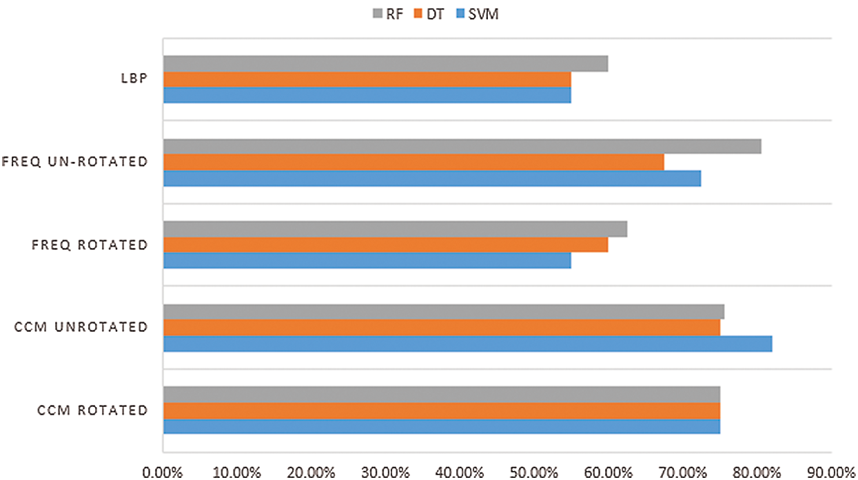
Figure 9: Comparison of classification accuracy between features
Tab. 6 shows the confusion matrix for dysplasia classification. The classification accuracy was 0.825 with 0.818 precision. The specificity was 0.789 while sensitivity was only 0.545 yield to 0.837 f score, which is considered good.
Table 6: Confusion matrix for epithelial layer dysplasia classification.

The selection of  shows that
  n was too sensitive to the nuclei size and location changes. Thus, many small crypts and peaks were detected, which distorted the tissue shape representation. Therefore, correct parameters are needed for feature extraction as they directly influence the grading output. The textural features extracted had managed to preserve the critical information on the tissue boundary, which is considered necessary in reviewing pathology slides [12,13].
Tab. 1 showed that the boundary complexity measured at  magnification achieved 93.83% precision and 90.61% recall value, while at
  magnification, a significant reduction to 81.40% and 72.92% could be seen. These threshold values managed the reduce the sensitivity of the detection algorithm to seventh from the manual mark-up images.
Few conclusions can be made from Tab. 5: [i] The different kinds of tissue texture within a tissue, can be represented with CCM [ii] Frequency of cluster only considers clusters that dominate the tissue as a whole and [iii] LBP did not perform well, as the features were too many compared to the patch size.
A statistical test was also conducted to support the hypothesis that the texture features in the epithelial layer contained enough information to classify dysplastic and non-dysplastic tissue. A Chi-Square test of homogeneity was used to test if the results of classifying a tissue region as non-dysplastic or dysplastic using epithelial layer are the same as that of when using lamina layer. Hence, the hypotheses for the homogeneity test were:
H0: The proportion of true or false for grading non-dysplastic and dysplastic tissues is the same when using the epithelial layer and lamina layer.
H1: The proportion of true or false for grading non-dysplastic and dysplastic tissues is not the same when using the epithelial layer and lamina layer.
As the classification accuracy from the epithelial layer was 0.835 [refer Tab. 6], and the accuracy from the lamina layer was 0.730, the statistical test produced was 1.141 with a p-value of 0.285. Accordingly, at 0.05 level of significance, evidence was lacking to reject the null hypothesis. Therefore, the distribution of proportions grading non-dysplastic and dysplastic tissues was the same when using the epithelial layer and lamina layer can be concluded. Hence, we accept the research hypothesis that the epithelial layer tissue texture contains enough information to classify dysplastic and non-dysplastic tissue.
Manual detection and characterisation of dysplastic regions in pathology images are labour-intensive and subjective. Thus, we proposed an automated region detection. The significance of detecting the tissue boundary, which subsequently allows the estimation of the epithelial layer of a tissue, is proven. However, the accuracy percentage of the dysplastic tissue classification still needs improvement. Thus, further experiment on machine learning optimisation will be carried out.
This paper has presented a new approach to assist dysplastic tissue classification and summarised as follows. Two region selection criteria of tissue types were first established for characterising different architectural and cytological features. Then, feature extractions of the epithelial tissue were performed at different magnification levels, and their ROIs were captured. With the ROIs, the boundaries of the tissue shapes were detected using two approaches; an optical density matrix for colour deconvolution, and a boundary detection technique based on eight connected components. The boundary detected based on deconvolved cytoplasm of ROI was shown to be superior and selected for further classification validation. The co-occurrence matrix and frequency of clusters based on rotated and unrotated patches of the boundaries were also performed via three classification methods–-SVM, DT, and RF–-with the AP measured. The results showed that classifications were generally improved.
Further statistical tests also proved the research hypothesis–-the changes in tissue texture along the tissue boundary to detect dysplasia can be detected was accepted. It demonstrated a solution to the boundary effect issue with tissue changes. This finding contributes to the domain and image processing fields as it solves the issue of boundary effect.
Acknowledgement: Authors would like to acknowledge the expert opinion of AP. Dr. Darren Treanor and Dr. Andy Bulpitt of University of Leeds.
Availability of Data and Materials: The ethical approval for the data used in this work is obtained from Leeds West LREC [Reference Number 05/Q1205/220]. Permission for the data can be applied from www.virtualpathology.leeds.ac.uk.
Funding Statement: This publication was supported by the Center for Research and Innovation Management [CRIM] Universiti Kebangsaan Malaysia [Grant No. FRGS-1-2019-ICT02-UKM-02-6] and Ministry of Higher Education Malaysia.
Conflicts of Interest: The authors declare that they have no conflicts of interest to report regarding the present study.
References
1. F. Yazid, N. Ghazali, M. S. A. Rosli, N. I. M. Apandi and N. Ibrahim. (2019). “The use of digital microscope in oral pathology teaching,” Journal of International Dental and Medical Research, vol. 12, no. 3, pp. 1095–1099.
2. F. Yousef, C. Cardwell, M. M. Cantwell, K. Galway, B. T. Johnston. (2008). et al., “The incidence of esophageal cancer and high-grade dysplasia in barrett’s esophagus: A systematic review and meta-analysis,” American Journal of Epidemiology, vol. 168, no. 3, pp. 237–249.
3. N. J. Shaheen, G. W. Falk, P. G. Iyer and L. B. Gerson. (2016). “ACG clinical guideline: Diagnosis and management of barrett’s esophagus,” American Journal of Gastroenterology, vol. 111, no. 1, pp. 30–50.
4. C. A. J. Ong, P. Lao-Sirieix and R. C. Fitzgerald. (2010). “Biomarkers in barrett’s esophagus and esophageal adenocarcinoma: Predictors of progression and prognosis,” World Journal of Gastroenterology, vol. 16, no. 45, pp. 5669–5681.
5. R. J. Critchley-Thorne, J. M. Davidson, J. W. Prichard, L. M. Reese, Y. Zhang. (2017). et al., “A tissue systems pathology test detects abnormalities associated with prevalent high-grade dysplasia and esophageal cancer in barrett’s esophagus,” Cancer Epidemiol Biomarkers & Prevention, vol. 26, no. 2, pp. 240– 248.
6. S. A. Gross, M. S. Smith, V. Kaul and US Collaborative WATS3D Study Group. (2018). “Increased detection of barrett’s esophagus and esophageal dysplasia with adjunctive use of wide-area transepithelial sample with three-dimensional computer-assisted analysis (wats),” United European Gastroenterology Journal, vol. 6, no. 5, pp. 529–535.
7. D. J. Brothwell, D. W. Lewis, G. Bradley, I. Leong, R. C. Jordan. (2003). et al., “Observer agreement in the grading of oral epithelial dysplasia,” Community Dentistry and Oral Epidemiology, vol. 31, no. 4, pp. 300–305.
8. O. Kujan, O. Khattab, J. R. Oliver, S. A. Roberts, N. Thakker. (2007). et al., “Why oral histopathology suffers inter-observer variability on grading oral epithelial dysplasia: An attempt to understand the sources of variation,” Oral Oncology, vol. 43, no. 3, pp. 224–231.
9. D. Allende, M. Elmessiry, W. Hao, G. DaSilva, S. D. Wexner. (2014). et al., “Inter-observer and intra-observer variability in the diagnosis of dysplasia in patients with inflammatory bowel disease: Correlation of pathological and endoscopic findings,” Colorectal Disease, vol. 16, no. 9, pp. 710–718.
10. L. Krishnan, K. Karpagaselvi, J. Kumarswamy, U. S. Suhendra, K. V. Santosh. (2016). et al., “Inter-observer and intra-observer variability in three grading systems for oral epithelial dysplasia,” Journal of Oral Maxillofacial Pathology, vol. 20, no. 2, pp. 261. [Google Scholar]
11. S. Daniel, A. Acun, P. Zorlutuna and D. C. Vural. (2016). “Interdependence theory of tissue failure: Bulk and boundary effect,” Royal Society Open Science, vol. 5, no. 2, pp. 171395. [Google Scholar]
12. M. J. Van der Wel, H. G. Coleman, J. J. Bergman, M. Jansen and S. L. Meijer. (2020). “Histopathologist features predictive of diagnostic concordance at expert level among a large international sample of pathologists diagnosing barrett’s dysplasia using digital pathology,” Gut, vol. 69, no. 5, pp. 811– 822. [Google Scholar]
13. S. Gupta, M. K. Jawanda and S. G. Madhu. (2020). “Current challenges & diagnostic pitfalls in the grading of dysplasia in oral potentially malignant disorders: A review,” Journal of Oral Biology and Craniofacial Research, (In Press). [Google Scholar]
14. P. V. Kaye, M. Ilyas, I. Soomro, S. S. Haider, G. Atwal. (2016). et al., “Dysplasia in barrett’s oesophagus: P53 immunostaining is more reproducible than haematoxylin and eosin diagnosis and improves overall reliability, while grading is poorly reproducible,” Histopathology, vol. 69, no. 3, pp. 431–440. [Google Scholar]
15. A. Adam. (2015). “Computer-aided dysplasia grading for barrett’s oesophagus virtual slides,” Ph.D. dissertation, School of Computing, University of Leeds, Leeds, United Kingdom. [Google Scholar]
16. I. Ahmad, S. N. H. S. Abdullah and R. Z. A. R. Sabudin. (2016). “Geometrical vs spatial features analysis of overlap red blood cell algorithm,” in Int. Conf. on Advances in Electrical, Electronic and Systems Engineering (ICAEES 2016Putrajaya, Malaysia, pp. 246–251. [Google Scholar]
17. Y. M. Alomari, S. N. H. S. Abdullah, R. R. M. Zin and K. Omar. (2016). “Iterative randomised irregular circular algorithm for proliferation rate estimation in brain tumour Ki-67 histology images,” Expert Systems with Applications, vol. 48, pp. 111–129. [Google Scholar]
18. D. Albashish, S. Sahran, A. Abdullah, A. Adam and A. M. Alweshah. (2018). “A hierarchical classifier for multiclass prostate histopathology image gleason grading,” Journal of Information and Communication Technology, vol. 17, no. 2, pp. 323–346. [Google Scholar]
19. G. Nir, S. Hor, D. Karimi, L. Fazli, B. F. Skinnider. (2018). et al., “Automatic grading of prostate cancer in digitised histopathology images: Learning from multiple experts,” Medical Image Analysis, vol. 50, pp. 167–180. [Google Scholar]
20. D. Karimi, G. Nir, L. Fazli, P. C. Black, L. Goldenberg. (2019). et al., “Deep learning-based gleason grading of prostate cancer from histopathology images–-role of multiscale decision aggregation and data augmentation,” IEEE Journal of Biomedical and Health Informatics, vol. 24, no. 5, pp. 1413–1426. [Google Scholar]
21. O. Dunaeva, H. Edelsbrunner, A. Lukyanov, M. Machin, D. Malkova. (2016). et al., “The classification of endoscopy images with persistent homology,” Pattern Recognition Letters, vol. 83, pp. 13–22. [Google Scholar]
22. K. Bera, K. A. Schalper, D. L. Rimm, V. Velcheti and A. Madabhushi. (2019). “Artificial intelligence in digital pathology–-new tools for diagnosis and precision oncology,” Nature Reviews Clinical Oncology, vol. 16, no. 11, pp. 703–715. [Google Scholar]
23. T. Wan, J. Cao, J. Chen and Z. Qin. (2017). “Automated grading of breast cancer histopathology using cascaded ensemble with combination of multi-level image features,” Neurocomputing, vol. 229, pp. 34– 44. [Google Scholar]
24. R. Melo, M. Raas, C. Palazzi, V. H. Neves, K. K. Malta. (2019). et al., “Whole slide imaging and its applications to histopathological studies of liver disorders,” Frontiers in Medicine, vol. 6, pp. 310. [Google Scholar]
25. D. M. Maru. (2009). “Barrett’s esophagus: Diagnostic challenges and recent developments,” Annals of Diagnostic Pathology, vol. 13, no. 3, pp. 212–221. [Google Scholar]
26. R. D. Odze. (2006). “Diagnosis and grading dysplasia in barrett’s oesophagus,” Journal of Clinical Pathology, vol. 59, no. 10, pp. 1029–1038. [Google Scholar]
27. G. Landini and I. E. Othman. (2004). “Architectural analysis of oral cancer, dysplastic and normal epithelia,” Cytometry, vol. 61, no. 1, pp. 45–55. [Google Scholar]
28. S. Doyle, M. Hwang, K. Shah and A. Madabhushi. (2007). “Automated grading of prostate cancer using architectural and textural image features,” in IEEE Int. Sym. On Biomedical Imaging: From Nano to Makro, Washington DC, USA, pp. 1284–1287. [Google Scholar]
29. J. Xu, R. Sparks, A. Janowcyzk, J. E. Tomaszewski, M. D. Feldman. (2010). et al., “High-throughput prostate cancer gland detection, segmentation, and classification from digitised needle core biopsies,” in Proc. of the Int. Conf. on Prostate Cancer Imaging: Computer-Aided Diagnosis, Prognosis, and Intervention (MICCAI’10Beijing, China, Berlin, Heidelberg: Springer-Verlag, pp. 77–88. [Google Scholar]
30. D. Bychkov, R. Turkki, C. Haglund, N. Linder and J. Lundin. (2016). “Deep learning for tissue microarray image-based outcome prediction in patients with colorectal cancer,” in Proc. SPIE Medical Imaging 2016: Digital Pathology, vol. 9791, 979115. [Google Scholar]
31. F. Milletari, S. Ahmadi, C. Kroll, A. Plate, V. Rozanski. (2017). et al., “Hough-CNN: Deep learning for segmentation of deep brain regions in MRI and ultrasound,” Computer Vision and Image Understanding, vol. 164, pp. 92–102. [Google Scholar]
32. J. Ashburner, M. Brudfors, K. Bronik and Y. Balbastre. (2019). “An algorithm for learning shape and appearance models without annotations,” Medical Image Analysis, vol. 55, pp. 197–215. [Google Scholar]
33. A. Sinha, S. D. Billings, A. Reiter, X. Liu, M. Ishii. (2019). et al., “The deformable most-likely-point paradigm,” Medical Image Analysis, vol. 55, pp. 148–164. [Google Scholar]
34. M. Guillaud, C. E. MacAulay, J. C. Le Riche, C. Dawe, J. Korbelik. (2000). et al., “Quantitative architectural analysis of bronchial intraepithelial neoplasia,” Proceedings SPIE Optical Diagnostics of Living Cells III, vol. 3921, pp. 74–81. [Google Scholar]
35. J. M. Geusebroek, A. W. M. Smeulders, F. Cornelissen and H. Geerts. (1999). “Segmentation of tissue architecture by distance graph matching,” Journal of Cytometry, vol. 35, no. 1, pp. 11–22. [Google Scholar]
36. D. Treanor, C. H. Lim, D. R. Magee and A. J. Bulpitt. (2009). “Tracking with virtual slides: A tool to study diagnostic error in histopathology,” Histopathology, vol. 55, no. 1, pp. 37–45. [Google Scholar]
37. A. Adam, A. J. Bulpitt and D. Treanor. (2012). “Grading dysplasia in barrett’s oesophagus virtual pathology slides with cluster co-occurrence matrices,” in Proc. of Histopathology Image Analysis: Image Computing in Digital Pathology, the 15th Int. Conf. on Medical Image Computing and Computer-Assisted Intervention (MICCAI 2012Nice, France, pp. 109–118. [Google Scholar]
38. M. K. K. Niazi, A. V. Parwani and M. N. Gurcan. (2019). “Digital pathology and artificial intelligence,” Lancet Oncology, vol. 20, no. 5, pp. e253–e261. [Google Scholar]
39. H. R. Tizhoosh and L. Pantanowitz. (2018). “Artificial intelligence and digital pathology: Challenges and opportunities,” Journal of Pathology Informatics, vol. 9, no. 1, pp. 9. [Google Scholar]
40. M. A. Mohammed, K. H. Abdulkareem, S. A. Mostafa, M. K. A. Ghani, M. S. Maashi. (2020). et al., “Voice pathology detection and classification using convolutional neural network model,” Applied Sciences, vol. 10, no. 11, pp. 3723. [Google Scholar]
41. M. K. Abd Ghani, M. A. Mohammed, N. Arunkumar, S. A. Mostafa, D. A. Ibrahim. (2020). et al., “Decision-level fusion scheme for nasopharyngeal carcinoma identification using machine learning techniques,” Neural Computing and Applications, vol. 32, no. 3, pp. 625–638. [Google Scholar]
 | This work is licensed under a Creative Commons Attribution 4.0 International License, which permits unrestricted use, distribution, and reproduction in any medium, provided the original work is properly cited. |