DOI:10.32604/cmc.2021.014576
| Computers, Materials & Continua DOI:10.32604/cmc.2021.014576 | |
| Article |
Quality of Service Improvement with Optimal Software-Defined Networking Controller and Control Plane Clustering
Department of Computer Engineering and Department of AI Convergence Network, Suwon, 16499, Korea
*Corresponding Author: Byeong-hee Roh. Email: bhroh@ajou.ac.kr
Received: 30 September 2020; Accepted: 24 October 2020
Abstract: The controller is indispensable in software-defined networking (SDN). With several features, controllers monitor the network and respond promptly to dynamic changes. Their performance affects the quality-of-service (QoS) in SDN. Every controller supports a set of features. However, the support of the features may be more prominent in one controller. Moreover, a single controller leads to performance, single-point-of-failure (SPOF), and scalability problems. To overcome this, a controller with an optimum feature set must be available for SDN. Furthermore, a cluster of optimum feature set controllers will overcome an SPOF and improve the QoS in SDN. Herein, leveraging an analytical network process (ANP), we rank SDN controllers regarding their supporting features and create a hierarchical control plane based cluster (HCPC) of the highly ranked controller computed using the ANP, evaluating their performance for the OS3E topology. The results demonstrated in Mininet reveal that a HCPC environment with an optimum controller achieves an improved QoS. Moreover, the experimental results validated in Mininet show that our proposed approach surpasses the existing distributed controller clustering (DCC) schemes in terms of several performance metrics i.e., delay, jitter, throughput, load balancing, scalability and CPU (central processing unit) utilization.
Keywords: Quality-of-service; software-defined networking; controller; hierarchical control plane clustering; scalability
Major technological advancements have led to the widespread growth of smart things, enabling communications between entities in the next generation networks. Moreover, there is a drastic increase in the number of connected devices and tablets with the Internet. The quality-of-service (QoS) is the major requirement for communication to obtain the associated benefits such as fast communication, low delay, maximized throughput, high scalability, and reliability, etc. These specifications in the state-of-the-art networks makes the QoS more challenging.
The Software-defined Networking (SDN) paradigm [1] has brought novelty to computer networks via decoupling the data plane and the control plane. Decoupling of both planes has shifted the network intelligence from networking devices in the data plane to SDN controllers; therefore, the network devices can be automated by means of applications executing upon the controller; however, the network remains abstracted to applications on the controller. In SDN, the network performs corresponding to the applications and policies implemented on the controller. SDN is employed through centralized management in 5G networks [2], Internet-of-Things (IoT) [3], and autonomous vehicles [4] due to its potential benefits.
Controller is the main entity in SDN. The controller operates from a strategic control point in SDN. Although, several controllers are available for the implementation of control logic such as POX [5], TREMA [6], RYU [7], Open Day Light (ODL) [8], Floodlight [9], and an Open Network Operating System (ONOS) [10], each controller has a different feature support, e.g., platform support, OpenFlow protocol [11], load balancing, clustering, synchronization consistency, modularity, and a quantum application programming interface (API). For example, if we consider a platform support feature, POX supports 3 platforms, i.e., Mac, Windows, and Linux, whereas TREMA supports one platform which is Linux. Similarly, every SDN controller has a distinct OpenFlow version (e.g., 1.0–1.5). Hence, the controller selection is based on multiple criteria, i.e., features.
Moreover, a single controller in SDN engenders several issues. For example, if the controller fails owing to a software or hardware problem, then the entire network, which is dependent on the controller, will collapse. In addition, the controller experiences a performance bottleneck if the number of switches in its domain increases or with an upsurge in the message requests. Moreover, the traffic load is not evenly distributed in the network. Consequently, multiple controllers and clustering should be applied to avoid these issues. In this paper, we propose a novel approach for a quality-of-service (QoS) improvement in SDN and solve our computations through a two-step approach. In the first stage, we apply the analytical network process (ANP) for ranking the controllers regarding their features. In the second stage, we form a hierarchical control plane clustering (HCPC) of the high weight controller computed using ANP and evaluate its performance using several performance metrics. The former stage deals with the pre-processing as well as the qualitative evaluation of the controllers and the ranking of controllers utilizing ANP. In the later stage, we deal with the formation of the cluster leveraging hierarchical control plane (HCP) and experimental performance analysis of the high weight and runner up controller. Finally, we make the comparison of the proposed HCPC scheme with a distributed controller clustering (DCC) approach.
The rest of this paper is organized as follows. In Section 2, related studies and their limitations are discussed. Section 3 illustrates our proposed methodology to improve QoS in SDN, problem formulation and the system model, the details of the approach, i.e., pre-processing of the features, ANP for controllers ranking, the HCP, an algorithm for processing packets in multiple network domains with HCPC architecture and clustering mechanism. In Section 4, the experimental environment, network topology, assignment of the switches to the controllers, traffic generation parameters, the experimental evaluation and comparison results are discussed. Finally, some concluding remarks and future works are given in Section 5.
Features play a significant role in the performance of SDN controllers [12]. Hence, several studies [13–16] have investigated the features for controller selection in SDN. In [12], it was demonstrated that a controller supporting the optimum features will influence the performance of the SDN. For example, the OpenFlow protocol feature is related to the performance, and higher versions of OpenFlow, e.g., 1.3 support metering. Enabling a metering function can help with load balancing, reducing the network congestion. Similarly, the fast-failover (FF) group is supported in the higher versions of OpenFlow, which helps in link failure recovery. Hence, the controller supporting higher versions of the OpenFlow protocol can be configured to avoid congestion in the network. Likewise, the graphical user interface (GUI) feature influences the execution speed, and multiple platform support helps with parallel processing, multi-threading, and clustering. The support of the clustering feature results in reducing the end-to-end (E2E) delay, improved scalability, and a performance improvement. Similarly, the modularity feature has a direct effect on the performance of the controller.
Other studies [13–16] have analyzed SDN controllers in terms of their supporting features. Examples of supporting features consist of the representational state transfer application programming interface (REST API), platform, OpenFlow, and clustering. The objectives of the studies in [13–16] are to select an SDN controller with the most suitable and latest features. Though, methodologies based only upon feature set neglect the performance analysis of the controllers. As another shortcoming of such approaches, they provide only theoretical evaluation of the features offered by the controllers. Consequently, a comparative assessment of controllers becomes difficult. Computing an optimal controller when studying its features entails different challenges. In case, if we make the selection decision solely on the table of features of a controller, it will arise a cognitive overload which will increase with features number. Under this scenario, correct decisions cannot be made because of the limitation of the human capability meant for information processing, which is generally recognized as  problems, or Miller’s law [17].
A comparative research on four controllers with a hybrid scheme is illustrated in [18]. A hybrid approach creates a ranking of the controllers considering their features and then compares the controller performance. The authors selected two controllers through a heuristic decision from the feature table of the controller. A list of nine features from these controllers is made, and two controllers are selected based on a subjective comparison of the feature table. A performance evaluation of these controllers is then conducted using Cbench [19], which is executed in throughput and latency modes for analysis. However, this study does not provide an explicit ranking of these controllers because the feature table is simply and subjectively analyzed. Therefore, a precise selection is not possible if we follow such a procedure for controller selection and evaluation. Second, Cbench does not represent a real network and consists of virtual switches. Third, a performance comparison with real-world Internet topologies has not been considered.
The authors in [20] use an analytical hierarchy process (AHP) for controller selection among several controllers used in SDN. However, the controllers were not evaluated experimentally. Hence, the hypothesis does not prove that the controller is the best among the other controllers. Likewise, a hybrid mechanism of controller selection leveraging the AHP is illustrated in [21]. This study ranked the controllers based on their features and performance. In this study, the three high weight controllers were assessed with performance tests utilizing Cbench; but they did not perform performance evaluation with real topologies of the Internet. The authors also did not describe the mathematical model of their proposed approach. AHP did not consider the alternatives feedback, and it selects the controller based on the criteria only. Another issue with AHP is that elements of the criteria are handled independently, and therefore a precise SDN controller selection is not viable.
Moreover, a comparative analysis for 5 SDN controllers, namely, RYU, Floodlight, TREMA, ODL, and ONOS [22] evaluates the suitable controllers for aerial SDN utilizing quantitative and qualitative analyses. First, qualitative evaluation of controllers is made regarding two features, e.g., state handling capacity and clustering support. The information about the controller state management of the 5 controllers is arranged in a table to check how every controller gathers and stores the state information of the network under switch or controller failure, i.e., whether controller will be able to reload its information from the last state which was saved, or if it must relearn everything. Likewise, the information regarding the clustering approach of each controller is tabulated to verify whether these controllers perform well in clustering as well as how controllers communicate the cluster information among each other. The top-two SDN controllers were put evaluated experimentally based on a subjective decision made on two features that meet the aerial networks requirements. Further, performance was evaluated through experiments conducted in Mininet. Nevertheless, their evaluation was applied in a simple topology emulated in Mininet and not adopted from standard Internet topologies.
The authors in [23] conducted a comparative evaluation of two SDN controllers. Their study considers a tree topology with only a single domain network administered by a single SDN controller. However, the study lacks a discussion or comparison of the controller features. Moreover, the study ignores how the switches are assigned to the controller. Controller evaluations have been increasingly conducted in a single network domain. Hence, if a controller fails or if the number of devices in the data plane increase, the performance will decrease.
To investigate the performance with load management, the authors in [24] have proposed a distributed architecture and clustering mechanism that maximizes the efficiency of the datastore through the load distribution from synchronization and overhead communication. The framework spread the load and boost the data store’s performance. Similarly, to improve scalability and load balancing a mechanism is illustrated in [25] for consistency among data plane devices and even load distribution. However, both studies focus on the leading controller equal distribution of the load through a distributed controller’s placements.
To evaluate the QoS with the clustering of SDN controllers, the authors in [26] proposed a DCC scheme with ONOS and HP virtual application network (VAN) controllers. A distributed controller architecture with three domains is generated in this proposal, which was tested for a reduction in latency and an increase in CPU utilization owing to the use of an architecture with three distributed controllers instead of a single controller. However, the study considered two random controllers, but did not discuss their features. Second, the architecture applies a distributed cluster which arise consistency and data plane synchronization issues. Hence, to overcome the performance, scalability and SPOF issues a comprehensive study of controllers with optimum features and QoS with a multiple controller cluster requires further investigation.
The mechanism we follow to improve and evaluate the improvement in the QoS with an optimum controller clustering is illustrated in Fig. 1. The step-by-step procedure is described below.
• We identify the features that effect the performance of a controller in a cluster environment. We then pre-process and elaborate these features.
• An ANP is applied to rank the controllers according to their weights. Then, we describe the SDN HCP architecture for inter-domain communication. The algorithm for HCP, inter-domain communication mechanism and clustering procedure is developed to enable inter-domain communication and performance improvement.
• An experimental evaluation of the HCPC with highest weight and runner up controller obtained through the ANP is conducted.
• An experimental evaluation is applied using the Internet OS3E topology.
• To place multiple controllers, the topology is portioned into several domains with the controllers placed using an effective controller placement algorithm such that the E2E delay between the controllers and switches is at minimum. We show the topology partitioning with pictorial diagrams.
• The performance results of the proposed HCPC approach is compared with a DCC scheme utilizing real SDN experimental environment. The experimental evaluation is performed with high ranked controller and runner up controllers in OS3E topology.
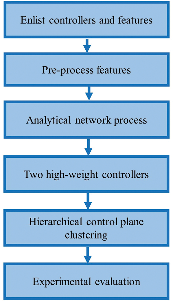
Figure 1: Proposed methodology
3.1 Problem Formulation and System Model
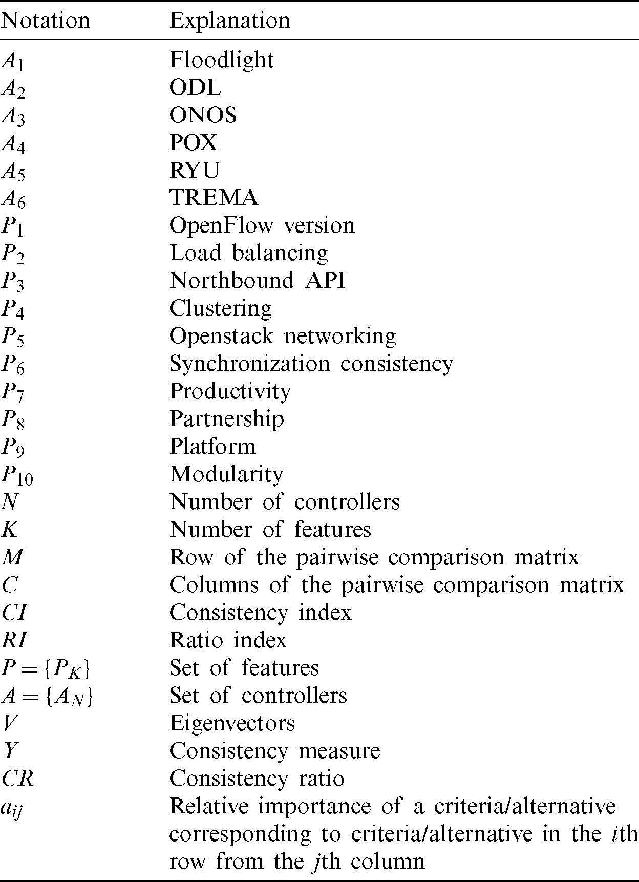
Because there are several controllers, and each controller has multiple features. Hence, the controller selection with multiple features is regarded as a multicriteria-decision-making (MCDM) problem. In this problem, we have to select the controller with a high weight regarding the optimum feature set. Hence, we should rank several controllers regarding their multiple features. Moreover, a single controller is not appropriate for SDN due to SPOF, scalability and performance bottleneck. Consequently, an efficient architecture of multiple controllers in SDN is needed for an improvement in the E2E QoS. To overcome the former problem, we propose an ANP model for ranking the controllers with respect to its features. For the later problem, a HCPC scheme is developed. Eqs. (1) and (2) shows the controllers and their features. Here, controller A1 has features P1, P2,  . An explanation of notations and illustration of Eqs. (1) and (2) are given in Tab. 1.


3.2 Pre-processing of Controller’s Features
Herein, we describe the ten important features that should be considered in an SDN controller with respect to a clustering of the controllers. Hence, we rank the controllers using these ten features by leveraging the ANP tool [27] and conduct an experimental evaluation of the high weight controller in our proposed HCPC environment. We utilize the latest documented information regarding the features of the controller and the studies described in [5–10]. Features of a controller can be categorized into two classes: (1) Ordinal and (2) Regular. Ordinal features support inherent ordering, whereas regular categorical features do not entail such an ordering.
Categorization of the controller features provides a clear vision of the support degree of a feature in a controller. For instance, A4 and A6 only support OpenFlow v1.0. Hence, for this feature (P1), controller is put in a low category (L). Tab. 2 shows each feature and its category. In addition, A1 is placed in a medium (M) category, A2 and A3 support versions, i.e., v1. 0, 1.1, 1.3. Therefore, they are in a high category (H), and A5 supports versions, i.e., 1.5, and therefore is put in a very high (V H) level for this feature. Moreover, P2 denotes the load balancing feature of each controller. Here, Ryu, POX, TREMA, and Floodlight cannot distribute the load evenly because of a lack of coordination among the distributed controllers. Hence, they are placed in the (L) category. In ONOS, the distributed controllers can send message requests among the controllers and hence we place this in the (H) category. However, in ODL, the works are collocated with proper load balancing among the controllers. Hence, this is assigned a (V H) category.
Table 2: Pre-processed features of controllers
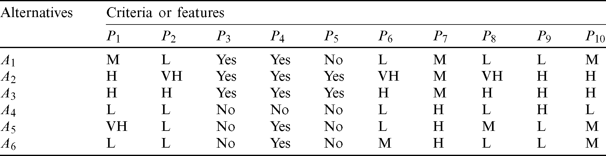
Here, P3, P4, and P5 represents the regular categorical features, i.e., that cannot be divided into more levels. For illustration, a controller can either support REST API or not, clustering, or open stack networking. Consequently, features (P3, P4, and P5) do not entail some inherent ordering. Hence, these are shown with a “Yes” and “No” in Tab. 2. Similarly, A4, A5 and A6 also do not poses support for the REST API; consequently, they are denoted with a “No” in Tab. 2 corresponding to the P3 field. Likewise, A1, A2, and A3 can support REST API; hence a “Yes” is put in column corresponding to P3 which shows the presence of this feature. Moreover, P4 represents a Quantum API support feature, and A1, A2, A3, A5, and A6 have a Quantum API feature support. Consequently, “Yes” is shown in P4 column for them. However, A4 does not support Quantum API, and therefore the column P4 is denoted with a “No” corresponding to the A4 controller. In addition, P5 reveal a clustering feature. As controllers A1, A4, A5, and A6 do not have support for clustering feature; as a result, P5 field is shown with a “No” in Tab. 2. By contrast, A2 and A3 support clustering; thus, they are denoted with a “Yes.”
P6 shows consistency of the synchronization, i.e., denotes the consistency level of the traffic among the distributed data plane managed by multiple controllers. In the case of Ryu, POX is placed in the (L) category and TREMA is placed in the (M) category. ONOS is placed in the (H) category because the information can be altered. The ODL is strongly consistent. As a result, it is placed in the (V H) category. In addition, P7 shows productivity degree for a controller. The productivity denotes the ease for application development. In addition, it is related with the coding language in which controller is programmed. Although Python provides ease for development of applications; however, these controllers are slow due to lack of memory management, deficiency of multi-threading, and absence of platform support across controllers. Moreover, A1, A2, and A3 entail medium productivity, whereas A4, A5, and A6, have high productivity.
In addition, P8 signifies the support of different vendors, whereas A2 has support from NEC, Cisco, Linux foundation, and IBM, the membership of which spans 40 companies; Hence, it is kept in (V H) level. Controller A3 is sponsored by SK Telecom (a South Korea telecommunication company), NEC and Cisco; Consequently, it is in the (H) level. Controllers A1, A4, and A6 are supported by NEC, Big Switch Networks, and Nicira, and hence they are in the (L) level concerning their support. Although vendors support feature is not directly proportional with performance, nevertheless, a high level of support from vendors results in an improvement in performance. Moreover, P9 represents the platform support. Controllers A2, A3, and A4 contains support for Windows, Linux, and Mac, and are therefore placed in (H) class. However, A1, A5, and A6 are entails support for Linux only, and therefore it is assigned an (L) class. The cross-platform feature enables multi-threading and clustering resulting in QoS improvement. Feature P10 shows the support for modularity. Controllers A1, A5, and A6 have a medium modularity level, whereas A2 and A3 have a high-level modularity. The A2 and A3 controllers know how to make a call to sub-functions from the main program, which enable parallel processing and increase the performance. Herein, we apply feature categorization as a pre-processing step.
3.3 SDN Controllers Ranking with ANP
Herein, we describe the ten critical features which should be judged in a controller with respect to a clustering of the controllers. The ANP MCDM problem is formulated by defining the objective, and the parameters (P) (a.k.a) the criteria set, are then defined to evaluate the goal. Finally, a set of alternatives (A) that should be ranked based on the criteria set are identified. Such an approach has widely been used for complex decision-making problems in various fields, i.e., in wireless sensor networks, zone head selection in IoT, node selection for privacy preservation in IoT, and controller placement problems [28–31]. Figs. 2 and 3 show the ANP model created in the Super Decisions simulation tool and the step wise procedure used for ranking the controllers (alternatives) i.e., A1, A2,  for the feature sets P1, P2,
  . The features offered by several controllers are denoted with (P). Moreover, the alternatives are shown with (A) notation. In the subsequent paragraphs, we discuss the procedure for a pairwise comparison of controllers with respect to every feature using an ANP and vice versa.

Figure 2: ANP model for controller ranking

Figure 3: The description of ANP procedure for controllers ranking
3.3.1 Pairwise Comparison for Features and Controllers
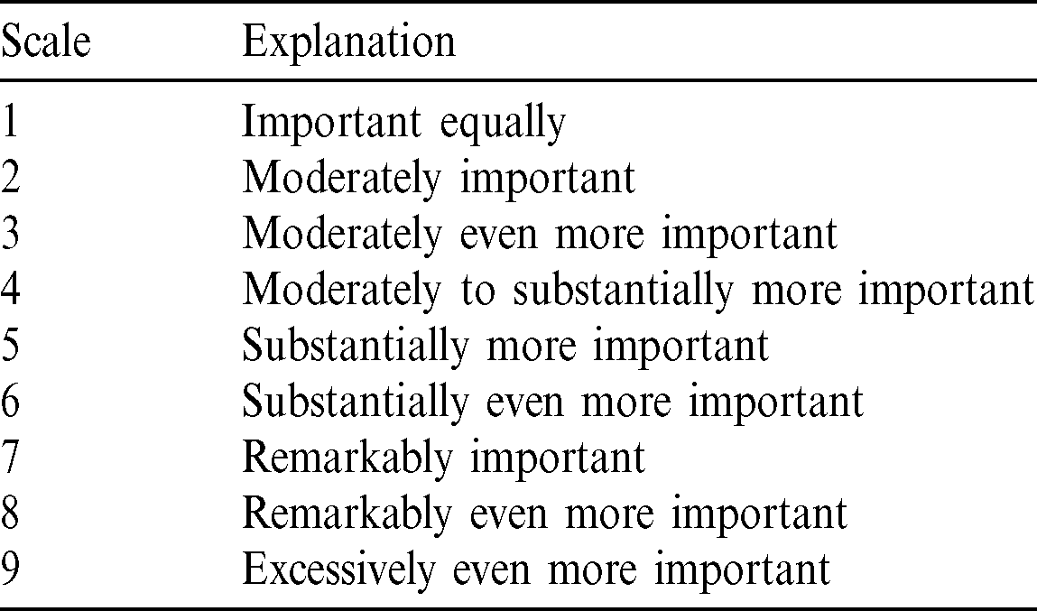
The general form of the pairwise comparison matrix is shown in matrix (3), which is created based on a 9-point scale, as shown in Tab. 3. Controllers are pairwise compared to each feature element, i.e., ten features are applied. The general structure of a pairwise comparison matrix is represented in matrix (3). Matrix (3) shows the rows M1 through Mn and columns C1 through Cn. The value corresponding to a(i, j) signifies the importance of a feature of the ith row versus jth column. Similarly, a(i, j) = 1 in the matrix denotes that P1 feature related to the ith row and jth column controllers is equally present in both controllers. Moreover, diagonal elements represent the comparison of an element with itself; consequently, the values of such elements are denoted by 1, as represented in matrix (4). In addition, the elements values below and above the diagonal are reciprocal of each other. First, alternatives are compared pairwise with respect to the feature P1. The values for elements are included in (3) depending on a 9-point scale, as shown in Tab. 3. The reciprocal and nonreciprocal values show the importance of the row elements from the column components, correspondingly. First, A1 is compared with A2, A3, A4, A5, and A6 considering the P1 criterion. In addition, A1 is of equal importance with itself, and thus a(1, 1) = 1. Then, A2 and A3 are moderately important than A1. Moreover, a(1, 2) = a(1, 3) = 1/3. Here, A1 is moderately important than A4 and A6, e.g., a(1, 6) = 3 shows that the alternative in row (A1) is moderately important than an alternative in the subsequent column (A6). In addition, a(1, 5) = 1/6 reveals that A5 is substantially more important than A1. Likewise, the values are inserted in for A2–A6. In the same way, we meticulously incorporate values for all the elements in matrix (4) for pairwise comparison.
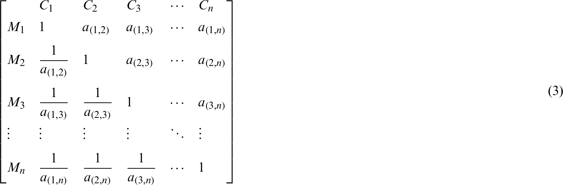

Table 3: Scale for defining the relative importance of a feature and controller
Matrix (5) is then used for the summation, and every value is divided with the summation of a column. Next phase is calculation of an eigenvector, which is computed from a normalized matrix. An eigenvector indicates a priority of the feature (P1). The eigenvector V is obtained from the normalized matrix (6) according to Eq. (7). The result from Eq. (7) is considered as the eigenvector V1, which is shown in (8). To obtain the eigenvector X as shown in Eq. (7), first we compute the normalized matrix (6).


3.3.2 Consistency Index (CI), Consistency Measure (CM), and Consistency Ratio (CR) Calculation
To prove the consistency of the judgments we made during the values insertion in pairwise matrix, the next phase is to compute the consistency index (CI) and consistency ratio (CR). Nevertheless, before evaluating consistency, the vector for consistency measure (CM) should be computed. The calculation of (CM) vector is essential for the computing (CI) and (CR). Eq. (9) shows the procedure for determining the consistency measure. The Mj represents a row from the Eq. (4). Here, V and vi represent the eigenvector and its corresponding component which is also shown in Fig. 4. In addition, the multiplication of Mj and V are taken and then it is divided upon the element in the eigenvector linking to Mj. Fig. 4 shows the procedure used to get (CM). Then, the average of the (CM) vector is taken for computing  max as shown in Eqs. (9) and (10). The procedure to obtain these equations and the overall process is shown in Fig. 4.


Figure 4: Computing the consistency ratio
The CI represents the deviation of comparison matrix for a component. The (CI) for P1 criterion of the matrix is determined using Eq. (11) by applying the value for  . The values of
  , and n = 6 are added in Eq. (11). In Eq. (11), n denotes the number of criteria for the selection of controller in comparison matrix. In this case, six alternatives were put into consideration: hence, n = 6. The final value of (CI) is 0.01 according to Eq. (11).

The trustworthiness of the comparison matrix is verified by means of (CR), which is calculated as given in Eq. (12). In Eq. (12) (RI) represents ratio index. Moreover,  is inserted from Tab. 4, depending upon the matrix order. If rank of a matrix is 3 (number of alternatives for comparison is three), a value relating to 3 is then incorporated for RI. In this example, the criteria elements number is 6. Consequently, a value matching with 6 will be selected from Tab. 4. Then, (CR) is obtained by placing the (CI) from Eq. (11) into Eq. (12). The derived
  , as the
  or less is known for an inconsistent judgment; otherwise, inconsistency is regarded as high. Then, pairwise judgments must be repeated i.e., until the
  . Similarly, for the remaining criteria all the alternatives are compared pairwise, i.e., P2, P3, P4, P5, P6, P7, P8, P9, and P10. Furthermore, the (CR) and (CI) are derived using similar procedure as discussed. Likewise, the eigenvectors corresponding to V1, V2, V3, V4, V5, V6, V7, V8, V9, and V10 are computed corresponding to features P1, P2, P3, P4, P5, P6, P7, P8, P9, and P10, respectively, beside with their values of (CR). Here, V1 illustrates the eigenvector for the P1 criterion. Likewise, V2 denotes the eigenvector of the P2 criterion, V3 represents that for P3, and so on. Similarly, (CR) value for obtaining each eigenvector is proven (which is less than 0.1).


Table 4: Ratio index for different number of criteria

3.3.5 Pairwise Comparison of Criteria (Features) Concerning Alternatives (Controllers)
The ten features P1, P2,  are pairwise compared for all controllers, i.e., A1, A2, A3, A4, A5, and A6. The corresponding eigenvectors for these controllers are then calculated, i.e., V11, V12, V13, V14, V15, and V16 as shown in Tabs. 5 and 6. The eigenvectors for controllers are determined employing similar calculations as applied for the features. Likewise, CM, CI,
  , and CR are determined for all matrices. Further, it is verified that the CR for each eigenvector is less than or equal to 0.10 for maintaining a consistent judgment.
Table 5: Eigenvectors for features with respect to a comparison of the controllers

Table 6: Eigenvectors for controllers with respect to a comparison of features

The eigenvectors are calculated, i.e., denotes the weight for every feature with respect to each controller and vice versa. Next, we represent them in the form of a non-weighted super-matrix. Then, the non-weighted super-matrix is adjusted such that it is column stochastic (total or sum is 1 for each column). The resultant matrix is known as weighted super-matrix, that shows a comparison of the criteria for the alternatives and vice versa. The non-weighted super-matrix is same with weighted super-matrix; but the difference is that the weighted super-matrix poses column stochastic characteristics. Here, V1, V2, V3, V4, V5, V6, V7, V8, V9, and V10 are the eigenvectors corresponding to P1, P2, P3, P4, P5, P6, P7, P8, P9, and P10, which signify of features for each controller. Similarly, V11, V12, V13, V14, V15, and V16 are the eigenvectors corresponding to A1, A2, A3, A4, A5, and A6, which show the priority of the alternatives (controllers) regarding each feature. Tabs. 5 and 6 show the values of the eigenvectors and the consistency ratio from the pairwise comparison matrices and weights obtained from the weighted super-matrix. We can see that the consistency ratio is less than 0.1. Hence, the pairwise matrices are consistent. Lastly, we determine the limit of the super-matrix to find the final weights of the controllers. The computation of which is depicted in next subsection.
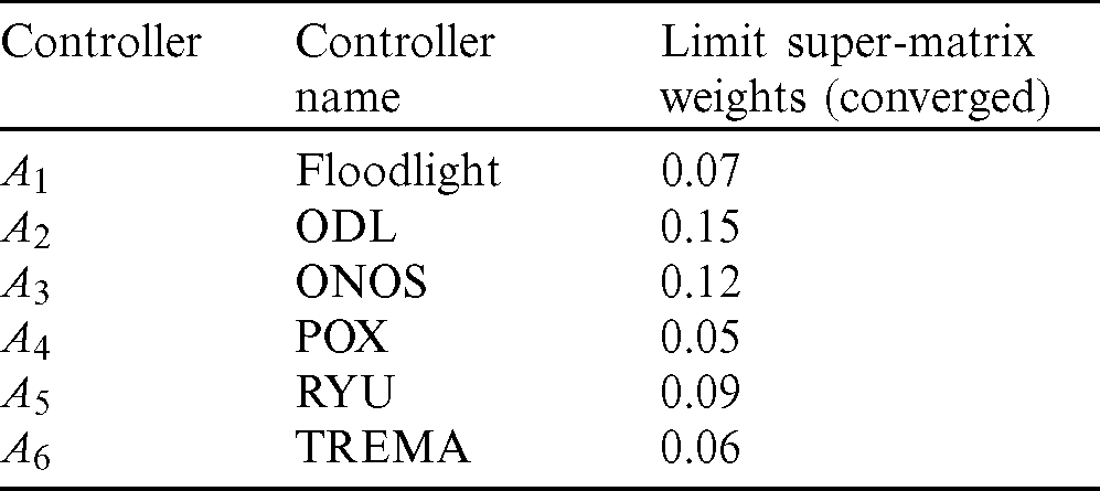
The stable weights are computed by taking the power of the weighted super-matrix continually is continually until we get converged values. A matrix with converged weights is known as a limit super-matrix that reveals the weights of the controllers, i.e., finally prioritized, or converged values. Thus, the limit-matrix comprises of final weights calculated for each controller and feature. This is computed after processing of weighted super-matrix, i.e., the values are raised to the power 2k until all row weights converge, where k shows some random number. The final stable weights of all controllers from the limit super-matrix are shown in Tab. 7. The table shows that A2 has the highest weight; consequently, it signifies the optimal controller. The subsequent appropriate controllers are A3, A5, A1, A6, and A4 respectively, which are arranged according to final weights. Corresponding to these weights, A2 has a high weight, i.e., 0.15, and thus the controller related to it supports the optimum features for the clustering environment, as evaluated with the ANP model. To prove the hypothesis that the controller regarding the optimum features calculated using ANP, in the next section, we evaluate this high weight controllers for an experimental analysis in the HCPC network environment using SDN and make a comparison with DCC approach. Moreover, we also evaluate the runner up controller, i.e., A3.
Table 7: Final weights of controllers through ANP
3.4 Hierarchical Control Plane Clustering for Inter-Domain Collaboration
To enable the inter-domain communication and coordination of tasks among the distributed controllers in each domain, we use an HCP architecture. Fig. 5 depicts the HCP architecture with three inter-communicating domains. In the proposed HCP, there are two layers, i.e., local, and global. The local controller (LC) administers each domain while the global controller (GC) is used for coordination among the local domain controllers. Each domain consists of the data plane network devices, i.e., switches and routers which communicate with the LCs through southbound API.

Figure 5: Efficient hierarchical control plane (HCP) for inter-domain communication
The tasks are delegated from local controllers to the GC in the control plane hierarchy via the northbound API. Consequently, this decreases the computational complexity [32–34]. The hierarchy control plane with a global view reduces the E2E delay when the network devices increases. Moreover, the GC works in a proactive manner. Hence, the global path and state information are available to GC. Consequently, the packets are processed promptly and the E2E resources are provisioned upon arrival of the packets. Fig. 6 shows the communication mechanism in the HCP which is described in algorithm 1.

Figure 6: Communication mechanism in the HCP
3.4.1 Algorithm for Communication Mechanism in the HCP
Algorithm 1 illustrates the communication procedure when a packet arrives from the host (H1) to the switch in a domain. First, the packet header (source and destination) is compared with the source and destination of the flow entries in the switch flow table. If the destination is in the local domain, the switch then sends a Packet-In message to the LC. Then, the local controller returns the path and updates the flow entries on the switch of the domain. By contrast, if the destination of the packet is outside the LC, the LC then forwards the Packet-In packet to the GC, and the GC returns the path to the LC, which updates the flow entries accordingly. However, if the flow entries for the packet already exist on the switch flow table, then the packet is delivered to the destination according to the flow rules already present on the switch. Fig. 6 shows the packets processing in the HCP.

3.4.2 Global Controller Clustering
We make a cluster of the GC in order to combat failures and improve the performance. Hence, we make a cluster of the optimum controller computed with ANP, i.e., ODL and also for the runner up controller, i.e., ONOS. We adopt the clustering mechanism from [22] for the backup of our GC. OpenDaylight allows clustering, which uses a data store that is “sharded.” By default, there are four shards; Topology, Inventory, Normal, and Toaster. Each shard on the network contains all information of a certain sort. The topology shard for instance contains all of the topology details. Only one controller is capable of controlling a given shard and is named its Master. All the others serve as replicas, named Supporters, who must forward requests to the Leader concerned. The Leader will serialize requests and start a three-phase commit process. An action only happens while the commit process is successfully completing the third step. Shards cannot be broken, and the method is fairly consistent since all transactions are serialized. ONOS supports and facilitates clustered execution. It views each controller as a node, where a given node with each device on the network may take on a mastership, backup, or ignored role. For all devices, therefore, there is no imposed single point of contact; leadership of a given device may float between any controller with control connections to that device. Controllers communicate directly and synchronize their state machines every few seconds, gradually making this particular feature consistent; other parts of the system are therefore strongly consistent.
In this section we evaluate the high weight controller calculated with ANP in the proposed HCPC scheme and compare its performance with DCC scheme [26]. First, we describe the experimental setup and the network topology. Then, we leverage an effective network partitioning algorithm for assignment of switches to these controllers. Further, the traffic parameters and performance evaluation results of the two schemes are discussed. Moreover, we also evaluate the runner up controller computed using ANP to validate that the performance improves with the optimum high weight controller. The subsequent subsections describe the details of the experimental approach we will follow.
4.1 Simulation Environment and Comparison
We consider the standard network topology, i.e., Open Science, Scholarship, and Services Exchange (OS3E) [35], also known as an Internet2 network for analysis. We write the Python code with vim editor for the network topology in Mininet [36] emulation platform for an experimental analysis. The Mininet Python API was used for emulating the network on ONOS and ODL controllers. The ONOS and ODL controllers are installed in virtual server machines. The latest Mininet version 2.3.0d1 with Open vSwitch (OVS) version 2.5.4, Ubuntu 16.04 LTS, and Xming server were utilized to originate as well as visualize traffic from source to destination hosts using HCPC and DCC for a comparison of the results. Fig. 7 denotes the proposed HCPC environment that we simulate with ODL and ONOS controllers. The GC is a combination of three controllers i.e., cluster as discussed in Section 3.4.2. We compared our scheme with a DCC [26] approach using a flat controller’s architecture. The authors used multiple controllers distributed in the SDN.

Figure 7: Efficient hierarchical control plane clustering with two level hierarchy (LCs and GC)
4.2 Switches Assignment to the Controllers
The topology is denoted as the graph G = (V, E), where V shows the vertices and E signifies edges of topology. Fig. 8a shows the distribution of V and E in OS3E topology. To assign the switches to the controllers, we leverage an effective algorithm [37] such that the E2E delay between the switches and the controllers in each domain is at minimum. First, we assign switches to the ODL and ONOS controllers placed in each domain. Fig. 8b shows the partitioning of the network topology OS3E and the switches assigned to a controller in each domain. The dotted circles show the switches where the controller is piggybacked, and the solid circles shows the switches in each domain.

Figure 8: The SDN topology for experiments, its partitioning into five domains (a) OS3E topology [35] (b) topology partitioning
4.3 Traffic Generation Parameters
We leverage the distributed Internet traffic generator (D-itg) [38] between the source and destination hosts in the OS3E topology. The step-by-step process for generation of traffic is described in Fig. 9. First, we open a listening socket for the user datagram protocol (UDP) on the destination host (H2) for the traffic originating from other nodes via ITGRecv. A source host (H1), ITGSend is employed to send the UDP traffic with a payload, i.e., 50,000 bytes for a time period of 100 seconds (s) with a constant rate of 50,000 packets/s to destination host with an IP address (192.168.1.2). We repeated the experiment for the OS3E topology 20 times by choosing different source and destination hosts, and the average results for the delay and jitter are obtained.

Figure 9: Traffic generation parameters
4.4 Evaluation of End-to-End Delay
In this experiment, we evaluate the E2E delay for our proposed HCPC and DCC schemes with ODL and ONOS controllers respectively in OS3E topology. Eqs. (14) and (15) show the E2E delay (DPi) calculation procedure using D-itg for the ith packet sent from the source to the destination. Here, SPi and RPi show the transmission and receiving times of a packet P from the source to the destination in OS3E network. Fig. 10 shows the E2E delay for HCPC and DCC approaches. We can see from Fig. 10 that the E2E delay is small for the HCPC as compared to DCC. Moreover, the E2E delay with single controller is more as compared to HCPC and DCC schemes because a single controller creates a performance bottleneck when the number of Packet-In requests towards it increases. Furthermore, the ODL controller with optimal features calculated using the ANP has a smaller E2E delay as compared to ONOS controller. Fig. 10 reveals that the E2E delay with a high ODL controller in a standalone network and in HCPC as well as DCC is small owing to its optimum features (consistency, modularity, fast response of NB and SB APIs) which contribute to the improvement in the QoS.


Figure 10: E2E delay between source and destination hosts with high traffic load
4.5 Evaluation of End-to-End Jitter
During this experiment, we analyze the E2E jitter in the OS3E topology for the ODL and ONOS controllers. The average jitter is obtained using Eq. (16). Fig. 11 shows the E2E jitter for the HCPC and DCC schemes emulated with ODL and ONOS controllers. Fig. 11 reveals that the E2E jitter is smaller in an OS3E network with single and cluster networks with an ODL controller. The ODL controller calculated using ANP has best supported features for the cluster environment. Hence, it results in significantly improving the QoS for both HPCC and DCC mechanisms.


Figure 11: E2E jitter between source and destination hosts with high traffic load
4.6 Evaluation of Load Balancing
In this experiment, we generate background traffic using the hping tool [39] at different speeds, i.e., 100, 200, 300, 400, 500, 600, 700, 800, 900, and 1,000 Mbps. We then inject it into the OS3E topology to evaluate the load balancing performance of the proposed HCPC and DCC schemes with two controllers (ODL and ONOS) obtained using ANP. Fig. 12 shows a comparison of the E2E delay between the source and destination hosts with an increase in the traffic load in the background. We can see from Fig. 12 that the delay with the proposed HCPC is smaller as compared to DCC approach with both ODL and ONOS controllers.

Figure 12: Delay between the source and destination hosts with a variation in the background traffic
Moreover, when using a single controller ODL and ONOS, the E2E delay with ODL controllers is smaller than ONOS with increasing traffic load. This occurs owing to the optimal load balancing features of ODL, i.e., metering provided by OpenFlow and fast response of northbound API, which distribute the load evenly across the nodes between the source and destination.
In this experiment, we analyze the throughput of the proposed HCPC and DCC schemes with high weight controllers, i.e., ODL and ONOS. To evaluate the E2E throughput, we use the Iperf tool [40]. Fig. 13 shows the throughput results obtained through the ODL and ONOS controllers using in HCPC and DCC schemes. We can see from Fig. 13 that the throughput with the ODL controller having the optimum features regarding the clustering is significantly larger than with the ONOS controller in standalone and clusters, i.e., HCPC and DCC approaches. The higher consistency and modularity features of ODL helps in the improved throughput in the standalone and multiple controllers with proposed HCPC and DCC approaches. However, the throughput with optimum ODL controller in proposed HCPC is significantly larger than the throughput in DCC with ONOS controller.

Figure 13: Throughput between source and destination hosts with a high traffic load
4.8 Evaluation of Recovery Time
Fig. 14 shows a comparison of the link failure recovery times (in milliseconds (ms)) for the HCPC and DCC schemes with ODL and ONOS controllers. We create a link failure and observe the recovery time for ODL and ONOS controllers in standalone and cluster environments. The recovery time or total recovery delay (DRtotal) is calculated using Eq. (17) [41]. In Eq. (17) FD denotes failure detection time (ms), PC shows the path calculation time (ms) and FI denotes the flow insertion time (ms). We can see that the recovery time in the HCPC approach is smaller as compared to DCC for both ODL and ONOS controllers. Moreover, the recovery time for ONOS is significantly larger than ODL because ODL supports the latest features which contributes in faster recovery.


Figure 14: Comparison of link failure recovery time
We conducted this experiment to emulate the switches using the Cbench tool [19] for evaluating the throughput of the two high weight controllers obtained through an ANP in HCPC and DCC schemes. We increased the number of switches up to 100 and recorded the throughput, i.e., by sending Packet-In packets to the SDN controllers, ONOS and ODL, respectively in a standalone and cluster environment i.e., HCPC and DCC. The number of MACs per switch is set to 5,000. We send the Packet-In packets to the high weight controllers computed using the ANP. This experiment is repeated 20 times. Fig. 15 shows the results of the throughput with both controllers in a standalone and cluster environment. The results show that the throughput of the ODL controller increases rapidly and maintains the throughput with an increase in switches. Further, the HCPC and DCC improves the QoS of the throughput as compared with a single controller. However, the high weight ODL controller computed using the ANP regarding the cluster-supported features achieves a significant improvement in the throughput as compared to the ONOS in the proposed HCPC scheme.

Figure 15: Throughput evaluation with an increase in the number of switches
The sysbench tool [42] is employed to evaluate the CPU utilization while testing the controllers, i.e., ODL and ONOS computed using the ANP approach amid the traffic generation. Fig. 16 illustrates the CPU utilization results at consecutive intervals of 20 seconds. We can see from Fig. 16 that the utilization does not surpass 30% and 40% amid the peak usage for the runner-up and high weight controllers, i.e., ONOS and ODL, respectively. However, during normal traffic conditions, the CPU utilization does not go beyond 15% for the ONOS controller or 22% for the optimum feature set ODL controller.

Figure 16: CPU utilization of ODL and ONOS controllers amid traffic load
Our study aimed to improve the QoS in SDN using a two step approach i.e., first rank controllers leveraging an ANP based on their features and select a controller with optimum feature set. In the second step, we made the HCPC for SDN to avoid SPOF, performance bottleneck and scalability issues. Moreover, we evaluated the performance of two high weight controllers in a standard OS3E topology using a single controller and our proposed HCPC approach. Further, we compared the results of the two high weight controllers for our proposed HCPC mechanism with a DCC scheme. The experimental results indicate that the controller with a high weight (ODL) in terms of its features outperforms ONOS (with a lesser weight) in two scenarios i.e., when the controller is used without clustering and by applying our proposed HCPC approach and the DCC scheme. The results achieved using the HCPC and DCC prove that the QoS is improved as compared to using a single controller for managing the OS3E network. The experimental results showed that our proposed HCPC approach with an optimum controller (ODL) surpasses the ONOS controller and DCC scheme in terms of the QoS metrics, i.e., the delay, jitter, load balancing, scalability, recovery time and CPU utilization.
Funding Statement: This research was supported by the MSIT (Ministry of Science and ICT), Korea, under the ITRC (Information Technology Research Center) support program (IITP-2020-2018-0-01431) supervised by the IITP (Institute for Information & Communications Technology Planning & Evaluation).
Conflicts of Interest: The authors declare that they have no conflicts of interest to report regarding the present study.
References
1. J. H. Cox, J. Chung, S. Donovan, J. Ivey, R. J. Clark et al. (2017). , “Advancing software-defined networks: A survey,” IEEE Access, vol. 5, pp. 25487–25526.
2. A. A. Barakabitze, A. Ahmad, R. Mijumbi and A. Hines. (2020). “5G network slicing using SDN and NFV: A survey of taxonomy, architectures and future challenges,” Computer Networks, vol. 167, pp. 1–40.
3. A. K. Tran and M. J. Piran. (2019). “SDN controller placement in IoT networks: An optimized submodularity based approach,” Sensors, vol. 19, pp. 1–12.
4. S. Khan, H. A. Khattak, A. Almogren, M. A. Shah, I. Ud Din et al., “5G vehicular network resource management for improving radio access through machine learning,” IEEE Access, vol. 8, pp. 6792–6800.
5. Pox Controller. (2020). Available: https://github.com/noxrepo/pox.
6. Trema Controller. (2020). Available: https://trema.github.io/trema/.
7. Ryu Controller. (2020). Available: https://ryu-sdn.org/.
8. Opendaylight (ODL). (2020). Available: https://www.opendaylight.org/.
9. Floodlight Controller. (2020). Available: https://floodlight.atlassian.net/wiki/spaces/floodlightcontroller/overview.
10. Open Network Operating System (ONOS). (2020). [Online]. Available: https://www.opennetworking.org/onos/. [Google Scholar]
11. S. J. Vaughannichols. (2011). “OpenFlow: The next generation of the network,” Computer, vol. 44, no. 8, pp. 13–15. [Google Scholar]
12. J. Ali, B. H. Roh and S. Lee. (2019). “QoS improvement with an optimum controller selection for software-defined networks,” PLoS One, vol. 14, no. 5, pp. e0217631. [Google Scholar]
13. H. Shiva and C. G.Philip. (2016). “A comparative study on software defined networking controller feature,” International Journal of Innovative Research in Computer and Communication Engineering, vol. 4, pp. 5354–5358. [Google Scholar]
14. V. R. S. Raju. (2018). “SDN controllers comparison,” in Proc. of Science Globe Int. Conf., Bengaluru, India. [Google Scholar]
15. D. Sakellaropoulou. (2017). “A qualitative study of SDN controllers,” . [Online]. Available: https://mm.aueb.gr/master_theses/xylomenos/ Sakellaropoulou_2017.pdf. [Google Scholar]
16. A. A. Semenovykh and O. R. Laponina. (2018). “Comparative analysis of SDN controllers,” International Journal of Open Information Technologies, vol. 6, no. 7, pp. 50–56. [Google Scholar]
17. G. A. Miller. (1956). “The magical number seven, plus or minus two some limits on our capacity for processing information,” Psychological Review, vol. 63, no. 2, pp. 81–97. [Google Scholar]
18. P. Bispo, D. Corujo and R. L. Aguiar. (2017). “A qualitative and quantitative assessment of SDN controllers,” in 2017 Int. Young Engineers Forum (YEF-ECEAlmada, Portugal. [Google Scholar]
19. A. Tootoonchian, S. Gorbunov, Y. Ganjali, M. Casado and R. Sherwood. (2012). “On controller performance in software-defined networks, ” in USENIX Workshop on Hot Topics in Management of Internet, Cloud, and Enterprise Networks and Services (Hot-ICE), USENIX Association 2560 Ninth St. Suite 215 Berkeley, CA, USA. [Google Scholar]
20. R. Khondoker, A. Zaalouk, R. Marx and K. Bayarou. (2014). “Feature-based comparison and selection of software defined networking (SDN) controllers,” in 2014 World Congress on Computer Applications and Information Systems (WCCAISHammamet, Tunisia. [Google Scholar]
21. O. Belkadi and Y. Laaziz. (2017). “A systematic and generic method for choosing a SDN controller,” International Journal of Computer Networks and Communications Security, vol. 5, no. 11, pp. 239–247. [Google Scholar]
22. D. Anderson. (2017). “An investigation into the use of software defined networking controllers in aerial networks,” IEEE Military Communications Conf. (MILCOM), USA, pp. 285–290. [Google Scholar]
23. S. Badotra and S. N. Panda. (2019). “Evaluation and comparison of opendaylight and open networking operating system in software-defined networking,” Cluster Computing, vol. 23, pp. 1–11. [Google Scholar]
24. T. Kim, J. Myung and S. E. Yoo. (2019). “Load balancing of distributed datastore in opendaylight controller cluster,” IEEE Transactions on Network and Service Management, vol. 16, no. 1, pp. 72–83. [Google Scholar]
25. N. Nguyen and T. Kim, “Toward highly scalable load balancing in Kubernetes clusters,” IEEE Communications Magazine, vol. 58, no. 7, pp. 78–83. [Google Scholar]
26. A. Abdelaziz, A. T. Fong, A. Gani, U. Garba, S. Khan et al. (2017). , “Distributed controller clustering in software defined networks,” PLoS One, vol. 12, no. 4, pp. e0174715. [Google Scholar]
27. T. L. Saaty. (2008). “The analytical network process,” Iranian Journal of Operations Research, vol. 1, pp. 1–27. [Google Scholar]
28. H. Farman, H. Javed, B. Jan, J. Ahmad, S. Ali et al. (2017). , “Analytical network process based optimum cluster head selection in wireless sensor network,” PLoS One, vol. 12, no. 7, pp. e0180848. [Google Scholar]
29. H. Farman, B. Jan, H. Javed, N. Ahmad, J. Iqbal et al. (2018). , “Multi-criteria based zone head selection in internet of things based wireless sensor networks,” Future Generation Computer Systems, vol. 87, pp. 364–371. [Google Scholar]
30. H. Farman, B. Jan, Z. Khan and A. Koubaa. (2020). “A smart energy-based source location privacy preservation model for internet of things-based vehicular ad hoc networks,” Transactions on Emerging Telecommunications Technologies, pp. 1–14. [Google Scholar]
31. J. Ali, S. Lee and B. H. Roh. (2019). “Using the analytical network process for controller placement in software defined networks (poster),” in Proc. of the 17th Annual Int. Conf. on Mobile Systems, Applications, and Services (MobiSys ’19New York, NY, USA: Association for Computing Machinery. [Google Scholar]
32. J. Ali and B. H. Roh, “An effective hierarchical control plane for software-defined networks leveraging TOPSIS for end-to-end QoS class-mapping,” IEEE ACCESS, vol. 8, pp. 88990–89006. [Google Scholar]
33. I. Elgendi, K. S. Munasinghe and B. Mcgrath. (2016). “A heterogeneous software defined networking architecture for the tactical edge,” in Proc. of the Military Communications and Information Systems (MilCIS) Conf., Canberra, Australia, pp. 1–7. [Google Scholar]
34. J. Ali and B. Roh. (2019). “A framework for QoS-aware class mapping in multi-domain SDN,” in IEEE 10th Annual Information Technology, Electronics and Mobile Communication Conf. (IEMCONVancouver, BC, Canada, pp. 602–606. [Google Scholar]
35. MRI-R2 Consortium: Development of dynamic network system (DYNES). Available: http://www.internet2.edu/ion/dynes.html. [Google Scholar]
36. R. L. S. De Oliveira, A. A. Shinoda, C. M. Schweitzer and L. R. Prete. (2014). “Using Mininet for emulation and prototyping software-defined networks,” in Proc. of the IEEE Colombian Conf. on Communication and Computing (COLCOMColombia, USA, pp. 1–6. [Google Scholar]
37. G. Wang, Y. Zhao, J. Huang and Y. Wu. (2018). “An effective approach to controller placement in software defined wide area networks,” IEEE Transactions on Network and Service Management, vol. 15, no. 1, pp. 344–355. [Google Scholar]
38. A. Botta, A. Dainotti and A. Pescape. (2012). “A tool for the generation of realistic network workload for emerging networking scenarios,” Computer Networks, vol. 56, no. 15, pp. 3531–3547. [Google Scholar]
39. IPerf. (Accessed on May 2020). Available: https://www.iperf.fr/. [Google Scholar]
40. Hping tool, Accessed May 2020. Available at: https://tools.kali.org/information-gathering/hping3/. [Google Scholar]
41. J. Ali, G. M. Lee, B. H. Roh, D. K. Ryu and G. Park. (2020). “Software-defined networking approaches for link failure recovery: A survey,” Sustainability, vol. 12, pp. 1–28. [Google Scholar]
42. Sysbench tool, Accessed April 2020. Available at: https://github.com/akopytov/sysbench/. [Google Scholar]
 | This work is licensed under a Creative Commons Attribution 4.0 International License, which permits unrestricted use, distribution, and reproduction in any medium, provided the original work is properly cited. |