DOI:10.32604/cmc.2021.014493
| Computers, Materials & Continua DOI:10.32604/cmc.2021.014493 | |
| Article |
Accurate Fault Location Modeling for Parallel Transmission Lines Considering Mutual Effect
1Department of Electrical Engineering, Faculty of Engineering, Assiut University, Assiut, 71518, Egypt
2College of Engineering at Wadi Addawaser, Prince Sattam Bin Abdulaziz University, Al-Kharj, 11911, KSA
3Department of Electrical Engineering, Faculty of Engineering, Minia University, Minia, 61517, Egypt
4Department of Systems Engineering, King Fahd University of Petroleum & Minerals, Dhahran, 31261, KSA
*Corresponding Author: Mujahed Al-Dhaifallah. Email: mujahed@kfupm.edu.sa
Received: 23 September 2020; Accepted: 01 November 2020
Abstract: A new accurate algorithms based on mathematical modeling of two parallel transmissions lines system (TPTLS) as influenced by the mutual effect to determine the fault location is discussed in this work. The distance relay measures the impedance to the fault location which is the positive-sequence. The principle of summation the positive-, negative-, and zero-sequence voltages which equal zero is used to determine the fault location on the TPTLS. Also, the impedance of the transmission line to the fault location is determined. These algorithms are applied to single-line-to-ground (SLG) and double-line-to-ground (DLG) faults. To detect the fault location along the transmission line, its impedance as seen by the distance relay is determined to indicate if the fault is within the relay’s reach area. TPTLS under study are fed from one- and both-ends. A schematic diagrams are obtained for the impedance relays to determine the fault location with high accuracy.
Keywords: New accurate algorithms; mathematical modeling; fault location; scheme diagrams; parallel transmission lines; mutual effect; SLG and DLG faults
An accurate detections of fault location of the high voltage transmission lines (TL) is a critical subject of the researches and engineering for long time. This action explains that a fault point can be resolved extremely not long after a fault happens along a transmission line to save time which is expected to resume the activity of the line and advantage power utilities and customers [1]. An algorithm for fault location dependent on Fourier investigations of a faulted system was proposed [2,3]. The algorithm encapsulates a precise fault location by estimating just nearby end information. Its basic hypothesis was concentrated through computerized recreations on a model force framework. The fault locator has been created in [4,5], which compute the reactance of a flawed line, with a smaller scale processor, utilizing the one-terminal voltage and current information of the transmission line. Another fault location calculation applied to multi-terminal two equal transmission lines was proposed [6–8]. The calculation utilized similar AC contributions as defensive transfers dependent on the greatness of the differential flow at every terminal.
Another strategy for deficiency area estimation was proposed [9,10] utilizing information from the two closures of the TL with no requirement for information synchronization. Two new strategies were proposed for fault location in equal twofold circuit multi-terminal TL by utilizing stage voltages and flows data from CCVT’s and CT’s at every terminal [11–15]. The two strategies were applied to stage to-ground and stage-to-stage flaws. Another issue area strategy dependent on six-sequence fault segments was produced for equal lines dependent on the issue examination of a joint equal TL [16,17]. A calculation for precisely finding TL single line-to-ground flaws with insignificant data of voltage and current was created [18]. A microprocessor-based fault locator was portrayed [19–22], which utilized a novel remuneration strategy to improve precision. An exact fault location method that utilized post-flaw voltage and current determined at both line closes were proposed [23,24]. A fault location technique for one of two exclusively transposed equal transmission lines was depicted [25–30]. Parallel TL under issue were decoupled into the normal part net and differential segment net [31–35]. Ground fault area of TL dependent on time contrast of appearance of ground-mode and airborne mode voyaging waves was examined in [36–38].
In this research work, a new accurate algorithm based on mathematical modeling of two parallel transmissions lines system (TPTLS) as influenced by the mutual effect to determine the fault location is discussed. The distance relay measures the impedance to the fault location which is the positive-sequence. The principle of summation the positive-, negative-, and zero-sequence voltages which equal zero, of Ef1 +Ef2 +Ef0 = 0, is used to determine the fault location on the TPTLS. Also, the impedance of the transmission line to the fault location is determined. These algorithms are applied to single-line-to-ground (SLG) and double-line-to-ground (DLG) faults. To detect the fault location along the transmission line, its impedance as seen by the distance relay is determined which indicates if the fault within the reach of the relay. TPTLS under study are fed from one- and both-ends. A schematic diagrams are obtained for the impedance relays to determine the fault location with high accuracy.
2 Mathematical Modeling of TPTLS Fed on One-End
Fig. 1 shows a two parallel transmission lines system (TPTLS) TL1 and TL2, which are protected by two distance relays R at bus 1. Where; If: fault current; IB: line current from bus 1; EB1: bus voltage at bus 1; It: total current fed from the generator at bus 1.

Figure 1: Two parallel transmission lines system (TPTLS) fed on one-end
2.1 Determination of the Fault Location without Mutual Coupling between TPTLS
Fig. 2 shows the sequence impedance networks of SLG fault occurred at one-line of the TPTLS at percentage (fraction) n of the line length where, the sequence networks are connected in series in SLG fault to determine the fault currents as:


where, IB0, IB1, and IB2: Zero-, positive-, and negative-sequence currents at bus 1; It0, It1, and It2: Zero-, positive-, and negative-sequence total current fed from the generator at bus-1.

where, n: percentage (fraction) of line length that is location of fault has happen. From Eq. (3) the bus sequence currents are equal, i.e.,

Because It1 = It2 = It0.

Figure 2: (A) Equivalent positive-, (B) Equivalent negative-, and (C) Equivalent zero-sequence networks of parallel transmission line systems fed from one-end without taking into account the mutual effect
At bus 1, the voltage sequence-components EB1 is:

The generator G voltage (emf)  pu.
pu.

The voltage at fault location Ef is:

From Fig. 2:


Adding Eqs. (8)–(10) and using Eqs. (4), (6) and (7) to obtain:

From Eq. (11), n(cal): calculated percentage (fraction) of line length is:

where,

Therefore, the impedance of the transmission line to fault location ZR which measured by the distance relay is:

Fig. 3 shows a schematic diagram of the distance relay that determine the fault location on the faulted TL based on the TL impedance ZR which indicates if the fault is within the relay’s reach area.

Figure 3: The schematic diagram for the implementation of the impedance relay
Fig. 2 shows the sequence impedance networks of DLG fault occurred at one-line of the TPTLS at percentage (fraction) n of the line length where, the sequence networks are connected in parallel in DLG fault to determine the fault currents as:

Again; IB0, IB1, and IB2: Zero-, positive-, and negative-sequence currents at bus 1; It0, It1, and It2: Zero-, positive-, and negative-sequence total current fed from the generator at bus 1. Eq. (3) can be applied in this case and the voltage sequence-components EB1 at bus 1 is calculated as:

The generator G voltage (emf)  pu.
pu.

The voltage at fault location Ef is:

In analogy with Eqs. (8)–(10), a three similar equations can be written:


where,

where;  and
and  : total (equivalent) impedances of the zero- and negative-sequence networks without the mutual effect, respectively.


Adding Eqs. (19), (22) and (23), and using Eqs. (17) and (18), one can write:

Eq. (24) can be written in another form:

where,

Eq. (25) is a cubic complex coefficients equation:

Solving this equation, Eq. (26), using MATLAB software to determine the calculated percentage (fraction) n(cal), which expresses where the fault is located, (n(cal) is the real one of three solutions). Therefore, the impedance of the transmission line to fault location ZR which measured by the distance relay is:

Fig. 4 shows a schematic diagram of the distance relay that determine the fault location on the faulted TL based on the TL impedance ZR which indicates if the fault is within the relay’s reach area.

Figure 4: The schematic diagram for the implementation of the impedance relay
2.2 Determination of Fault Location of TPTLS as Affected by Mutual Coupling
Fig. 5 shows the sequence impedance networks of SLG fault occurred at one-line of the TPTLS at percentage (fraction) n of the line length where with mutual effect between TPTLS.

Their components Itm1 = Ifm1 = IBm1, Itm2 = Ifm2 = I and Itm0 = Ifm0 = IBm0:

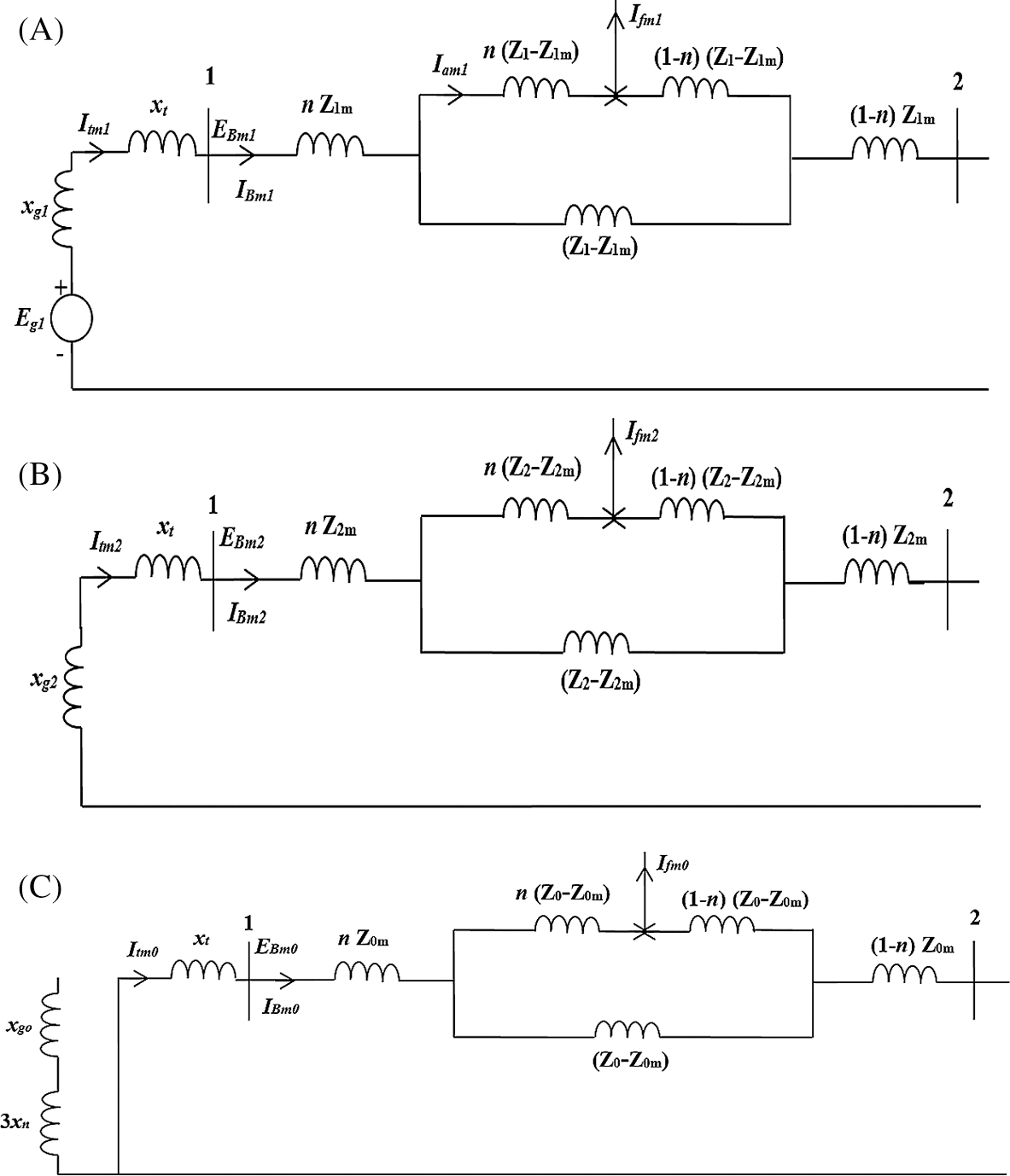
Figure 5: (A) Equivalent positive-, (B) equivalent negative-, and (C) equivalent zero-sequence networks of TPTLS fed from one-end taking into account the mutual effect
From Eqs. (28) and (29) the bus sequence currents are equal, i.e.,

The voltages at fault location Efm and at the bus location EBm are:


With reference to Fig. 5, one can write:


where, Z1m, Z2m, and Z0m: The positive-, negative- and zero-sequence mutual impedances between the parallel TL. Adding Eqs. (33)–(35), and using Eqs. (29)–(32) to obtain:

where, Zm = Z1m +Z2m +Z0m. The solution of the quadratic Eq. (36) determines the calculated percentage (fraction) nm(cal) as:

Therefore, the distance relay can measure the impedance ZRm which is expressed as:

where,  : the current of n(Z1 − Z1m) branch. Fig. 6 shows a schematic diagram of the distance relay that determine the fault location on the faulted TL based on the TL impedance ZRm which indicates if the fault is within the relay’s reach area.

Figure 6: The schematic diagram for the implementation of the impedance relay
Fig. 5 shows the sequence impedance networks of DLG fault occurred at one-line of the TPTLS at percentage (fraction) n of the line length with mutual effect.

Their components Itm1 = Ifm1 = IBm1, Itm2 = Ifm2 = IBm2 and Itm0 = Ifm0 = IBm0. The voltage sequence-components EBm at bus 1 is calculated as:

The generator G voltage (emf)  pu.
pu.

The voltage at fault location Efm is:

In analogy with Eqs. (8)–(10), a three similar equations can be written with aid of Fig. 5.


where,
where;  and
and  : total (equivalent) impedances of the zero- and negative-sequence networks with taking into account the mutual effect, respectively.


Adding Eqs. (43), (46) and (47), and using Eqs. (41) and (42), one can write:
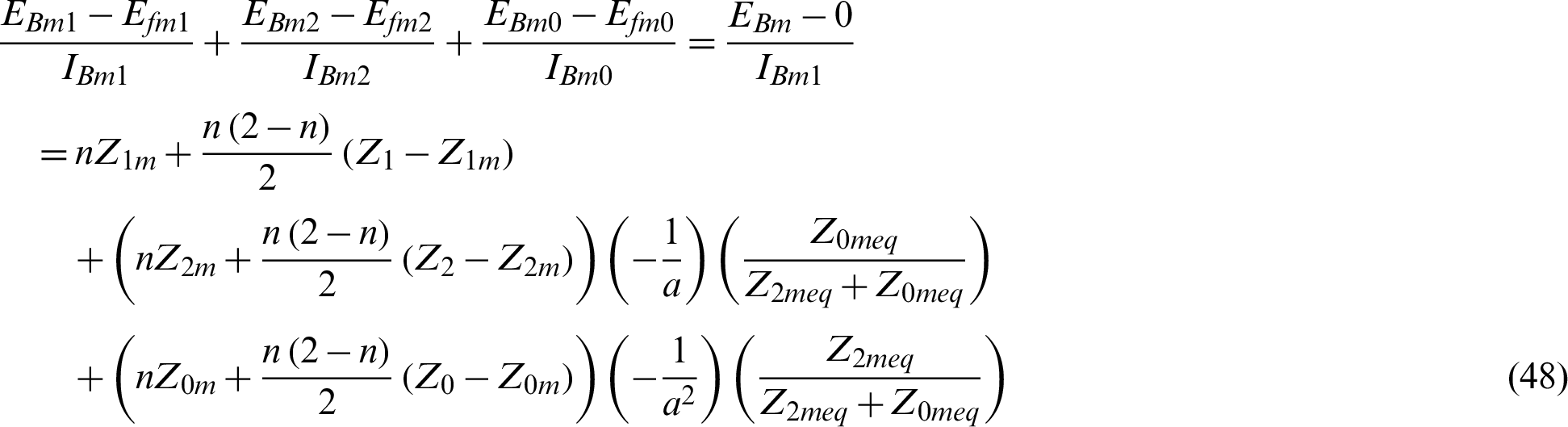
Eq. (48) can be written in another form:

where,

Eq. (49) represents a fourth-order equation with complex coefficients:

where,

Solving this equation, Eq. (50), using MATLAB software to determine the calculated percentage (fraction) nm(cal), which expresses where the fault is located (nm(cal) is the real one of the four solutions). Therefore, the distance relay can measure the impedance ZRm which is expressed as:

where Iam1 is the current that passes through n(Z1 − Z1m) branch. The schematic diagram for the implementation of the impedance relay is as shown in Fig. 7, which determine the fault location on the faulted TL based on the TL impedance ZRm which indicates if the fault is within the relay’s reach area.

Figure 7: The schematic diagram for the implementation of the impedance relay
3 Mathematical Modeling of TPTLS Fed on Both-Ends
Fig. 8 shows a two parallel transmission lines system (TPTLS) TL1 and TL2, which are protected by two distance relays R at bus-1. Where; If: fault current; IB: line current from bus-1; EB1, EB2: bus voltages at bus-1 and bus-2 respectively; It1, It2: total currents fed from the generators G1 at bus-1 and G2 at bus-2.

Figure 8: The two parallel transmission lines system (TPTLS) fed on both-ends
3.1 Determination of Fault Location Without Mutual Coupling Between TPTLS
Fig. 9 shows the sequence impedance networks of SLG fault occurred at one-line of the TPTLS at percentage (fraction) n of line length with taking into account the mutual effect. The delta connection of the parallel TL converted to star connection for simplifying the circuit. Fig. 10 shows the positive-sequence network after such conversion.


Figure 9: (A) Equivalent positive-, (B) equivalent negative-, and (C) equivalent zero-sequence networks of parallel transmission line systems fed from both-ends without taking into account the mutual effect

Figure 10: Delta-to-star conversion of positive-sequence network
The total current It which supplied from generator G1 at bus-1 are:

The current sequence-components IB which supplied from generator G1 (Appendix A) are:

The voltage sequence-components EB at bus-1 are:

where, the emf of generators G1 and G2 are ( ) pu.
) pu.

The fault voltage sequence-components Ef are:

where their sum is equal to zero, i.e.,

In analogy with Eqs. (8)–(10), a three similar equations can be written with aiding of Fig. 9. Adding these equations and using Eqs. (57) and (59), one can write:

where, CF: compensating factor which is expressed as:

So, the calculated percentage (fraction) n(cal) which is a define of fault location on the TL:

And, the measured impedance that seen by the relay ZR is:

Fig. 11 shows a schematic diagram of the distance relay that determine the fault location on the faulted TL based on the TL impedance ZR which indicates if the fault is within the relay’s reach area.

Figure 11: The schematic diagram for the implementation of the impedance relay
3.2 Determination of Fault Location with Mutual Coupling of TPTLS
Fig. 12 shows the total (equivalent) sequence impedance networks, positive- negative- and zero-sequence networks, of TPTLS at percentage (fraction) n of the line length with mutual effect. The delta connection of the parallel TL converted to star connection for simplifying the circuit. Fig. 13 shows the positive-sequence network after such conversion.


Figure 12: (A) Equivalent positive-, (B) equivalent negative-, and (C) equivalent zero-sequence networks of parallel transmission line systems fed from both-ends with mutual effect

Figure 13: Delta-to-star conversion of the positive-sequence network
The total current Itm components which supplied from generator G1 at bus-1 are:

The sequence components of the current in the branch n(Z1 − Z1m), n(Z2 − Z2m), and n(Z0 − Z0m) in Fig. 12, respectively (see Appendix A) are:

The voltage-sequence components EB at bus-1 are:


where the emf of generators G1 and G2 are ( ) pu. The sequence components of the voltage at the fault Ef are:

where their sum is zero, i.e.,:

In analogy with Eqs. (8)–(10), a three similar equations can be written with aiding of Fig. 13. Adding these equations and using Eqs. (69) and (71), one can write:

where, CFm: compensating factor which is expressed as:

Eq. (72) representing the total (sum) impedances between fault location and the bus-1 which is re-expressed as:

where,

Eq. (74) represents a cubic complex coefficients equation:

where,


Solving this equation, Eq. (75), using MATLAB software to determine the calculated percentage (fraction) nm(cal), which expresses where the fault is located, (nm(cal) is the real one of the four solutions). Therefore, the distance relay can measure the impedance ZRm which is expressed as:

where,  is the current of n(Z1 − Z1m) branch. The schematic diagram for the implementation of the impedance relay is as shown in Fig. 14 that determine the fault location on the faulted TL based on the TL impedance ZRm which indicates if the fault is within the relay’s reach area.

Figure 14: The schematic diagram for the implementation of the impedance relay
A MATLAB code is applied to the strategy which is explained before in Sections 2 and 3 to decide the percentage (fractions) n(cal) and nm(cal) characterizing the fault location of two parallel transmission lines system (TPTLS) with or without taking into account the mutual coupling between the parallel lines. The positive-sequence impedances ZR and ZRm which seen by the distance relay R are determined at various places of the fault. This makes it conceivable to decide the relay under-reach at proportion for various positions of the fault. SLG and DLG faults are examined when the system is fed from one- or both-ends.
For SLG faults, the proposed algorithms can determine exactly where the location of the fault whatever the system is fed from one- or both-ends and with or without mutual coupling between the TPTLS as listed in Tabs. 1–4. Also, the proposed algorithms are worked well in case of DLG faults fed from one- or both-ends and with or without mutual coupling between the TPTLS as listed in Tabs. 5 and 6.
Table 1: Calculated fault location n(cal) and nm(cal) seen by distance relay ZR and ZRm, and reach–ratio for SLG faults with and without mutual effect of one-end systems

Table 2: Calculated fault location n(cal), nm(cal), zero-sequence impedances Z0R and  , and ratio (
 ) for SLG faults with mutual effect of one-end systems

Table 3: Calculated fault location n(cal) and nm(cal) seen by distance relay ZR and ZRm, and reach-ratio for SLG faults with and without mutual effect of both-end systems

Table 4: Calculated fault location n(cal), nm(cal), zero-sequence impedances Z0R and  , and ratio (
 ) for SLG faults with and without mutual effect of both-end systems
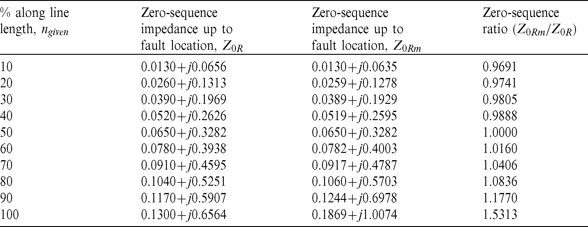
Table 5: Calculated fault location n(cal) and nm(cal) seen by distance relay ZR and ZRm, and reach-ratio for DLG faults with and without mutual effect of one-end systems

Table 6: Calculated fault location n(cal), nm(cal), zero-sequence impedances Z0R and  , and ratio (
 ) for DLG faults with and without mutual effect of one-end systems

From Tabs. 1, 3 and 5, the calculated values of percentage (fraction) n(cal) and nm(cal) that obtained from the proposed algorithms are exactly equal to the ngiven which is defining the fault location on one-faulted TL of the TPTLS.
In one-end systems, the impedance relay is under-reach due the mutual coupling between the TPTLS, ZRm is less than ZR and the reach-ratio is given in negative values in Tabs. 1 and 3 while in systems fed from both-ends, the reach-ratio is positive close to bus-1 and negative values for far faults from bus-1, Tabs. 3 and 4.
Fig. 15A shows that the relay R can see currents flowing in the same direction of  of systems that feeds from one-end. Therefore, the line impedance that seen by the relay ZR is small. In Fig. 15B the faults accrue far away from bus-1, so the current passes through long section of TL,
  and the increase of mutual coupling is more noticeable in the relay ZRm, over ZR. This is why reach-ratio values are small for faults close to bus-1 and increased while increasing the distance of faults far away from bus-1, Tabs. 1, 3 and 5. Not only the impedance is seen by the relay, but also the zero-sequence impedance
  exceeds Z0R, the impedance without mutual coupling as given in Tabs. 2, 4, and 6.

Figure 15: The flowing currents in the TPTLS fed from one-end for (A) near-bus fault, and (B) far-bus fault on
Fig. 16A shows the relay that can see currents in the opposite direction of a-f1 portion for faults close to bus-1 in systems fed from both-ends. ZRm exceeds ZR which mean the relay is overreach or positive-value as listed in Tab. 3 without considering the mutual coupling between the TPTLS. Fig. 16B shows that as fault moves far away from bus-1, the relay can see the current that flowing in the longer portion a-f2 of the faulted line. So, ZRm is less than ZR, which mean reach ratio is negative without taking into account the effect of mutual coupling as listed in Tab. 3. In the case of fault occurred at the mid-way of the faulted line length, the relay will not be in over- or under-reach in Tabs. 3 and 4, Fig. 16C.

Figure 16: The flowing currents in the TPTLS fed from both-end for (A) near-bus fault, (B) far-bus fault, and (C) mid-way fault on
Fig. 17 shows that the zero-sequence ratio ( ) for SLG faults increases at the fault moves along the line length toward the far-bus. This is simply explained by the increasing effect of the mutual coupling between parallel lines. The zero-sequence ratio for DLG faults is almost the same as for SLG faults in Fig. 17.

Figure 17: Zero-sequence ratio for SLG and DLG faults against fault location ngiven
Based on mathematical computation of the fault location of parallel transmission lines with taking into account the effect of mutual coupling between parallel lines, the conclusions can be listed as:
• An accurate algorithms of determination of fault location on parallel transmission lines fed from one- or both-ends with or without considering the mutual coupling is considered in details of the research work. These algorithms are applied to SLG and DLG faults occurred on one of the paralleled transmission lines.
• The impedances that the distance relay sees with or without mutual coupling in one- or both-ends feeding systems in SLG or DLG faults are calculated.
• A schematic diagrams of the proposed algorithms are obtained based on the mathematical modeling of fault location which indicates if the fault is within the relay reach area.
Funding Statement: The authors received no specific funding for this study.
Conflicts of Interest: The authors declare that they have no conflicts of interest to report regarding the present study.
References
1. R. Godse and S. Bhat. (2020). “Mathematical morphology-based feature-extraction technique for detection and classification of faults on power transmission line,” IEEE Access, vol. 8, pp. 38459–38471.
2. Z. Wang, X. Ma, Y. Lu, C. Wang, X. Lin et al. (2020). , “Single-ended data based fault location method for multi-branch distribution network,” Energy Reports, vol. 6, no. 2, pp. 385–390.
3. T. Takagi, Y. Yamakoshi, J. Baba, K. Uemura and T. Sakaguchi. (1981). “A new algorithm of an accurate fault location for EHV/UHV transmission lines,” IEEE Transactions on Power Apparatus and Systems, vol. PAS-100, no. 3, pp. 1316–1323.
4. F. Zhang, Q. Liu, Y. Liu, N. Tong, S. Chen et al. (2020). , “Novel fault location method for power systems based on attention mechanism and double structure GRU neural network,” IEEE Access, vol. 8, pp. 75237–75248.
5. C. Pritchard, T. Hensler, J. Coronel and D. Gachuz. (2016). “Test and analysis of protection behavior on parallel lines with mutual coupling,” in Proc. IEEE PES Transmission & Distribution Conference and Exposition-Latin America (PES T&D-LA20–24 September, Morelia, Mexico.
6. T. Nagasawa, M. Abe, N. Otsuzuki, T. Emura, Y. Jikihara et al. (1992). , “Development of a new fault location algorithm for multi-terminal two parallel transmission lines,” IEEE Transactions on Power Delivery, vol. 7, no. 3, pp. 1516–1532.
7. J. L. Blackburn. (1993). Symmetrical Components for Power Systems Engineering, 1 ed. New York, USA: Marcel Dekker, Inc.
8. M. M. Saha, J. Izykowski and E. Rosolowski. (2010). Fault Location on Power Networks. London Limited, London, UK: Springer-Verlag.
9. T. Funabashi, H. Otoguro, Y. Mizuma, L. Dube and A. Ametani. (2000). “Digital fault location for parallel double-circuit multi-terminal transmission lines,” IEEE Transactions on Power Delivery, vol. 15, no. 2, pp. 531–537.
10. H. X. Ha, B. H. Zhang and Z. L. Lv. (2003). “A novel principle of single-ended fault location technique for EHV transmission lines,” IEEE Transactions on Power Delivery, vol. 18, no. 4, pp. 1147–1151. [Google Scholar]
11. S. M. Brahma. (2005). “Fault location scheme for a multi-terminal transmission line using synchronized voltage measurements,” IEEE Transactions on Power Delivery, vol. 20, no. 2, pp. 1325–1331. [Google Scholar]
12. C. Fan, H. Cai and W. Yu. (2005). “Application of six-sequence fault components in fault location for joint parallel transmission line,” Tsinghua Science and Technology, vol. 10, no. 2, pp. 247–253. [Google Scholar]
13. G. Richards and O. Tan. (1982). “An accurate fault location estimator for transmission lines,” IEEE Transactions on Power Apparatus and Systems, vol. PAS-101, no. 4, pp. 945–950. [Google Scholar]
14. J. Izykowski, R. Molag, E. Rosolowski and M. M. Saha. (2006). “Accurate location of faults on power transmission lines with use of two-end unsynchronized measurements,” IEEE Transactions on Power Delivery, vol. 21, no. 2, pp. 627–633. [Google Scholar]
15. S. H. Kang, Y. J. Ahn, Y. C. Kang and S. R. Nam. (2009). “A fault location algorithm based on circuit analysis for untransposed parallel transmission lines,” IEEE Transactions on Power Delivery, vol. 24, no. 4, pp. 1850–1856. [Google Scholar]
16. L. Eriksson, G. D. Rockefeller and M. M. Saha. (1985). “An accurate fault locator with compensation for apparent reactance in the fault resistance resulting from remote-end infeed,” IEEE Transcations on Power Apparatus and Systems, vol. 104, no. 2, pp. 424–436. [Google Scholar]
17. C. A. Apostolopoulos and G. N. Korres. (2012). “Accurate fault location algorithm for double-circuit series compensated lines using a limited number of two-end synchronised measurements,” International Journal of Electrical Power & Energy Systems, vol. 42, no. 1, pp. 495–507. [Google Scholar]
18. B. Mahamedi, J. G. Zhu, S. Azizi and M. Sanaye-Pasand. (2015). “Unsynchronised fault location technique for three-terminal lines,” IET Generation, Transmission & Distribution, vol. 9, no. 15, pp. 2099–2107. [Google Scholar]
19. A. T. Johns and S. Jamali. (1990). “Accurate fault location technique for power transmission lines,” IEE Proceedings C (Generation, Transmission and Distribution), vol. 137, no. 6, pp. 395–402. [Google Scholar]
20. R. Razzaghi, G. Lugrin, H. M. Manesh, C. Romero, M. Paolone et al. (2013). , “An efficient method based on the electromagnetic time reversal to locate faults in power networks,” IEEE Transactions on Power Delivery, vol. 28, no. 3, pp. 1663–1673. [Google Scholar]
21. L. B. Shenga and S. Elangovan. (1999). “A fault location method for parallel transmission lines,” International Journal of Electrical Power & Energy Systems, vol. 21, no. 4, pp. 253–259. [Google Scholar]
22. Brahma S. M. (2006). “New fault-location method for a single multi-terminal transmission line using synchronised phasor measurements,” IEEE Transactions on Power Delivery, vol. 21, no. 3, pp. 1148–1153. [Google Scholar]
23. S. Jiale, S. Guobing, X. Qingqiang and C. Qin. (2006). “Time-domain fault location algorithm for parallel transmission lines using unsynchronized currents,” International Journal of Electrical Power & Energy Systems, vol. 28, no. 4, pp. 253–260. [Google Scholar]
24. C. Y. Evrenosoglu and A. Abur. (2005). “Travelling wave based fault location for teed circuits,” IEEE Transactions on Power Delivery, vol. 20, no. 2, pp. 1115–1121. [Google Scholar]
25. H. A. Ziedan and H. H. El-Tamaly. (2007). “Fault current calculations as influenced by the mutual effect between parallel lines,” Electric Power Components and Systems, vol. 35, no. 9, pp. 1007–1025. [Google Scholar]
26. W. D. Stevenson. (1955). Elements of Power System Analysis. 1 ed., New York, USA: McGraw-Hill International Book Company, pp. 241–259. [Google Scholar]
27. F. D. Silva and C. L. Bak. (2017). “Distance protection of multiple-circuit shared tower transmission lines with different voltages–-Part II: Fault loop impedance,” IET Generation, Transmission & Distribution, vol. 11, no. 10, pp. 2626–2632. [Google Scholar]
28. R. Liang, Z. Yang, N. Peng, C. Liu and F. Zare. (2017). “Asynchronous fault location in transmission lines considering accurate variation of the ground-mode traveling wave velocity,” Energies, vol. 10, pp. 1957. [Google Scholar]
29. Y. Zhang, Q. Zhang, W. Song, Y. Yu and X. Li. (2000). “Transmission line fault location for double phase-to-earth fault on non-direct-ground neutral system,” IEEE Transactions on Power Delivery, vol. 15, no. 2, pp. 520–524. [Google Scholar]
30. K. Yu, J. Zeng, X. Zeng, F. Xu, Y. Ye et al. (2020). , “A novel traveling wave fault location method for transmission network based on directed tree model and linear fitting,” IEEE Access, vol. 8, pp. 122610–122625. [Google Scholar]
31. C. Zhang, G. Song, T. Wang and L. Yang. (2019). “Single-ended traveling wave fault location method in DC transmission line based on wave front information,” IEEE Transactions on Power Delivery, vol. 34, no. 5, pp. 2028–2038. [Google Scholar]
32. Y. Q. Chen, O. Fink and G. Sansavini. (2018). “Combined fault location and classification for power transmission lines fault diagnosis with integrated feature extraction,” IEEE Transactions on Industrial Electronics, vol. 65, no. 1, pp. 561–569. [Google Scholar]
33. R. Salat and S. Osowski. (2004). “Accurate fault location in the power transmission line using support vector machine approach,” IEEE Transactions on Power Systems, vol. 19, no. 2, pp. 979–986. [Google Scholar]
34. T. Takagi, Y. Yamakoshi, M. Yamaura, R. Kondou and T. Matsushima. (1982). “Development of a new type fault locator using the one-terminal voltage and current data,” IEEE Transactions on Power Apparatus and Systems, vol. PAS-101, no. 8, pp. 2892–2898. [Google Scholar]
35. D. Novosel, D. G. Hart, E. Udren and J. Garitty. (1996). “Unsynchronized two-terminal fault location estimation,” IEEE Transactions on Power Delivery, vol. 11, no. 1, pp. 130–138. [Google Scholar]
36. S. D. Santo and C. M. Pereira. (2015). “Fault location method applied to transmission lines of general configuration,” International Journal of Electrical Power & Energy Systems, vol. 69, pp. 287–294. [Google Scholar]
37. C. Fei, G. Qi and C. Li. (2018). “Fault location on high voltage transmission line by applying support vector regression with fault signal amplitudes,” Electric Power Systems Research, vol. 160, pp. 173–179. [Google Scholar]
38. S. Hussain and A. H. Osman. (2016). “Fault location scheme for multi-terminal transmission lines using unsynchronized measurements,” International Journal of Electrical Power & Energy Systems, vol. 78, pp. 277–284. [Google Scholar]
Appendix A.
Bus currents as a function of fault current and total current supplied to bus 1. Concerning Fig. A1, one can write:

So,

Similarly,


Figure A1: Positive-sequence network
 | This work is licensed under a Creative Commons Attribution 4.0 International License,, which permits unrestricted use, distribution, and reproduction in any medium, provided the original work is properly cited. |