Computers, Materials & Continua DOI:10.32604/cmc.2021.014221
Article

Meenu Gupta1, Rachna Jain2, Simrann Arora2, Akash Gupta2, Mazhar Javed Awan3, Gopal Chaudhary2,*and Haitham Nobanee4,5,6

1Chandigarh University, Punjab, India
2Bharati Vidyapeeth’s College of Engineering, New Delhi, India
3Department of Software Engineering, University of Management and Technology, Lahore, Pakistan
4Collage of Business, Abu Dhabi University, Abu Dhabi, United Arab Emirates
5Oxford Center for Islamic Studies, The University of Oxford, Oxford, UK
6Management School, The University of Liverpool, Liverpool, UK
*Corresponding Author: Gopal Chaudhary. Email: gopal.chaudhary88@gmail.com
Received: 07 September 2020; Accepted: 12 November 2020

Abstract: The COVID-19 disease has already spread to more than 213 countries and territories with infected (confirmed) cases of more than 27 million people throughout the world so far, while the numbers keep increasing. In India, this deadly disease was first detected on January 30, 2020, in a student of Kerala who returned from Wuhan. Because of India’s high population density, different cultures, and diversity, it is a good idea to have a separate analysis of each state. Hence, this paper focuses on the comprehensive analysis of the effect of COVID-19 on Indian states and Union Territories and the development of a regression model to predict the number of discharge patients and deaths in each state. The performance of the proposed prediction framework is determined by using three machine learning regression algorithms, namely Polynomial Regression (PR), Decision Tree Regression, and Random Forest (RF) Regression. The results show a comparative analysis of the states and union territories having more than 1000 cases, and the trained model is validated by testing it on further dates. The performance is evaluated using the RMSE metrics. The results show that the Polynomial Regression with an RMSE value of 0.08, shows the best performance in the prediction of the discharged patients. In contrast, in the case of prediction of deaths, Random Forest with a value of 0.14, shows a better performance than other techniques.

Keywords: COVID-19; state-wise analysis; discharges and deaths; SARS CoV-2; root mean square error

1  Introduction

India witnessed its first case of COVID-19 on January 30, 2020, and the cases were further increased by February 3, 2020 [1]. In February, there was not so much increase in the Corona cases in the country. The first death from this virus in India happened in Karnataka, where the victim was an older man of 76 years who came from Saudi Arabia [2]. The infection of this virus spread in India due to people who came from abroad. All those who had recent travel history were advised to be quarantined. But due to the negligence of some people, this virus spread across the country today. A Sikh minister that came back from moving to Italy and Germany, conveying the infection, transformed into “super spreader” by going to a Sikh celebration in Anandpur Sahib during March [3,4]. Twenty-seven COVID-19 cases were followed back to him. Over 40,000 individuals in 20 towns in Punjab were isolated on March 27 to contain the spread [5]. On March 31, a Tablighi Jamaat strict gathering occasion that occurred in Delhi in early March rose as another virus hotspot. Various cases across the country were followed back to the event [6].

India is the most densely populated country in the world. Along with this, the technology and medical facilities are also not so much advanced. For this reason, preventing this virus was a very big challenge in this country. Many steps have been taken to stop the rise in the number of cases of corona affected people in India. Thermal screening tests of every passenger who came from abroad, especially China was started, and those who founded with high fever were sent to the isolations [7]. Over March, multiple states across the country began to shut down schools, colleges, public facilities such as malls, gyms, cinema halls, and other public places. On March 22, the Government of India imposed a complete lockdown for 21 days in 82 districts of 22 states and union territories [8]. The growth rate of the pandemic had slowed to one of doubling every six days, from a rate of doubling every three days earlier. Due to which the lockdown period is increased three times (first till May 3, then till May 17, and finally till May 31). People are advised to follow social distancing and follow all the precautions during the lockdown period. As of June 3, there are 207615 confirmed cases of COVID-19 across the country. From which 100,303 have been recovered, and 5,815 casualties occur [9]. Half of the cases are reported from only six cities, i.e., Mumbai, Delhi, Ahmedabad, Chennai, Pune, and Kolkata [10,11].

Since most of the research and articles focus on the total deaths and infected patients of entire India altogether, but because of India’s high population density, different cultures, and diversity, it is good to have a separate analysis of each state of India. Hence, in this paper, we seek to carry out a comparative analysis of the prediction of an increase in recovered. Death cases in different states and union territories in India in the near future, as predicting these cases, would help estimate and arrange beds, ventilators, and other healthcare equipment on time and save many lives with proper facilities. This work uses three Machine learning regression algorithms; Polynomial Regression, Decision Tree Regression, and Random Forest Regression. The data is taken from the mohfw.gov.in website. The metric used is Root Mean Square Error (RMSE) for determining accuracy.

The rest of the paper is organized as follows: Section 2 describes the various researches done in the world related to the Corona Virus. Section 3 discusses the methodology, which includes data processing and the different algorithms used. Section 4 reports the experimental results and analysis. Section 5 concludes the research done and suggests future areas of study.

2  Literature Survey

Today, the world is grappling with Corona (COVID-19) Virus [12]. It all started from Wuhan city of China on December 31, 2019 [13], and it spread all over the world very quickly and has become a public health threat [14]. On March 11, 2020, the WHO declared the virus outbreak a pandemic. The virus causes various symptoms, including cough, cold, fever, and, in more severe cases, difficulty breathing [15]. There are approximately 5,675,271 total cases of COVID-19 recorded throughout the world until May 26, 2020. Among which 2,286,305 get recovered, and 356,993 died due to this deadly disease. Men were more infected with this deathly disease than women as determined by a study, and there is no death among children because of this disease [16].

Poon et al. [17] proposed the research to develop the early diagnosis test for COVID-19 by using viral RNA extraction methods and real-time PCR technology. For the result, 50 NPA abbreviated as nasopharyngeal aspirate, samples are taken. And the study shows that the early predictions of COVID-19 in the human body are highly increased with high precision by combing the RNA extraction method with PCR technology [17]. Singh et al. proposed a SIR model that is age-structured, with social contact matrices extracted from Bayesian imputations and surveys to study the COVID-19 progress in India. The age disposition, social contact framework, and data from cases have been used to calculate the procreative ratio and its generalization dependent on time [18].

Qin et al. worked on the Dysregulation of the immune feedback, mainly the T lymphocytes that might have played a significant role in the spread of COVID-19. The data of all the examinations, which include peripheral lymphocyte subset, were studied, and a comparison was made between severe and other patients [19]. Further, Deb et al. [20] proposed a time series framework to evaluate the incidence framework’s pattern and trends. The model is compact and using the right diagnostic methods. The authors showed that a quadratic trend dependent on time captures the incident disease pattern [20]. Murugesan et al. analyzed the spatial dissemination and swings by using the GIS software, which would help in monitoring the virus dispersing problem [21]. Fanelli et al. worked on analyzing the transient dynamics of the COVID-19 disease in China, Italy, and France from January 22 till March 15. The model positions the outbreak in Italy near March 21 with a maximum number of infected individuals near 26000 (not even including recovered and deceased). The number of fatalities at the end of the epidemic is 18,000 [22].

Caruso et al. worked on the analysis of patients suspected with COVID-19 and respiratory symptoms, and the criterion used for exclusion was chest CT scans [23]. Fontanet et al. conducted a reflective closed study among people and their relatives, where a questionnaire was to be filled, which covered the history of fever and respiratory syndromes since January 13 and blood tests for anti-SARS-CoV-2 antibodies [24]. Magal et al. predicted the cumulative count of cases that were reported to a certain size. The main features of the model were the implementation time of public policies, the identification of not reported cases, their isolation, and the impact of asymptomatic cases [25]. Ghosh et al. worked on the various Indian states having a high number of COVID-19 cases. They constructed three growth models for predicting future COVID-19 affected cases along with the recovery rate by using preventive measures [26]. Das et al. proposed a model known as epidemiological SIR for the state-wise prediction of basic reproduction number R0. They also tried to implement a model for the upcoming case prediction. According to their research, the value of R0 for the nation comes out to be 2.75 (March 4, 2020), which is very similar to the Hubei province in their early diagnosis stage. The R0 value for Punjab is calculated around 16, which is too high and hence needs the most attention to focus upon [27].

The limitations that can be inferred from the previous works is that various inconsistent evidence is used for prediction as in some cases CT scan images are used, in other cases viral RNA and immune feedbacks are used for prediction purpose, which ultimately causes inconsistency in the results obtained through supervised learning models. After discussing the various researches, this study is focused on the analysis and predictions of total discharge and total death cases of COVID-19 in different states of India in the future. Different regression algorithms have been applied for the study. This work is in consideration of people’s health and to make them aware of how precaution can save their life where the enemy is in front of you but hidden.

3  Methodology

For analyzing the impact of COVID-19 in different places of India, the dataset is collected from the trusted source; after obtaining the dataset, different regression algorithms are applied, which are discussed below.

3.1 Data Used

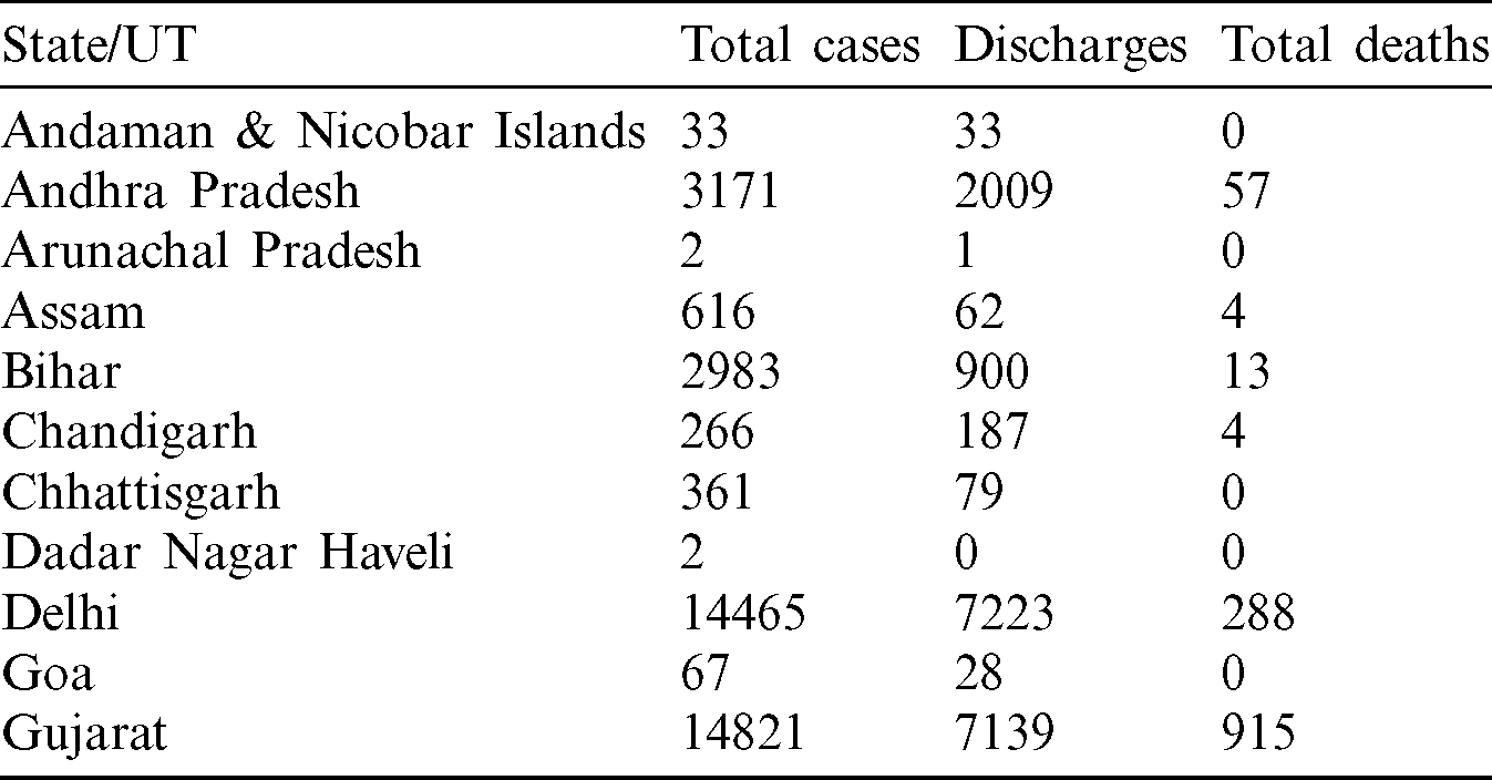
The data used for this research is taken from two websites COVID19 India [28] and the Government of India’s website [29]. The dataset provided the total cases, total discharges, and total deaths that occur due to COVID-19 in each state and union territory of India till May 28, 2020. Tab. 1 represents the sample of the dataset used in this research.

Table 1: Sample dataset

3.2 Algorithms Used

In this paper, three regression models, namely, Polynomial Regression, Decision Tree Regression, and Random Forest Regression, are used to analyze the effect of COVID-19 on various Indian states and Union Territories, along with the prediction of the number of discharged patients and death cases in these states.

3.2.1 Polynomial Regression (PR)

It is a unique circumstance of linear regression in which we align the data with a curvilinear correlation between the target variable and the independent variables in a polynomial equation. This type of regression gives better results when we have an association in data that is not linear and helps plot the best fit curve, which gives the minimum squared error [30]. Polynomial Regression is also useful when we want an extensive range of functions and curvatures for the prediction model [31].

Steps to build a PR model:

The steps to build a polynomial regressor are shown below in Eqs. (1) and (2).

I. Forming the hypothesis function

where, .

II. Minimizing the cost function

where, J () represents the cost function, n is the degree of the polynomial, h (x(i)) is the actual value, and y(i) is the predicted value. Here, represents the regularization parameter, and w stands for the coefficients.

Fig. 1, represents the total cases vs. total discharges and total deaths curves, respectively, by utilizing the Polynomial Regression model.

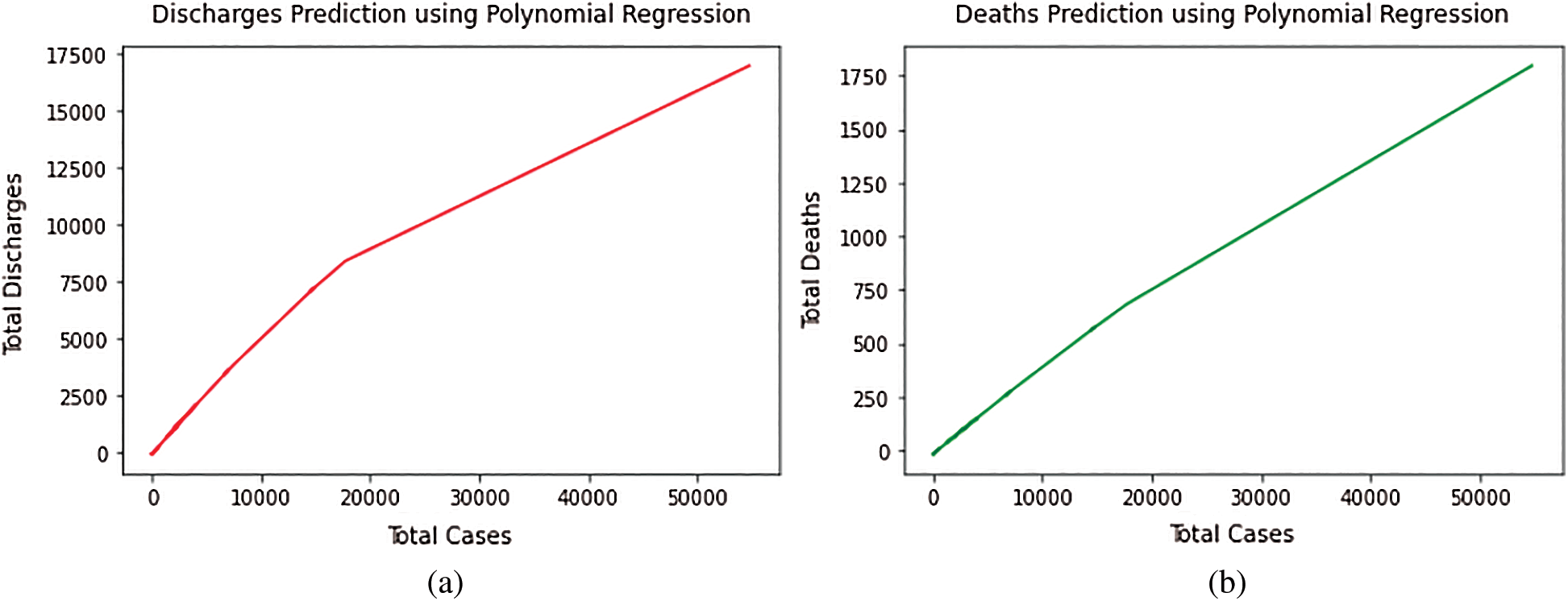
Figure 1: (a) Total discharges prediction using polynomial regression model. (b) Total deaths prediction using polynomial regression model

3.2.2 Decision Tree Regression (DTR)

A DT regressor is an algorithm that is based on the concept of supervised machine learning. A Decision tree resembles a flow-chart structure, where the internal nodes denote a check over an attribute, each branch depicts the result of a test, and each terminal node shows carries along with it a class label. This model, based on our input data, learns a set of questions to figure out the class labels. For the determination of splits, in this case, we use the mean squared error metrics as we have continuously varying data in regression problems. The model is depicted in Fig. 2, given below.

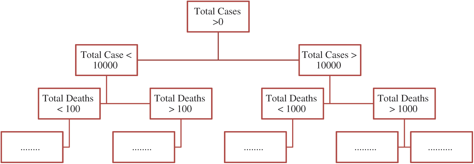
Figure 2: Decision tree regression model

The decision tree algorithm shows good performance in managing tabular data along with numerical characteristics or categorical characteristics with those far less from over a hundred categories. Apart from linear models, they can acquire variation interaction between the features and the target. Fig. 3 represents the total cases vs. total discharges and total deaths curves, respectively, by utilizing the Decision Tree Regression model.

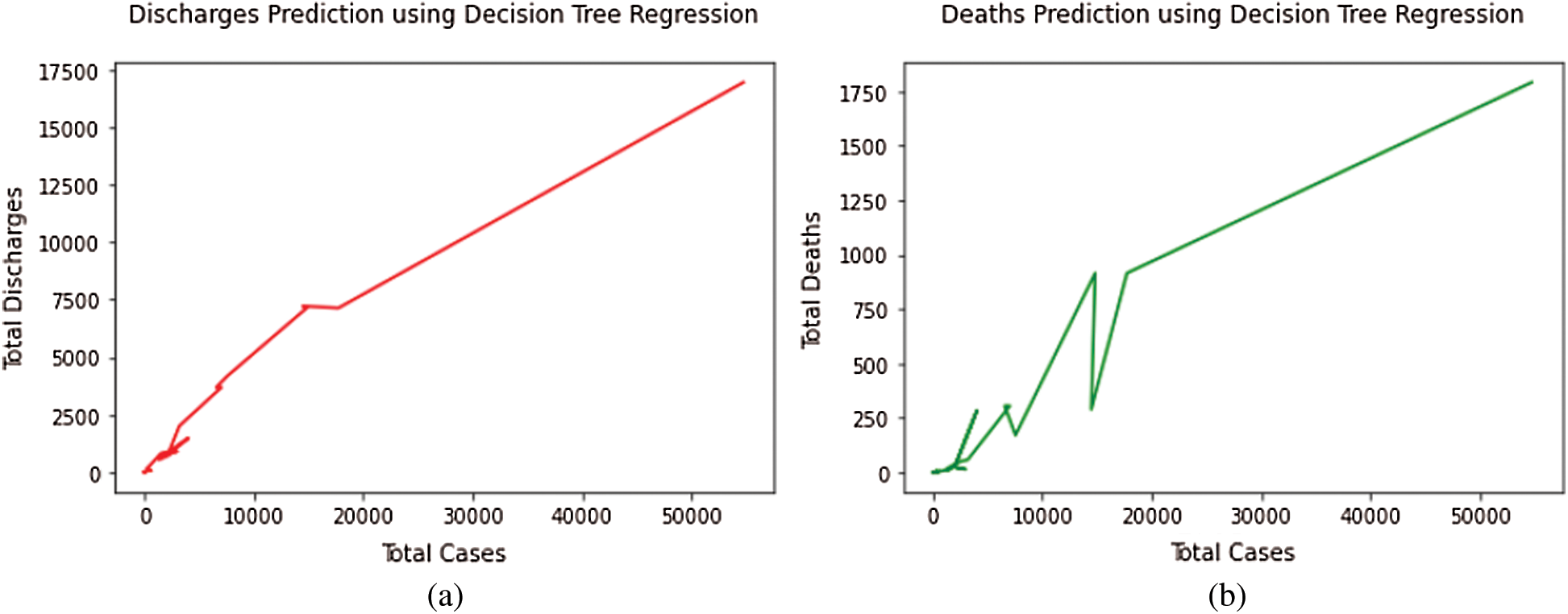
Figure 3: (a) Total discharges prediction using decision tree regression model. (b) Total deaths prediction using decision tree regression model

3.2.3 Random Forest Regression (RFR)

A Random Forest is a type of model that uses an ensemble approach to give good prediction results. It is one of the methods used to conduct both regression and classification tasks with the use of multiple decision trees and a technique known as Bootstrap Aggregation, or bagging for the same [32,33]. The basic idea behind this algorithm is to combine different decision trees and come to final output for better results. The mathematical formulation for the model is shown below in Eq. (3).

where h(x) is known as the summation of base models, and the output is an ensemble of these models, which are at the root level, various decision tree models only. The tree is formed in Decision trees by specifying the important variables as nodes, but in the case of Random Forest, arbitrariness is added to the model as the tree grows. This model also helps in saving time as very little time is spent in hyper-parameter tuning in this case. Fig. 4 represents the total cases vs. total discharges and total deaths curves, respectively, by utilizing the Random Forest Regression model.

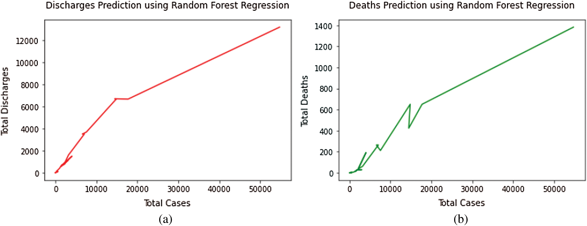
Figure 4: (a) Total discharges prediction using random forest regression model. (b) Total deaths prediction using random forest regression model

3.3 Proposed Model

The proposed model is illustrated in Fig. 5. Initially, the data related to total discharges and total death cases in every State and Union Territory of India are provided as an input to the model.

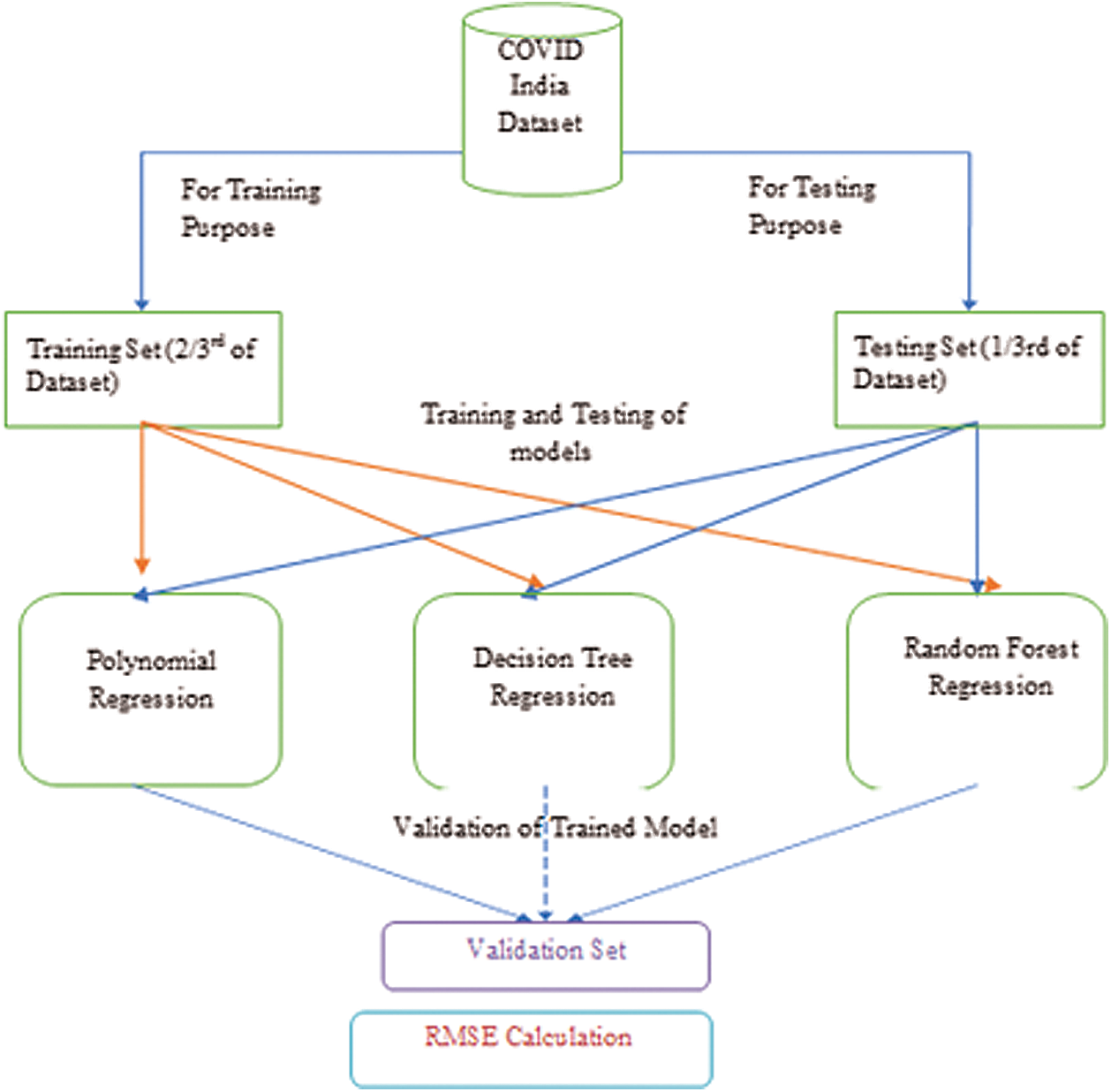
Figure 5: A proposed model using various regression algorithms

In the model, 33% of the dataset is used for testing purposes and remaining for the training purpose. After this, different regression techniques are applied to compare the results based on the RMSE values and to predict the best algorithm for the future scenario.

4  Experimental Result Analysis

This work witness a comprehensive analysis of the COVID-19 Outbreaks across various Indian states and Union Territories. As the COVID-19 cases are on a surge in India, it becomes the need of the hour to analyze the deaths, infected, and recovered cases in various states and predict them using the machine learning models. Different regression models are applied in this study and are further discussed in the subsections using the evaluation metrics.

4.1 Evaluation Metrics

The evaluation metrics used in this work are Mean Squared Error (MSE) and Root Mean Squared Error (RMSE). These are discussed in detail below:

4.1.1 Mean Squared Error (MSE)

It is obtained by calculating the mean of squares, which is the difference between the initial sample data and the approximate values taken [34]. This error depicts the effectiveness of the regression line, and the smaller value of MSE error illustrates that the fit is better as the magnitude of error is minimal. Eq. (4) represents the error function below:

where N is the total number of observations, Yi is the actual value, and is defined as a predicted value. The difference between them is calculated, squared, and the summation is performed over them to achieve the final loss [35].

4.1.2 Root Mean Squared Error (RMSE)

The normal distribution of residuals (prediction errors) is the Root Mean Square Error (RMSE). Residuals are a measure of how far these data points are from the regression line, and it is a measure of how those residuals are spread out [36]. Eq. (5) depicts this error:

where N is the total number of observations, Yi is the actual value, and is defined as a predicted value. The difference between them is calculated, squared, and the summation is performed to achieve the final loss [37]. Finally, the root is taken over this while calculating the accuracy.

4.2 State Wise Analysis

The virus spreads from other creatures to humans. The COVID-19 and the human coronaviruses are categorized in the family of Coronaviridae [38]. India, a nation of 135 crore people, has reported more than 1.5 lakhs confirmed COVID-19 cases after around four months from January 30, 2020, from the first reported case of a student returned from Wuhan in Kerala, among which 65,578, i.e., approximately 30% of the COVID-19 patients were cured or discharged. Around 2% of people died due to this deadly disease in India. The collective prevalence of COVID-19 is swiftly growing day by day [39]. The benchmarking, besides the estimation of analytical representations for COVID-19, is not an inconsequential process [40]. The comparison of the total number of deaths with the total number of discharges throughout India is represented in Fig. 6.

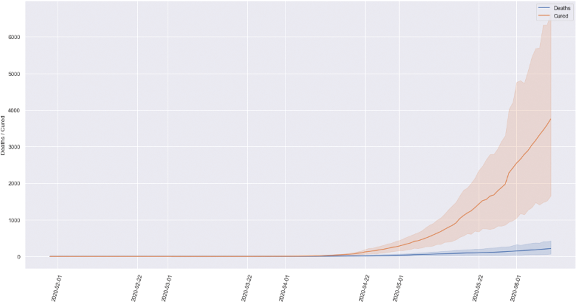
Figure 6: Comparison of the total number of deaths and discharges

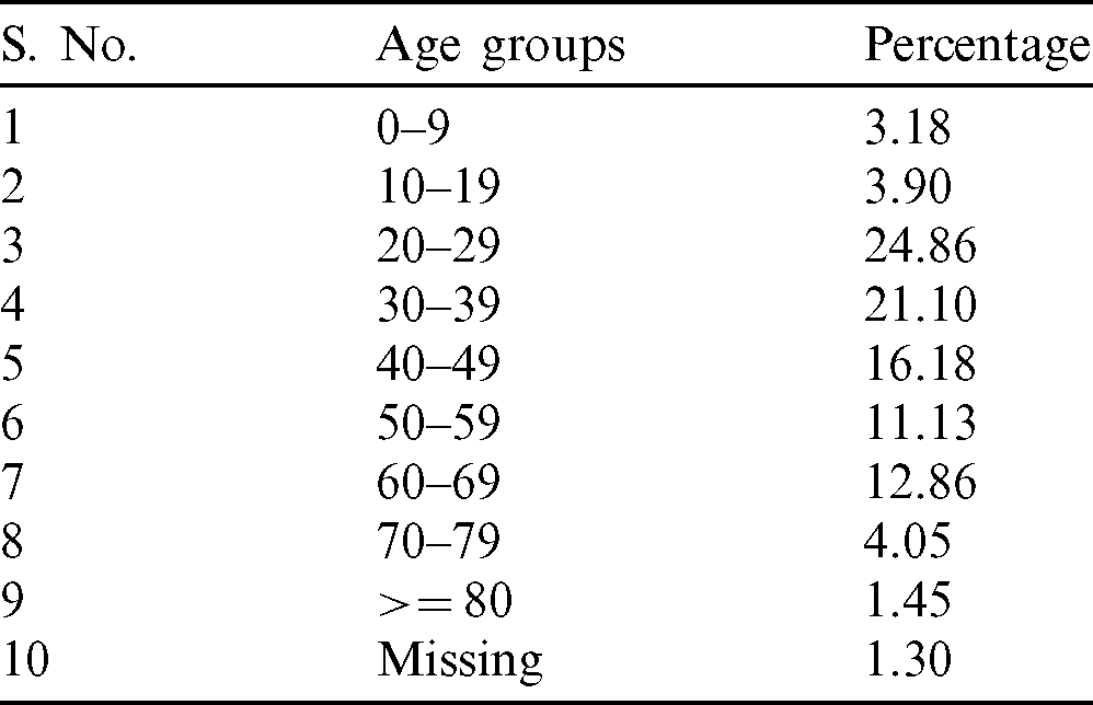
Tab. 2 shows the statistics of total deaths distribution among various age-groups. The analysis also shows that more than 50% of COVID-19 deaths in India have occurred in the 20–49 age groups–-the most economically productive ones. This is an alarming situation as the youth or the working class of the country is highly vulnerable to this disease.

Table 2: Total deaths distribution among various age groups

Hence, because of different population density, Government rules and regulations, and various cultures, considering India’s entire page is not right. Therefore, we analyze India’s states and union territories, having more than 1000 cases of COVID-19 till May 28, 2020. The analysis of total infected, deaths and discharged patients along with the mortality and recovery rate analysis of all the Indian states and Union territories is carried out as follows:

4.2.1 Total Infected Cases Analysis

Fig. 7 represents the total infected cases of all the seventeen states and union territories having more than 1000 COVID-19 cases. It is evident that Maharashtra has 54,758, i.e., the highest number of COVID-19 cases in India. Even after three phases of the lockdown, the state has not seen any decline in increasing infected patients. The rapid spread of this virus can also be accounted for as many infected people are also not showing symptoms or developing symptoms after quite a long time, leading to a greater transmission rate. After Maharashtra, Tamil Nadu shows the highest number of infected cases, i.e., 17,728. Tamil Nadu is one of the states where the lockdown effects can be observed from the beginning to the April end. However, there is an increasing trend observed in May. After Tamil Nadu, Gujarat has recorded 14,821 cases till May 28, 2020. As the Tamil Nadu, Gujarat also shows exponential growth in the latter part of the lockdown. After that, Delhi has recorded 14,465 infected cases so far, which is very close to Gujarat. Although Delhi is the most densely populated city in India, most of the cases were recorded in the past few days only. Due to high population density, it is a matter of concern since the spread of the virus is much easier in such cities.

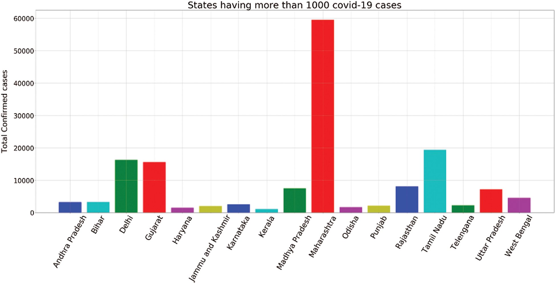
Figure 7: States having more than 1000 infected cases

After that, Rajasthan, Madhya Pradesh, and Uttar Pradesh have recorded 7536, 7024, and 6548 cases, respectively. The COVID-19 situation is not controlled yet in these states and will show tremendous growth in the COVID-19 cases in the latter part of lockdown.

4.2.2 Total Discharges Analysis

Fig. 8 represents the total discharge cases of all the seventeen states and union territories, which records more than 1000 COVID-19 cases.

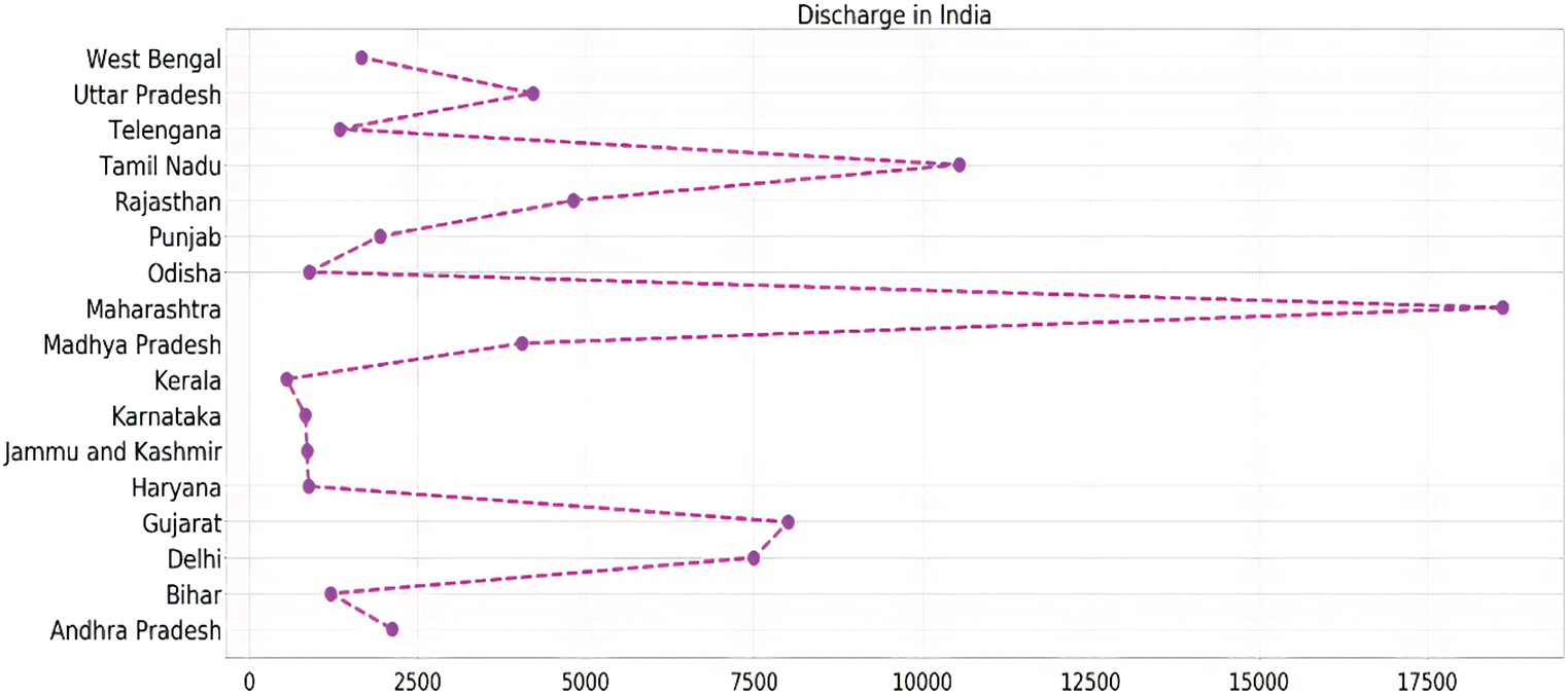
Figure 8: State-wise analysis of total discharge in India

Although in most of the states, the discharge to infected ration remains almost similar, there are some states which show a high release to the infected ratio, which represents that they are in the right direction to control the spread of this deadly pandemic. Mostly, the southern states of the countries, including Tamil Nadu, Kerala, and Telangana, showed such a good ratio.

4.2.3 Total Deaths Analysis

Fig. 9 represents the total death cases of all the seventeen states and union territories, which records more than 1000 COVID-19 cases. West Bengal and Gujarat show the highest death to infected ratio among all the countries of 0.07 and 0.06, respectively, which represents the seriousness of the disease in these countries. Besides these, most of the states like Madhya Pradesh, Maharashtra, Telangana, and Uttar Pradesh having nominal death to infected ratios. Andhra Pradesh, Delhi, and Karnataka reported a lower number of fatalities than these countries. Bihar, Kerala, Odisha, and Tamil Nadu show the lowest deaths in the country that proves that they are in the right direction to control the spread of this deadly pandemic.

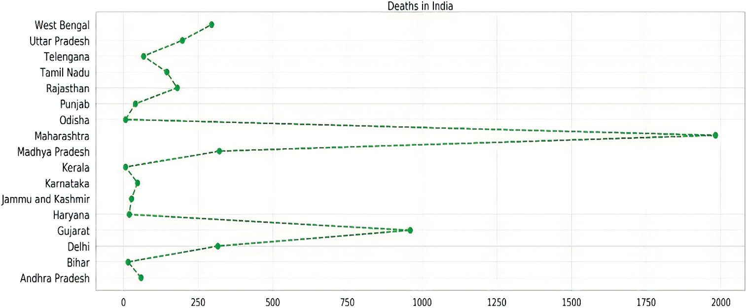
Figure 9: State-wise analysis of total deaths in India

4.2.4 Mortality and Recovery Rate Analysis

The mortality rate of various Indian states and union territories are represented in Fig. 10.

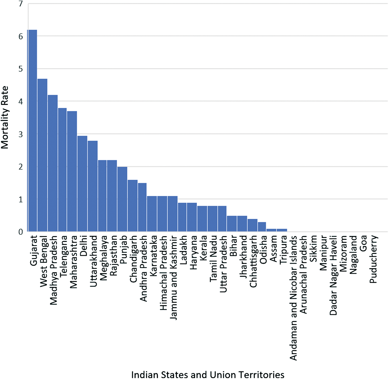
Figure 10: Mortality rate of Indian states and union territories

Fig. 10 shows that the mortality rate in Gujarat is extremely high as compared to other states and union territories, followed by West Bengal and then Madhya Pradesh. This is because the testing rates are quite low in these states, and also, people are not reporting to the hospitals on time. On the other hand, some states like Goa and northeastern states like Manipur, Mizoram, Nagaland, and Sikkim have practically zero mortality rate. This is due to a low population density in these states, and testing and reporting few cases at the right time have further helped in controlling the spread of the virus to a great extent in these areas.

The recovery rate of various Indian states and union territories are represented in Fig. 11. It shows that the recovery rate is higher in Andaman and Nicobar Islands, which is followed by Chandigarh and, subsequently, other states. This is due to the low population density in these areas, which led to high testing and cure of the infected persons. We can also see that the recovery rate is almost zero in states like Sikkim and very low in Mizoram, Arunachal Pradesh, and Nagaland. This is because there are not many cases in northeastern states, and hence the recovery rate is almost nil in these states as not many people are getting infected.

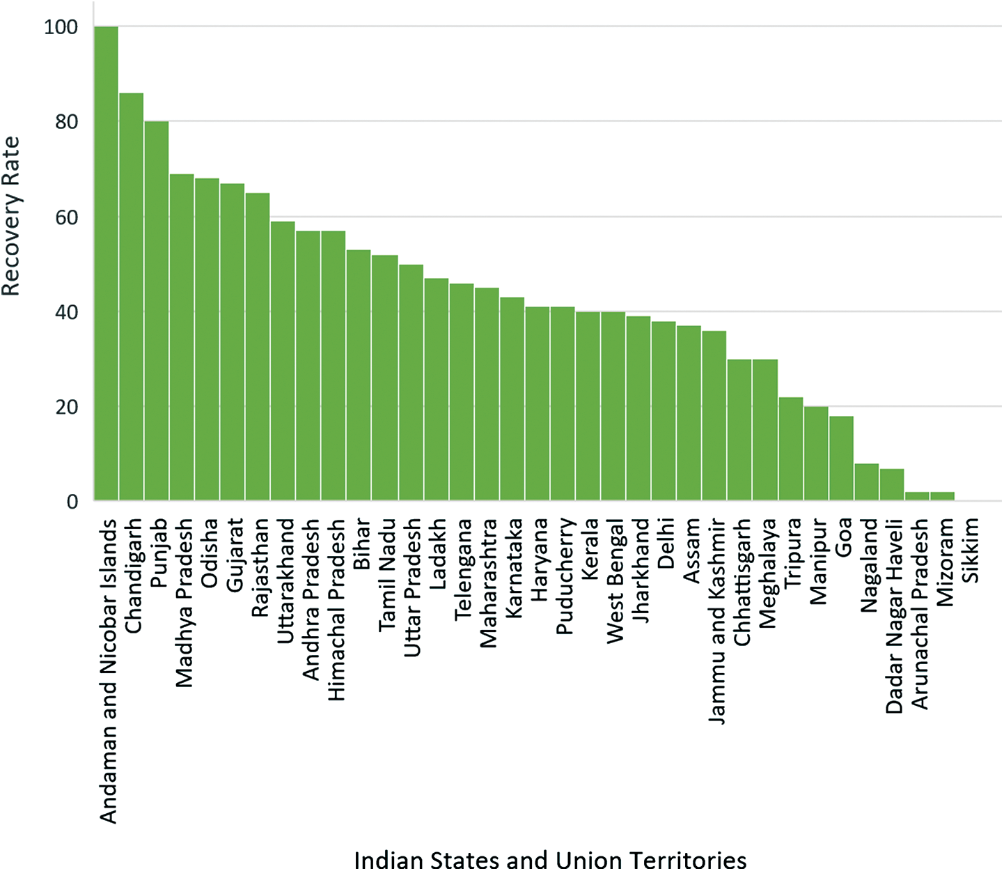
Figure 11: Recovery rate of Indian states and union territories

Fig. 12 shows the comparison between the mortality and the recovery rate of all the Indian states and Union territories.

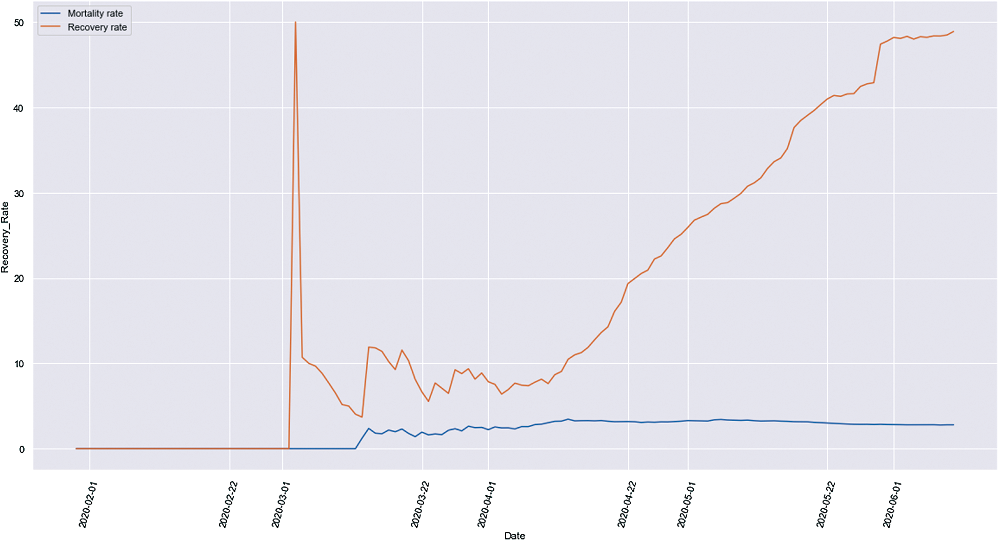
Figure 12: Mortality and recovery rate comparison

It is evident that initially, the mortality rate and the recovery rate were on the same level, and this was the situation in India till March 1, 2020. After this, we can see that the recovery rate started increasing at a very high rate while the mortality rate was still on a low. This increase in the recovery rate can be accounted for due to a higher testing rate and more awareness about the pandemic among people. Social distancing, the guidelines issued by the Government, and isolation helped in achieving such a high recovery rate in India. It is clearly shown that the recovery rate is increasing each day, and the mortality rate is tending more towards a constant value, which is a good sign for the country.

4.3 RMSE Evaluation

After the analysis of the total infected, discharges, and deaths due to COVID-19 in the states and Union Territories having more than 1000 cases in India, the performance of the trained regression model is evaluated using the root mean square error metrics. The RMSE metrics are calculated by validating the number of discharged patients and the number of deaths on further dates and calculation of corresponding error involved by using each regression algorithm. An RMSE value of 0.08 for PR, 0.66 for Decision Tree Regression, and 0.74 in case RF Regression for predicting discharged cases and an RMSE of 0.97, 0.15, and 0.14 respectively are obtained for the algorithms for prediction of death cases. Fig. 13 shows the RMSE values for all the three algorithms obtained for the discharges and death prediction.

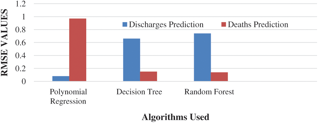
Figure 13: RMSE values for all the three algorithms obtained for the discharges and death prediction

4.3.1 Discharges Prediction

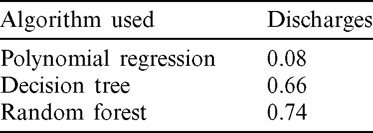
Machine learning approaches are valuable for prejudiced detection and cataloging tasks [41]. RMSE values of the three algorithms, namely Polynomial Regression, Decision Tree, and Random Forest, for the prediction of total discharges, are provided in Tab. 3. From Tab. 3, it is concluded that the Polynomial Regression model of degree 2 is the best suitable algorithm for predicting the number of discharge patients followed by Decision Tree and Random forest algorithms as an RMSE value of 0.08, shows the best performance in the prediction of the discharged patients. It shows that the curve of the cured or discharged patients having a quadratic growth in India, i.e., the number of discharges is increasing quadratically.

Table 3: RMSE values of regression algorithms for total discharges prediction

4.3.2 Deaths Prediction

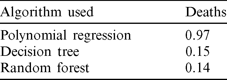
The RMSE values of the three algorithms, namely Polynomial Regression, Decision Tree, and Random Forest, for the prediction of total deaths, are provided in Tab. 4. Random Forest Algorithm shows a little bit better performance than the decision Tree for the validation set considered for this research as an RMSE value of 0.14 is obtained, which is far better than the values for the other two algorithms. For a wide variety of validation sets, it is concluded that the Random Forest and Decision Tree algorithms both hold good results in the prediction of deaths in various states and Union Territories in India. Polynomial regression shows the lowest accuracy among the three algorithms in the case of death prediction and hence not considered in building the final regression model.

Table 4: RMSE values of regression algorithms for total deaths prediction

5  Conclusion

This work seeks to carry out a comparative analysis of the prediction of an increase in the number of recovered and death cases in different states and union territories in India in the near future, as predicting these cases would help in estimating and arranging beds, ventilators, and other healthcare equipment’s on time and save many lives with proper facilities. The analysis includes the rising cases and deaths, mortality and recovery rates, gender and age-group based analysis, and case distribution. The research also focuses on developing the best regression model to predict the number of discharge patients and deaths in each state and union territory. In this work, the performance of the proposed framework is determined by using three machine learning regression algorithms, namely Polynomial Regression, Decision Tree Regression, and Random Forest Regression. The results show a comparative analysis of the states and union territories having more than 1000 cases, and the trained model is validated by testing it on further dates. The performance is evaluated using the RMSE metrics. The results show that Polynomial Regression with an RMSE value of 0.08 indicates the best performance in the discharged patients’ prognosis. In contrast, in the case of death prognosis, Random Forest, with an RMSE value of 0.14, shows a better performance than other techniques. Overall, this study helps make a detailed analysis and prediction and helps in understanding the entire scenario of COVID-19 across India.

Funding Statement: The author(s) received no specific funding for this study.

Conflicts of Interest: The authors declare that they have no conflicts of interest to report regarding the present study.

References

1.  N. Sharma, S. Acharya and S. Shukla. (2020). “Flattening the epidemic curve of corona outbreak: Beyond the realm of epidemiological mathematics,” EJPMR, vol. 7, no. 6, pp. 408–411.

2.  “India’s first coronavirus death confirmed in Karnataka,” The Economic Times, . [Online]. Available: https://economictimes.indiatimes.com/news/politics-and-nation/man-suspected-of-coronavirus-dies-after-returning-from-saudi arabia/articleshow/74574771.cms?utm_source=contentofinterest&utm_medium=text&utm_campaign=cppst.

3.  S. S. H. Kazmi, K. Hasan, S. Talib and S. Saxena. (2020). “COVID-19 and lockdown: A study on the impact on mental health,” . [Online]. Available: SSRN 3577515.

4.  R. Singh and P. K. Singh. (2020). “Connecting the dots of COVID-19 transmissions in India,” arXiv preprint arXiv:2004.07610.

5.  M. Naib. (2020). “At least 40,000 quarantined in India after a single priest spread coronavirus,” NBC News, . [Online]. Available: https://www.nbcnews.com/news/world/least-40-000-quarantined-india-after-single-priest-spread-coronavirus-n1171261.

6.  S. L. Badshah and A. Ullah. (2020). “Spread of coronavirus disease-19 among devotees during religious congregations,” Annals of Thoracic Medicine, vol. 15, no. 3, pp. 105.

7.  M. Chinazzi, J. T. Davis, M. Ajelli, C. Gioannini, M. Litvinova et al. (2020). , “The effect of travel restrictions on the spread of the 2019 novel coronavirus (COVID-19) outbreak,” Science, vol. 368, no. 6489, pp. 395–400.

8.  India Lockdown news, “India to be under complete lockdown for 21 days starting midnight: Narendra Modi.” [Online]. Available: https://economictimes.indiatimes.com/news/politics-and -nation/india-will-be-under-complete-lockdown-starting-midnight -narendra-modi/articleshow/74796908.cms?from=mdr.

This work is licensed under a Creative Commons Attribution 4.0 International License, which permits unrestricted use, distribution, and reproduction in any medium, provided the original work is properly cited.