DOI:10.32604/cmc.2021.013564
| Computers, Materials & Continua DOI:10.32604/cmc.2021.013564 | |
| Article |
Predicting the Electronic and Structural Properties of Two-Dimensional Materials Using Machine Learning
1Department of Physics, University of Tehran, Tehran, 14395-547, Iran
2Department of Mathematics and Physics, Leibniz Universität Hannover, Hannover, 30157, Germany
3Division of Computational Mechanics, Ton Duc Thang University, Ho Chi Minh City, Vietnam
4Faculty of Civil Engineering, Ton Duc Thang University, Ho Chi Minh City, Vietnam
*Corresponding Author: Timon Rabczuk. Email: timon.rabczuk@tdtu.edu.vn
Received: 30 August 2020; Accepted: 28 September 2020
Abstract: Machine-learning (ML) models are novel and robust tools to establish structure-to-property connection on the basis of computationally expensive ab-initio datasets. For advanced technologies, predicting novel materials and identifying their specification are critical issues. Two-dimensional (2D) materials are currently a rapidly growing class which show highly desirable properties for diverse advanced technologies. In this work, our objective is to search for desirable properties, such as the electronic band gap and total energy, among others, for which the accelerated prediction is highly appealing, prior to conducting accurate theoretical and experimental investigations. Among all available componential methods, gradient-boosted (GB) ML algorithms are known to provide highly accurate predictions and have shown great potential to predict material properties based on the importance of features. In this work, we applied the GB algorithm to a dataset of electronic and structural properties of 2D materials in order to predict the specification with high accuracy. Conducted statistical analysis of the selected features identifies design guidelines for the discovery of novel 2D materials with desired properties.
Keywords: 2D materials; machine-learning; gradient-boosted; band gap
Traditional methods for discovering new materials with desirable properties, such as the empirical trial and error methods using the existing structures and density functional theory (DFT) based method, have exceedingly high computational cost and typically require long research [1–4]. Machine learning methods can substantially reduce the computational costs and shorten the development cycle [5–7]. As an example, machine learning interatomic potentials (MLIPs) have been found as accurate alternatives for DFT computations with substantially lower computational cost [8,9]. MLIPs have been also proposed as alternatives for density functional perturbation theory simulations and for assessing the phononic and complex thermal properties [10–12]. Two-dimensional (2D) materials are currently among the fastest growing fields of research in material science and are extending across various scientific and engineering disciplines, owing to their fascinating electrical, optical, chemical, mechanical and thermal properties. 2D materials have attracted a lot of attention for applications such as nanosensors [5,13,14], magnon spintronics [15,16], molecular qubits [17,18], spin-liquid physics [19–21], energy storage/conversion systems [22–24] and catalytic application [25–28].
In the paradigm of materials informatics and accelerated materials discovery, the choice of feature set (i.e., attributes that capture aspect of lattice, chemistry and/or electronic structure) is critical [29,30]. Ideally, the feature sets should provide a simple physical basis for extracting major structural and chemical trends and enable rapid predictions of new material properties [31–34]. Machine learning has offered also novel ways to study the mechanical responses of various systems [35–37]. Here we show that machine learning methods can show superior ability in classification and prediction of properties of a rapidly extending class of materials, find the most important feature in classification and identifying the materials, thereby providing a feature selection approach for connecting among the components. In fact, in comparison with computational simulations, machine learning can identify patterns in large high-dimensional data sets effectively, extract useful information quickly [38] and discover hidden connections [38]. Typically, data processing consists of two sections: Data selection and feature engineering. The validity of data in both quality and quantity is a vital point in data selection. After data selection, one should extract suitable characteristics for the predicted target, which is called feature engineering. Feature engineering is the process of extracting features from raw data to enable the application of algorithms. In recent decades, the amount of scientific data collected approaches in the search for novel functional materials. In recent years, numerous extensive scientific data have been offered available in the form of online databases, for crystal structures [39,40] and materials properties [41–43]. In contrast to pure data-mining approaches, which focus on extracting knowledge from existing data [44], machine-learning approaches try to predict target properties directly [44], where a highly non-linear map between a crystal structure and its functional property of interest is approximated. In this context, machine learning offers an attractive framework for screening large collections of materials. In other words, developing an accurate machine learning model can substantially accelerate the identification of specific properties of materials, as the prediction of the property of interest for a given crystal structure bypasses computationally expensive ab-initio calculations.
In this work, our objective is to develop a machine learning model to predict important features of 2D-materials, including electronic band gap (Eg), work function (Ew), total energy (Et), unit-cell area (Aucell), fermi level (EFermi) and density of states (DOS), for which commonly employed DFT based approaches are computationally expensive. Since gradient-boosted (GB) algorithm provides highly accurate predictions both classification and regression, we used this tool in our exploration. We then consider a set of 2D materials and apply the developed methodology to identify the basic characteristic and relationship between different specifications.
Gradient boosted (GB) is an ensemble ML algorithm that uses multiple decision trees (DTs) as base learners [45]. Every DT is not independent, because a new added DT increases emphasis on the misclassified samples attained by previous DTs. It can be noticed that the residual of former DTs is taken as the input for the next DT. Then, the added DT is used to reduce residual, so that the loss decreases following the negative gradient direction in each iteration. Finally, the prediction result is determined based on the sum of results from all DTs. GB is a flexible non-parametric statistical learning technique for classification and regression. The GB method typically consists of three steps: feature selection [46,47], DT generation [48] and DT pruning [49]. Among them, the objective of feature selection is to retain features that exhibit sufficient classification performance and the objective of pruning is to make the tree simpler and thus more generalizable. Often features do not contribute equally to predict the target response. When interpreting a model, the first question usually is: what are those important features and how do they contributing in predicting the target response? A gradient boosted regression tree (GBRT) model derives this information from the fitted regression trees which intrinsically perform feature selection by choosing appropriate split points. Feature selection is the process of choosing a subset of features, from a set of original features, based on a specific selection criterion. The main advantages of feature selection are: (1) Reduction in the computational time of the algorithm, (2) Improvement in predictive performance, (3) Identification of relevant features, (4) Improved data quality and (5) Saving resources in subsequent phases of data collection. We can access this information via the instance attribute.
First, after collecting data we use the feature important algorithm for determining the valuable features with an impact on each other. In this regard, there are a few challenging aspects, such as heterogeneous features (different scales and distributions) and non-linear feature interactions. Furthermore, the data may contain some extreme values, such as the flat bands that appear in DOS with sharp peaks, therefore such a data set requires a robust regression technique [49]. In Fig. 1, the workflow for the present study is presented, which includes; collecting data properties, feature selection, classification and regression. For the classification process, the outcome of interest was binary with two categories: (i) Metal and (ii) Nonmetal. Dividing the materials to these two subsections is crucial for some computational and experimental approaches. For a binary outcome, a significant difference in the values of a continuous input variable for each outcome value shows that the variable can distinguish between the two outcome values. For the Gradient Boosting classification algorithm, the attribute feature importance ranks the importance of each feature for the constructed model. For each feature, the value of feature importance is between 0 and 1, where 0 means completely useless and 1 means perfect prediction. The sum of feature importance is always equal to 1. For analyzing the binary classification, we use The receiver operating characteristic (ROC) which is a measure of a classifier’s predictive quality that compares and visualizes the tradeoff between the model’s sensitivity and specificity. When plotted, a ROC curve displays true positive rate on the y-axis and the false positive rate on the x-axis on both a global average and a per-class basis. The ideal point is therefore the top-left corner of the plot, false positives are zero and true positives are one. This leads to another metric, area under the curve (AUC), which is a computation of the relationship between false positives and true positives. The higher the AUC, the better the model generally is. However, it is also important to inspect the steepness of the curve, as this describes the maximization of the true positive rate while minimizing the false positive rate. Besides, based on the optimal hyperparameters configuration, the regression models were constructed using different training set for each variable. Then, the test set was adopted to evaluate the performance of each model. The precision, recall and mean absolute error was utilized to analyze prediction results of each level and the accuracy values were used to assess the overall prediction performance. Based on the sensitivity analysis of indicators, the relative importance of each indicator was obtained.
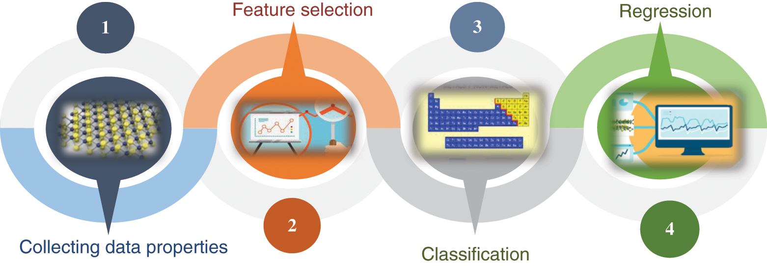
Figure 1: Workflow for the evaluation of 2D materials properties
In GB for gaining the high accuracy results, some parameters must be chosen so that they generally improve the performance of the algorithm by reducing overfitting [50]. These hyperparameters must be selected for the accurate optimization of results. Most of ML algorithms contain hyperparameters that need to be tuned. These hyperparameters should be adjusted based on the dataset rather than specifying manually. Generally, the hyperparameters search methods include grid search. The central challenge in machine learning is that we must perform well on new, previously unseen inputs, not just those on which our model was trained. The ability to perform well on previously unobserved inputs is called generalization. We require that the model learn from known examples and generalize from those known examples to new examples in the future. We use k-fold cross-validation only to estimate the ability of the model to generalize to new data. Tuning the hyperparameters is a very essential issue in GB predictions, because of the trivial overfitting problem. The general tuning strategy for exploring GB hyperparameters builds onto the basic and stochastic GB tuning strategies. There are different hyperparameters that we can tune and the parameters are different from base learner to base learner. We introduced some hyperparameters as usual in machine learning, because it is tedious to optimize them, especially knowing their correlation. In tree-based learners, which are the most common ones in GB applications, the following are the most commonly tuned hyperparameters. Learning-rate governs how quickly the model fits the residual error using additional base learners. If it is a smaller learning rate, it needs more boosting rounds and more time to achieve the same reduction in residual error, as one with a larger learning rate. In other words, it determines the contribution of each tree on the outcome and controls how quickly the algorithm proceeds down the gradient descent (learns) its values ranges from 0 to 1, with typical values between 0.001–0.3. Smaller values make the model robust to the specific characteristics of each tree, thus allowing to generalize better. Smaller values also facilitate to stop before overfitting, however, they increase the risk of not reaching the optimum with a fixed number of trees and are therefore more computationally demanding, noting that this hyperparameter is also called shrinkage. The most important regularization technique for GB is shrinkage, the idea is basically to conduct slow learning by shrinking the predictions of each tree by smaller learning-rate, helpful to achieve re-enforce concepts. A lower learning-rate requires a higher number of estimators to get to the same level of training error. Generally, the smaller this value, the more accurate the model can be developed, but it also requires more trees in the sequence. The two other hyperparameters, the subsample and the number of estimators are regularization hyperparameters. Subsampling is the fraction of the total training set that can be used in any boosting round. A low value may lead to under-fitting issues. In contrary, a very high value can lead to over-fitting issue. Besides regularization, increasing the number of training examples and reducing the number of input and features, are more advantages for fixing overfitting. The depth of the individual trees is one aspect of model complexity. The depth of the trees controls the degree of feature interactions that our model can fit. For example, if one wants to capture the interaction between a feature latitude and a feature longitude our trees need a depth of at least two to capture this. Unfortunately, the degree of feature interactions is not known in advance but it is usually fine to assume that it is fairly low in practice, a depth of 4–6 usually gives the best results. In scikit-learn [51], we can constrain the depth of the trees using the maximum depth argument. Despite interpolating these parameters two more common overfitting and underfitting problems for the GB algorithm addressed the unfavorable results. We can address underfitting by increasing the capacity of the model. Capacity refers to the ability of a model to fit a variety of functions, more capacity means that a model can fit more types of functions for mapping inputs to outputs. Increasing the capacity of a model is easily achieved by changing the structure of the model, such as adding more layers and/or more nodes to layers. Because an under-fit model is so easily addressed, it is more common to have an over-fit model. Both train-test splits and k-fold cross-validation are examples of resampling methods, although both of these methods cannot overcome the overfitting, they can reduce these complications, but the regularization is one of the best methods for the resistance of data for overfitting. An over-fit model is easily diagnosed by monitoring the performance of the model during training by evaluating it on both a training dataset and on a holdout validation dataset. To get highly accurate predictions, we employed the iteration process for optimizing hyperparameters: first, we choose loss based on our problem at hand (i.e., target metric), then pick number of estimators as large as (computationally) possible (e.g., 3000). Next, we tune the maximum depth, learning-rate, subsample and maximum features via iteration process in a loop that we can achieve to less difference between the training and test deviance (find the Apendix). All other parameters were left to their default values.
The considered dataset of 2D-materials considered in this work includes more than 1,500 compounds, taken from the recent work of Haastrup et al. [50]. In the aforementioned work, authors calculated structural, thermodynamic, elastic, electronic, magnetic and optical properties of an extensive ensemble of 2D-materials by state-of-the-art DFT within the many-body perturbation theory. In this paper, we model the structure-property relationship via machine learning for 2D materials. Among these data, we select thermodynamically and dynamically stable compounds. Worthy to note that dynamically stable lattices do not show imaginary frequencies in the phonon dispersions. With considered stabilities criteria, 981 compounds were selected. In these types of datasets, the materials vary from a range of nonmetal up to metal that these sorts kinds of materials are applicable in many research areas. The kind of crystal structure distributed over more than 50 different structures, also the unit cell and internal coordinates of the atoms are relaxed in both a spin-paired (NM), ferromagnetic (FM) and anti-ferromagnetic (AFM) configuration. The projected density of states (PDOS) is another label that is a useful tool for identifying which atomic orbitals comprise a band. The electron density is determined self-consistently on a uniform k-point grid of density 12.0/Å. From this density, the PBE band structure is computed non-self consistently at 400 K-points distributed along the band path. Also, The fermi level is calculated using the PBE xc-functional including spin-orbit coupling (SOC) for all metallic compounds in the database. For metallic compounds, the work function is obtained as the difference between the Fermi energy and the asymptotic value of the electrostatic potential in the vacuum region. Electronic polarizability, Plasma frequencies and speed of sound are other labels that we consider for the prediction of our targets. Fig. 2a shows histograms for some of the features and the response. We can see that they are quite different. The band gap and density of states are left-skewed, the area of the unit cell is bi-modal and the total energy is right-skewed. As shown in Fig. 2a the total energy varies a range from 100 ev to 0 and the work function ranged from 2.5–7.5 ev that describes the non-equal distribution of datasets. For showing the relationship between these features, Correlation is a well-known similarity measure between two features. If two features are linearly dependent, then their correlation coefficient is  1. If the features are uncorrelated, the correlation coefficient is 0. The association between the features is found out by using the correlation method. Because the GB algorithm is not capable in calculating the important score of two attributes in datasets, the pearson’s correlation method is used for finding the association between the continuous features and the class feature. According to Fig. 2b, the correlation between the datasets is shown, that for each pair of features x and y, the square of the correlation coefficient
  were calculated and the intensity of color show the intensity of correlation.
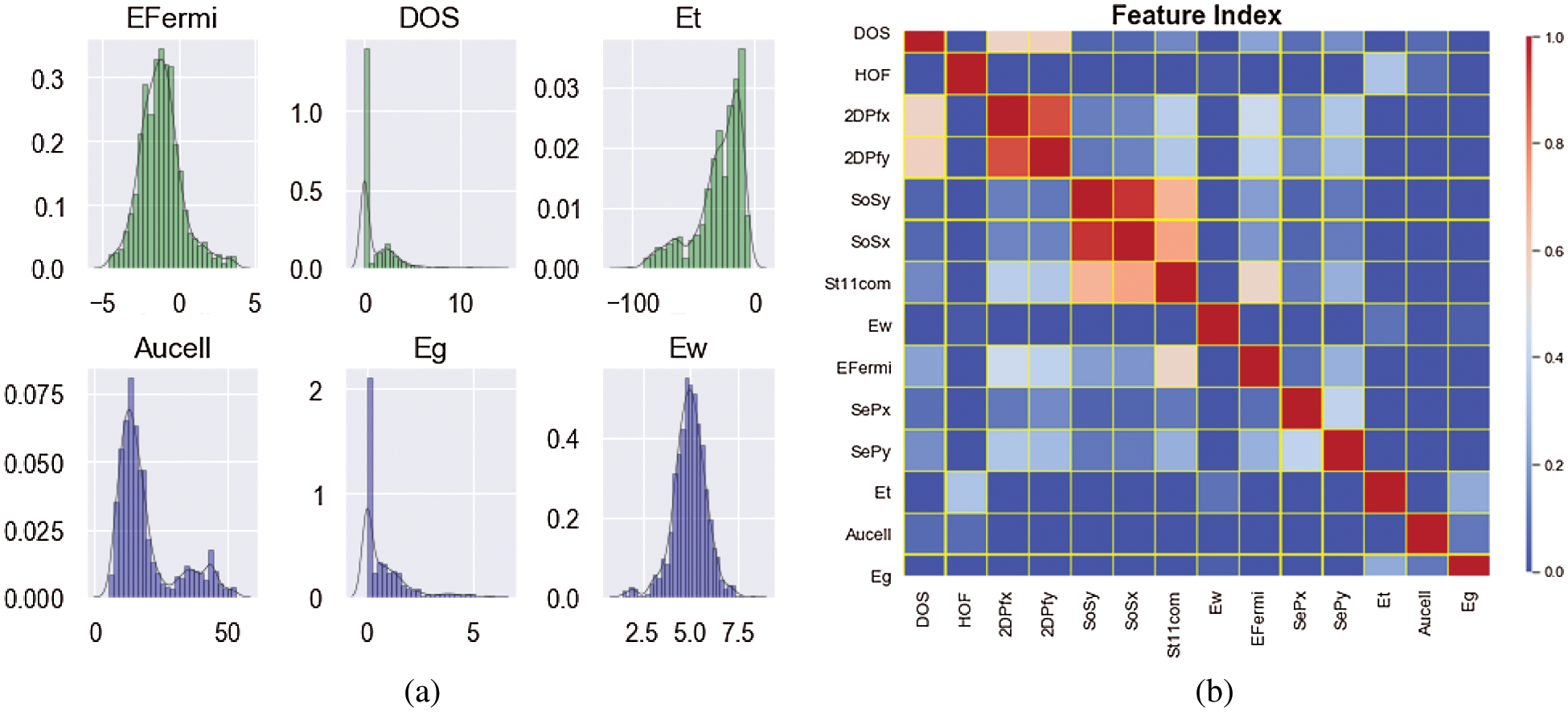
Figure 2: (a) The distribution of components and (b) a heat map of the pearson correlation coefficient matrix for the 14 features
For a prediction of the classification based on machine learning, we discuss the gradient boosting model, considering 15 features for predicting targets. The total of 15 features includes the following: The heat of formation (HOF), band gap (Eg), density of states at the fermi energy (DOS), total energy (Et), fermi level (EFermi), speed of sound (x) (SoSx), speed of sound (y) (SoSy), work function (Ew), static electronic polarizability (x) (SePx), static electronic polarizability (y) (SePy), direct band gap (DirEg), stiffness tensor, 11-component (St11com), 2D plasma frequency (x) (2DPfx), 2D plasma frequency (y) (2DPfy), area of unit-cell (AUcell). Because among these features some attributes such as the density of states, two-dimension plasma frequency in x and y direction, the direct band gap and band gap have a direct impact on classification on materials in two such groups so we neglect these categories although with attention to these features the effect of other features decreases. With 10-fold cross-validation train the models using 90% materials (training set) and evaluate their performance using mean absolute error (MAE) for the remaining 10% materials (test set). we focus on loss functions such as MAE, which is less sensitive to outliers and also to be able to apply the method to a classification problem with a loss function such as deviance, or log loss. For the feature engineering process, we consider 10 important features that the importance of each feature shown in Fig. 3a. A novel candidate material is first classified as a metal or a nonmetal. If the material is classified as a nonmetal, Eg is predicted, here as classification as a metal implies that the material has no Eg (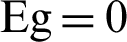 ). The accuracy of the metal/nonmetal classifier is reported as the AUC of the ROC plot (Fig. 3b). Acquired ROC curve illustrates the model’s ability to differentiate between metallic and nonmetallic input two-dimension materials. It plots the prediction rate for nonmetal (correctly vs. incorrectly predicted) throughout the full spectrum of possible prediction thresholds. An area of 1.0 represents a perfect test, whereas an area of 0.5 characterizes a random guess (the dashed line). The model shows excellent external predictive power with the area under the curve at 0.98, a nonmetal-prediction success rate (sensitivity) of 0.98, a metal-prediction success rate (specificity) of 0.98 and an overall classification accuracy (R-squared) of 0.93 (Fig. 3a). For the complete set of 980 2D lattice, this corresponds to about 20 misclassified materials, including 10 misclassified metals and 10 misclassified nonmetals.
Figure 3: (a) Feature importance for GB classification of metal and nonmetal (b) ROC curve of metal/nonmetal classification
The model exhibits a positive bias toward predicting metals, where bias refers to whether the ML model tends to over- or under-estimate the predicted property. This low false-metal rate is acceptable as the model is unlikely to misclassify a novel and potentially interesting nonmetal as a metal. Overall, the metal classification model is robust enough to handle the full complexity of the periodic table. The direction has about 50% direct impact on classification in contrast to the other features. For the regression process, the visualization result of feature importance in this paper is shown in Figs. 4a–4f, which displays the relative importance of the 14 most influential predictor variables for each target.
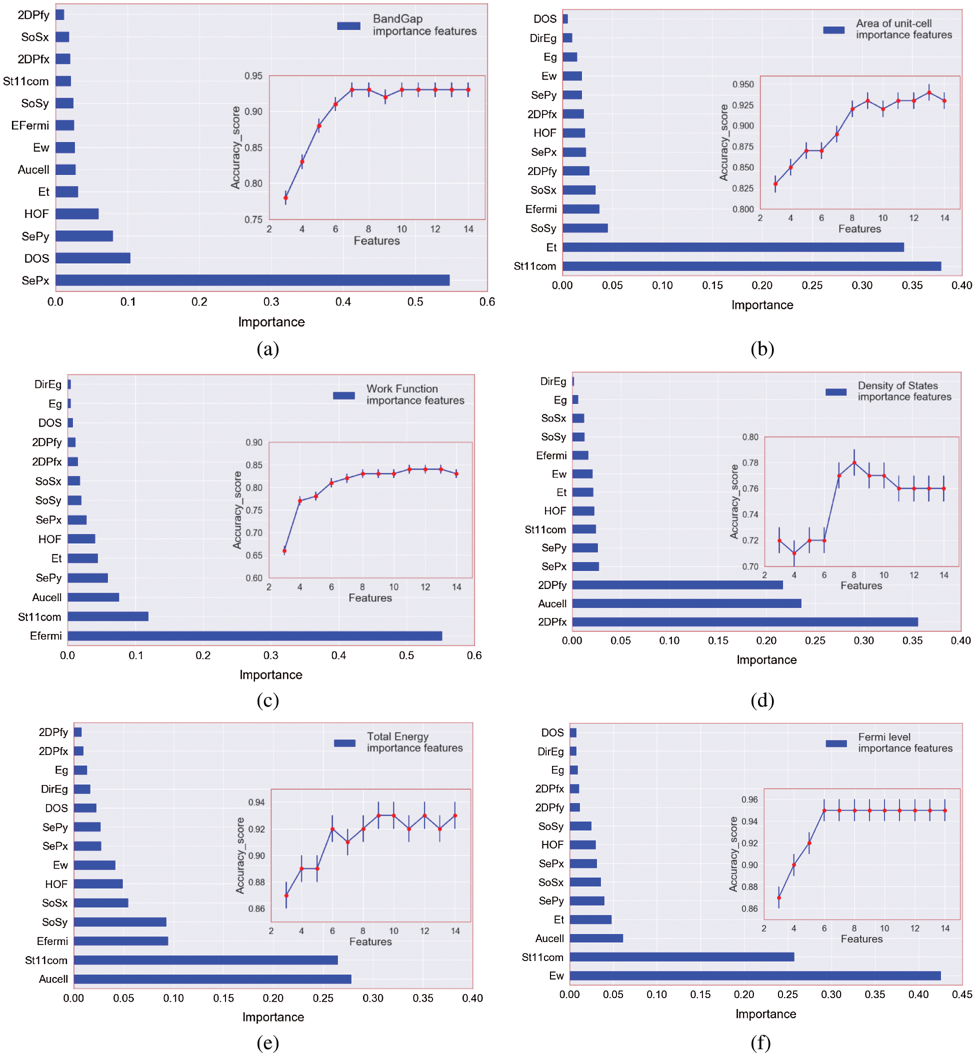
Figure 4: (a–f) Feature importance of each category and accuracy_score variation as the feature number increase
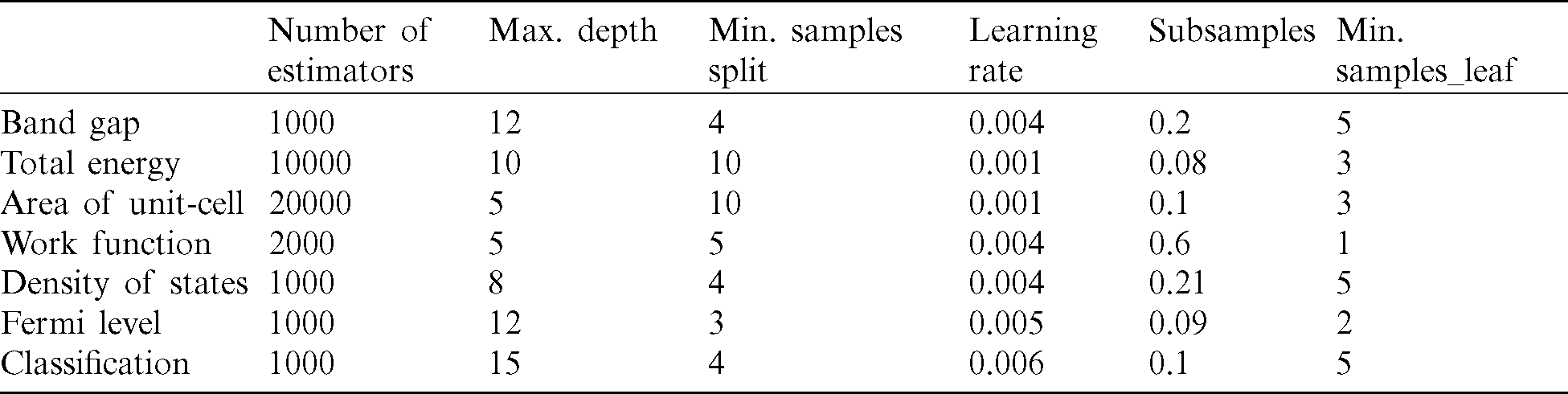
Since these measures are relative, a value of 1 was assigned to the most important predictor and the others were scaled accordingly. There is a clear differential effect between the models. For instance, for band gap target, static electron polarization x and density of states have more percent in feature values relate to other variables but in contrast, these two variables are far less important in the total energy model. The work function is the most relevant predictor in the fermi level model, while it is far less important in the area of the unit cell model. Among the other influential predictors in the area of the unit cell, stiffness tensor and total energy are more important features for identifying the target. For the density of state, we find the presence of an area of the unit cell, two-dimension plasma frequency in x and y-direction. For the work function, the fermi level is the most influential predictor, followed by the stiffness tensor and the area of the unit cell. Figs. 4a–4f show how the feature in the prediction of the targets changes under the process of extracting key-features. Remarkably, we found that accuracy-score increases almost monotonically in all cases, which indicates that a feature with a higher feature score has stronger predictive power. Through this process, we selected the most important features for each target property. For Eg, the score abruptly increases when the number of features is larger than five (Fig. 4a). This means that at least five features are required to predict band gap within MAE of 0.16 eV. In the case of DOS, seven features comprise a minimal set to predict the density of states within an MAE of 0.53 eV (Fig. 4d). Tab. 1 showed the minimum selected features for the best result in both MSE and accuracy scores. Key-features extracted from the feature importance score of the GBRT method can have various implications for a fast search for new material. For instance, selected key-features can be utilized as an optimal set of features in another type of ML algorithms such as classification. With a smaller number of features, as seen in Fig. 4 the prediction accuracy is lower than that with all features. However, it is notable that regression with the top key-features selected for targets provides a good approximation to that with the full features. The results of the variables regression model are plotted in Fig. 5. Fig. 5a presents the prediction of Eg, that the results show that the MAE of test sets for Eg is 0.16 eV. Even though the number of the current dataset was limited, it is noteworthy that the accuracy of the predictive model of Eg, Et, Aucell, Efermi. Besides, a statistical profile of these predictions, along with that of the six other regression models, is provided in Tab. 1, which includes metrics such as the MAE and coefficient of determination (R2). Similar to the classification model, the GBRT model exhibits a positive predictive bias. The biggest errors in DOS, come from materials with narrow band gaps, that is, the scatter in the lower-left corner in Fig. 5c. similar results for the other five targets is shown the power of the prediction but in the density of the state and work function the less accuracy among the variables exists. The outcome of the interpolating of parameters was shown in Tab. 2. The result can be slightly improved by decreasing the learning rate and adjusting subsample related to it. With attention to these hyperparameters, the performance measure reported by 10-fold cross-validation is then the average of the values computed in the loop. This approach can be computationally expensive but does not waste too much data (as is the case when fixing an arbitrary validation set), which is a major advantage in problems such as inverse inference where the number of samples is very small.
Table 1: The best performance of the model after feature selection
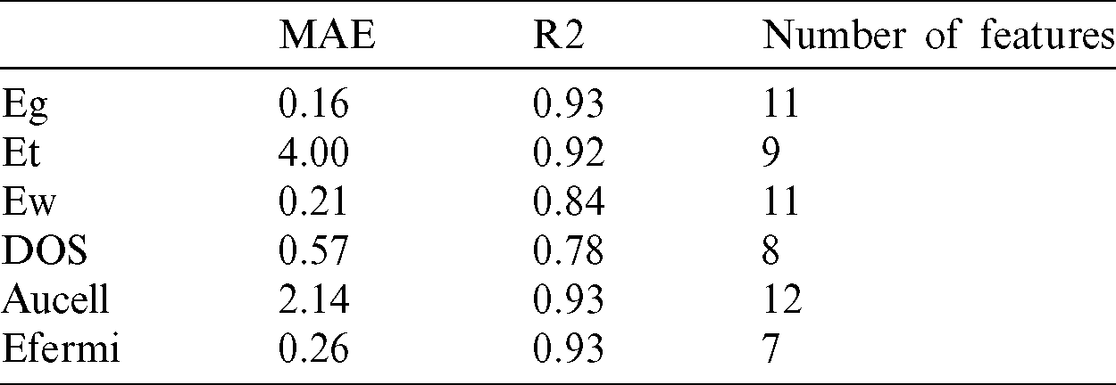
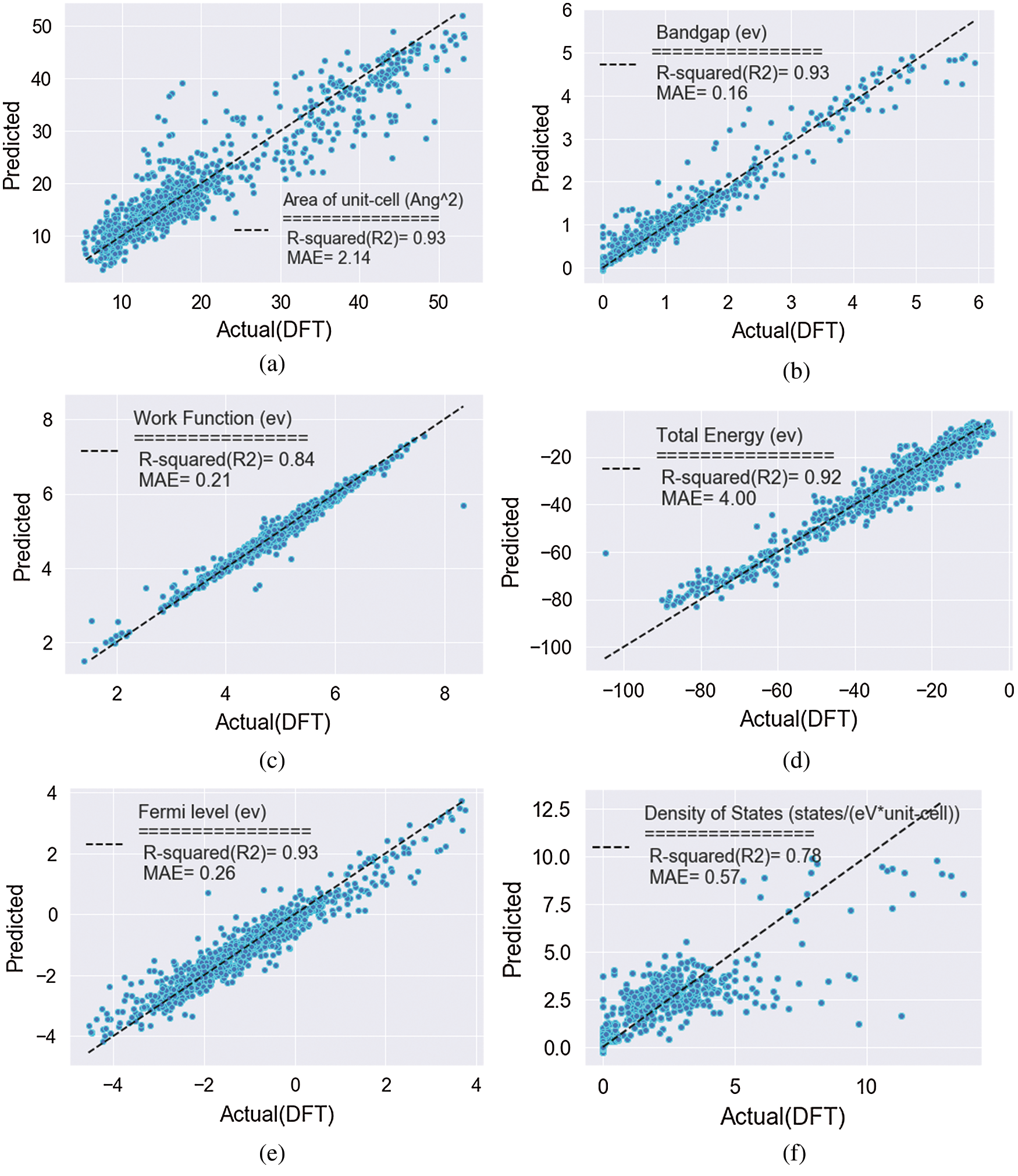
Figure 5: (a–f) Predicted vs. calculated values for the regression GB models: (a) band gap (Eg), (b) area of unit-cell (Aucell), (c) density of states (DOS), (d) work function (Ew), (e) fermi level (Efermi) and (f) total energy (Et)
Table 2: Summarizes the best performance of the model after feature selection. In the last line of the table, the hyperparameters of classification of metal and nonmetal were shown
In comparison, we plot the residual gradient. boosting regression with train test split that the accuracy of the train and test data, showing not any different and the R2-squared are similar to the 10-fold validation.
In this work, we show that machine learning can be effectively employed to rapidly characterize the specification and predict the intrinsic properties of 2D materials. In particular, it is confirmed that the use of feature engineering in the machine learning models enhances the accuracy, computational cost and prediction power. However, we note that an explicit relationship between features and properties is still difficult to obtain directly from the feature importance score and additional steps are required. The models developed in this work are capable of predicting electrical and structural properties for diverse 2D lattices with accuracies compatible with DFT methods. This is in fact a promising finding for the use in high-throughput material screening and could be valuable in influencing engineering decisions and bring a new dynamic to materials discovery.
Acknowledgement: E. A. acknowledges the University of Tehran Research Council for support of this study.
Funding Statement: The authors received no specific funding for this study.
Conflicts of Interest: The authors declare that they have no conflicts of interest to report regarding the present study.
References
1. X. Wang, J. Zhuang, Q. Peng and Y. Li. (2005). “A general strategy for nanocrystal synthesis,” Nature, vol. 467, pp. 121–124.
2. A. R. Oganov, C. J. Pickard, Q. Zhu and R. J. Needs. (2019). “Structure prediction drives materials discovery,” Nature Reviews Materials, vol. 4, no. 5, pp. 331–348.
3. A. R. Oganov, A. O. Lyakhov and M. Valle. (2011). “How evolutionary crystal structure prediction works-and why,” Accounts of Chemical Researches, vol. 44, no. 3, pp. 227–237.
4. H. Koinuma and I. Takeuchi. (2004). “Combinatorial solid-state chemistry of inorganic materials,” Nature Materials, vol. 3, pp. 429–438.
5. H. Sahu, W. Rao, A. Troisi and H. Ma. (2018). “Toward predicting efficiency of organic solar cells via machine learning and improved descriptors,” Advanced Energy Materials, vol. 8, no. 24, 1801032.
6. J. P. Correa-Baena, K. Hippalgaonkar, J. Van Duren, S. Jaffer, V. R. Chandrasekhar et al. (2018). , “Accelerating materials development via automation, machine learning, and high-performance computing,” Joule, vol. 2, no. 8, pp. 1410–1420.
7. G. H. Gu, J. Noh, I. Kim and Y. Jung. (2019). “Machine learning for renewable energy materials,” Journal of Materials Chemistry A, vol. 7, no. 29, pp. 17096–17117.
8. E. V. Podryabinkin, E. V. Tikhonov, A. V. Shapeev and A. R. Oganov. (2019). “Accelerating crystal structure prediction by machine-learning interatomic potentials with active learning,” Physical Review B, vol. 99, pp. 064114.
9. K. Gubaev, E. V. Podryabinkin, G. L. W. Hart and A. V. Shapeev. (2019). “Accelerating high-throughput searches for new alloys with active learning of interatomic potentials,” Computational Materials Science, vol. 156, pp. 148–156.
10. B. Mortazavi, E. V. Podryabinkin, S. Roche, T. Rabczuk, X. Zhuang et al. (2020). , “Machine-learning interatomic potentials enable first-principles multiscale modeling of lattice thermal conductivity in graphene/borophene heterostructures,” Materials Horizons, vol. 7, no. 9, pp. 2359–2367. [Google Scholar]
11. V. V. Ladygin, P. Y. Korotaev, A. V. Yanilkin and A. V. Shapeev. (2020). “Lattice dynamics simulation using machine learning interatomic potentials,” Computational Materials Science, vol. 172, 109333. [Google Scholar]
12. P. Korotaev, I. Novoselov, A. Yanilkin and A. Shapeev. (2019). “Accessing thermal conductivity of complex compounds by machine learning interatomic potentials,” Physical Review B, vol. 100, no. 14, pp. 144308. [Google Scholar]
13. O. Lopez-Sanchez, D. Lembke, M. Kayci, A. Radenovic and A. Kis. (2013). “Ultrasensitive photodetectors based on monolayer MoS2,” Nature Nanotechnoogy, vol. 8, no. 7, pp. 497–501. [Google Scholar]
14. T. O. Wehling. (2008). “Molecular doping of graphene,” Nano Letters, vol. 8, no. 1, pp. 173–177. [Google Scholar]
15. W. Xing, L. Qiu, X. Wang, Y. Yao, Y. Ma et al. (2019). , “Magnon transport in quasi-two-dimensional van der waals antiferromagnets,” Physical Review, vol. 9, no. 1, pp. 11026. [Google Scholar]
16. S. Tacchi, P. Gruszecki, M. Madami, G. Carlotti, J. W. Klos et al. (2015). , “Universal dependence of the spin wave band structure on the geometrical characteristics of two-dimensional magnonic crystals,” Scientifics Reports, vol. 5, no. 1, pp. 10367. [Google Scholar]
17. M. Ye, H. Seo and G. Galli. (2019). “Spin coherence in two-dimensional materials,” Npj Computational Materials, vol. 5, no. 1, pp. 44. [Google Scholar]
18. E. Coronado. (2020). “Molecular magnetism: From chemical design to spin control in molecules, materials and devices,” Nature Review Materials, vol. 5, no. 2, pp. 87–104. [Google Scholar]
19. M. Yamashita, N. Nakata, Y. Senshu, M. Nagata, H. M. Yamamoto et al. (2010). , “Highly mobile gapless excitations in a two-dimensional candidate quantum spin liquid,” Science, vol. 328, no. 5983, pp. 1246–1248. [Google Scholar]
20. S. Wessel, B. Normand, M. Sigrist and S. Haas. (2001). “Order by disorder from nonmagnetic impurities in a two-dimensional quantum spin liquid,” Physical Review Letters, vol. 86, no. 6, pp. 1086–1089. [Google Scholar]
21. Z. Y. Meng, T. C. Lang, S. Wessel, F. F. Assaad and A. Muramatsu. (2010). “Quantum spin liquid emerging in two-dimensional correlated Dirac fermions,” Nature, vol. 464, no. 7290, pp. 847–851. [Google Scholar]
22. M. Mousavi, A. Habibi-Yangjeh and S. R. Pouran. (2018). “Review on magnetically separable graphitic carbon nitride-based nanocomposites as promising visible-light-driven photocatalysts,” Journal of Materials Science: Materials in Electronics, vol. 29, no. 3, pp. 1719–1747. [Google Scholar]
23. Y. Liu and X. Peng. (2017). “Recent advances of supercapacitors based on two-dimensional materials,” Applied Materials Today, vol. 7, pp. 1–12. [Google Scholar]
24. J. B. Goodenough and Y. Kim. (2010). “Challenges for rechargeable Li batteries,” Chemistry of Materials, vol. 22, no. 3, pp. 587–603. [Google Scholar]
25. A. Alarawi, V. Ramalingam and J. H. He. (2019). “Recent advances in emerging single atom confined two-dimensional materials for water splitting applications,” Materials Today Energy, vol. 11, pp. 1–23. [Google Scholar]
26. J. Liu, H. Wang and M. Antonietti. (2016). “Graphitic carbon nitride ‘reloaded’: Emerging applications beyond (photo)catalysis,” Chemical Society Reviews, vol. 45, no. 8, pp. 2308–2326. [Google Scholar]
27. Q. Wang, B. Jiang, B. Li and Y. Yan. (2016). “A critical review of thermal management models and solutions of lithium-ion batteries for the development of pure electric vehicles,” Renewable and Sustainable Energy Reviews, vol. 64, pp. 106–128. [Google Scholar]
28. P. Kumar, E. Vahidzadeh, U. K. Thakur, P. Kar, K. M. Alam et al. (2019). , “C3N5: A low bandgap semiconductor containing an azo-linked carbon nitride framework for photocatalytic, photovoltaic and adsorbent applications,” Journal of the American Chemical Society, vol. 141, no. 13, pp. 5415–5436. [Google Scholar]
29. B. Kailkhura, B. Gallagher, S. Kim, A. Hiszpanski and T. Y. J. Han. (2019). “Reliable and explainable machine-learning methods for accelerated material discovery,” Npj Computational Materials, vol. 5, no. 1, pp. 108. [Google Scholar]
30. S. Lu, Q. Zhou, L. Ma, Y. Guo and J. Wang. (2019). “Rapid discovery of ferroelectric photovoltaic perovskites and material descriptors via machine learning,” Small Methods, vol. 3, no. 11, 1900360. [Google Scholar]
31. G. Pilania, A. Mannodi-Kanakkithodi, B. P. Uberuaga, R. Ramprasad, J. E. Gubernatis et al. (2016). , “Machine learning bandgaps of double perovskites,” Scientific Reports, vol. 6, no. 1, pp. 19375. [Google Scholar]
32. G. Pilania, C. Wang, X. Jiang, S. Rajasekaran and R. Ramprasad. (2013). “Accelerating materials property predictions using machine learning,” Scientific Reports, vol. 3, no. 1, pp. 2810. [Google Scholar]
33. M. Rupp, A. Tkatchenko, K. R. Müller and O. A. Von Lilienfeld. (2012). “Fast and accurate modeling of molecular atomization energies with machine learning,” Physical Review Letters, vol. 108, no. 5, pp. 58301. [Google Scholar]
34. S. Lu, Q. Zhou, Y. Ouyang, Y. Guo, Q. Li et al. (2018). , “Accelerated discovery of stable lead-free hybrid organic-inorganic perovskites via machine learning,” Nature Communications, vol. 9, no. 1, pp. 3405. [Google Scholar]
35. B. Mortazavi, E. V. Podryabinkin, I. S. Nvikov, S. Roche, T. Rabczuk et al. (2020). , “Efficient machine-learning based interatomic potentials for exploring thermal conductivity in two-dimensional materials,” Journal of Physics: Materials, vol. 3, 02LT02. [Google Scholar]
36. H. Mortazavi. (2018). “Designing a multidimensional pain assessment tool for critically Ill elderly patients: An agenda for future research,” Indian Journal of Critical Care Medicine, vol. 22, no. 5, pp. 390–391. [Google Scholar]
37. H. Mortazavi. (2018). “Could art therapy reduce the death anxiety of patients with advanced cancer? An interesting question that deserves to be investigated,” Indian Journal of Palliative Care, vol. 24, no. 3, pp. 387–388. [Google Scholar]
38. M. H. S. Segler and M. P. Waller. (2017). “Neural-symbolic machine learning for retrosynthesis and reaction Prediction,” Chemistry A European Journal, vol. 23, no. 25, pp. 5966–5971. [Google Scholar]
39. T. Yamashita, N. Sato, H. Kino, T. Miyake, K. Tsuda et al. (2018). , “Crystal structure prediction accelerated by Bayesian optimization,” Physical Review Materials, vol. 2, no. 1, 13803. [Google Scholar]
40. C. C. Fischer, K. J. Tibbetts, D. Morgan and G. Ceder. (2006). “Predicting crystal structure by merging data mining with quantum mechanics,” Nature Materials, vol. 5, no. 8, pp. 641–646. [Google Scholar]
41. S. Curtarolo, W. Setyawan, G. L. W. Hart, M. Jahnatek, R. V. Chepulskii et al. (2012). , “AFLOW: An automatic framework for high-throughput materials discovery,” Computational Materials Science, vol. 58, pp. 218–226. [Google Scholar]
42. C. Draxl and M. Scheffler. (2018). “NOMAD: The FAIR concept for big data-driven materials science,” MRS Bulletin, vol. 43, no. 9, pp. 676–682. [Google Scholar]
43. J. E. Saal, S. Kirklin, M. Aykol, B. Meredig and C. Wolverton. (2013). “Materials design and discovery with high-throughput density functional theory,” JOM, vol. 65, no. 11, pp. 1501–1509. [Google Scholar]
44. N. Huber, S. R. Kalidindi, B. Klusemann and C. J. Cyron. (2020). “Editorial: Machine learning and data mining in materials science,” Frontiers of Materials, vol. 7, pp. 51. [Google Scholar]
45. N. Claussen, B. A. Bernevig and N. Regnault. (2020). “Detection of topological materials with machine learning,” Physical Review B, vol. 101, no. 24, 245117. [Google Scholar]
46. Danishuddin and A. U. Khan. (2016). “Descriptors and their selection methods in QSAR analysis: Paradigm for drug design,” Drug Discovery Today, vol. 21, no. 8, pp. 1291–1302. [Google Scholar]
47. I. Ponzoni, V. Sebastián-Pérez, C. Requena-Triguero, C. Roca, M. J. Martínez et al. (2017). , “Hybridizing feature selection and feature learning approaches in QSAR modeling for drug discovery,” Scientific Reports, vol. 7, no. 1, pp. 2403. [Google Scholar]
48. Z. Jagga and D. Gupta. (2015). “Machine learning for biomarker identification in cancer research–-Developments toward its clinical application,” Personalized Medicine, vol. 12, no. 4, pp. 371–387. [Google Scholar]
49. F. Esposito, D. Malerba, G. Semeraro and J. Kay. (1997). “A comparative analysis of methods for pruning decision trees,” IEEE Transactions on Pattern Analysis and Machine Intelligence, vol. 19, no. 5, pp. 476–491. [Google Scholar]
50. S. Haastrup, M. Strange, M. Pandey, T. Deilmann, P. S. Schmidt et al. (2018). , “The computational 2D materials database: High-throughput modeling and discovery of atomically thin crystals,” 2D Materials, vol. 5, no. 4, pp. 42002. [Google Scholar]
51. F. F. Pedregosa, G. Varoquaux, A. Gramfort, V. Michel, B. Thirion et al. (2011). , “Scikit-learn: Machine learning in python,” Journal of Machine Learning Research, vol. 12, pp. 2825–2830. [Google Scholar]
 | This work is licensed under a Creative Commons Attribution 4.0 International License, which permits unrestricted use, distribution, and reproduction in any medium, provided the original work is properly cited. |