DOI:10.32604/cmc.2021.014526
| Computers, Materials & Continua DOI:10.32604/cmc.2021.014526 | |
| Article |
Street-Level IP Geolocation Algorithm Based on Landmarks Clustering
1PLA Strategic Support Force Information Engineering University, Zhengzhou, 450001, China
2State Key Laboratory of Mathematical Engineering and Advanced Computing, Zhengzhou, 450001, China
3Cyberspace Security Key Laboratory of Sichuan Province, Chengdu, 610000, China
4China Electronic Technology Cyber Security Co., Ltd., Chengdu, 610000, China
5University of Goettingen, Goettingen, 37075, Germany
*Corresponding Author: Fenlin Liu. Email: liufenlin@vip.sina.com
Received: 26 September 2020; Accepted: 27 October 2020
Abstract: Existing IP geolocation algorithms based on delay similarity often rely on the principle that geographically adjacent IPs have similar delays. However, this principle is often invalid in real Internet environment, which leads to unreliable geolocation results. To improve the accuracy and reliability of locating IP in real Internet, a street-level IP geolocation algorithm based on landmarks clustering is proposed. Firstly, we use the probes to measure the known landmarks to obtain their delay vectors, and cluster landmarks using them. Secondly, the landmarks are clustered again by their latitude and longitude, and the intersection of these two clustering results is taken to form training sets. Thirdly, we train multiple neural networks to get the mapping relationship between delay and location in each training set. Finally, we determine one of the neural networks for the target by the delay similarity and relative hop counts, and then geolocate the target by this network. As it brings together the delay and geographical coordinates clustering, the proposed algorithm largely improves the inconsistency between them and enhances the mapping relationship between them. We evaluate the algorithm by a series of experiments in Hong Kong, Shanghai, Zhengzhou and New York. The experimental results show that the proposed algorithm achieves street-level IP geolocation, and comparing with existing typical street-level geolocation algorithms, the proposed algorithm improves the geolocation reliability significantly.
Keywords: IP geolocation; neural network; landmarks clustering; delay similarity; relative hop
IP geolocation technology aims to obtain the geographic location of a given IP address [1]. It has been widely used in advertisement delivery, user positioning, tracking attack source and so on [2–4]. High-precision and reliable IP geolocation technology is getting more and more attention in the development of the Internet [5]. But geolocating a host with its IP address is still a challenging problem because there is no direct relationship between geographic location and IP address [6]. Therefore, the research on IP geolocation technology is of great practical significance.
The existing methods of IP geolocation mainly include the geolocation method based on IP location databases and the method based on network measurement.
The method based on IP location databases mainly determines the location of an IP through query, and the databases used mainly include Whois [7], IP2Location [8] and Maxmind [9]. However, the accuracy of such databases can only reach the national-level, and it is difficult for them to be used for more accurate geolocation [10,11]; moreover, geolocation results may be unreliable due to belated database update.
The IP geolocation methods based on network measurement mainly estimate the geographical location of a target IP by using the delay, topology and other information obtained through the network measurement on the target IP. These methods can be divided into city-level IP geolocation methods and street-level IP geolocation methods.
City-level IP geolocation methods include GeoPing [6], CBG (Constraint-Based Geolocation) [12], Octant [13], GeoWeight [14], LBG (Learning-based Geolocation) [15], Point of Presence (PoP) Analysis based Geolocation [16], GBLC (Landmark Clustering based Geolocation) [17], PoP Partition based Geolocation [18], Geo-PoP [19]. These methods mainly use attributes such as delay, hop count and network structure to constrain the geographical location of the target IP to a certain area or use the landmark of the known geographical location as its estimated location. Among them, GeoPing takes the location of the landmark whose delay vector resembles the target most closely as the location of the target; CBG calculates the “delay-distance” conversion coefficient of each probes, and estimates the location of the target IP through multiple probes; Octant and GeoWeight improve the CBG, on the basis of calculating the relationship between delay and distance, they constrain the location of targets by using intermediate routers and statistical ideas respectively. GBLC clusters the landmarks to filter out high-reliability landmarks for improving the precision of city-level IP geolocation algorithm; PoP Analysis based Geolocation, PoP Partition based Geolocation and Geo-PoP extract the PoP network topology inside the city through the tightly connected network nodes, and geolocate the target to the city to which the target-connected PoP belongs.
Street-level IP geolocation methods include SLG (Street-Level Geolocation) [20], IRLD (Identification Routers and Local Delay Distribution Similarity based Geolocation) [21], NC-Geo (Nearest Common Router based Geolocation) [22] and TNN (IP Geolocation Algorithm based on Two-tiered Neural Networks) [23]. These methods mainly adopt the idea of layer-by-layer approximation. Namely, first geolocating the target IP to a larger range and then estimating its location in a smaller range. Among them, the SLG algorithm uses the landmark having the minimum relative delay with the target IP as the estimated location of the target IP. On the basis of the SLG algorithm, the IRLD algorithm considers the problem of delay expansion and anonymous routing, and uses the similarity of local delay distribution to replace the minimum relative delay in SLG algorithm to geolocate the target IP, which better solves the anonymous routing when geolocation. The NC-Geo algorithm estimates the location of the target IP by finding the landmarks with the nearest common router to the destination IP and using the minimum relative delay between the landmarks and the router, but it requires at least three landmarks to be connected to the common router. In essence, IRLD algorithm and NC-Geo algorithm are more precise geolocation under the specific conditions of SLG algorithm. The TNN algorithm uses neural network to learn the mapping relationship between delay and latitude and longitude, so as to realize IP geolocation.
SLG, IRLD, and NC-Geo estimate the location of the nearest landmark or router as the target geographical location. When the nearest landmark or router is far from the target, the geolocation error will be large. The main principle in TNN algorithm is based on the fact that IPs with similar geographical locations have similarities in their delays, but its inverse proposition that IPs with similar delays have close geographic locations actually fails to hold water. Therefore, the use of delay similarity in TNN algorithm to perform geolocation will cause unreliable geolocation.
Aiming at the above problems, this paper constructs the geolocation algorithm by using the delay and relative hop counts under the ideal conditions of the network. The algorithm obtains the delay and paths from probes to landmarks, uses delay to cluster, and uses the landmark sets to filter the clustered results to obtain the training sets, and trains the neural networks with the training sets. The delay similarity and the relative hops between the target and the training sets are used to judge which training set the target belongs to. When the relative hops between the target and the training set satisfy the set threshold conditions, the training set is used to train the neural network to locate the target. The algorithm uses the delay vector clustering as well as latitude and longitude clustering of the landmarks, which better improves the problem of unreliable geolocation in TNN algorithm. The proposed algorithm also avoids the limitations of SLG algorithm, IRLD algorithm and NC-Geo algorithm by using neural networks to learn the mapping between delay and geographic location.
The rest of this paper is organized as follows. Section 2 reveals the correlation between IP delay similarity and geographical location distribution. Section 3 introduces the main steps of the algorithm and divides it into three stages as training sets filtering, neural network training and target geolocation to explain in detail. The performance of the algorithm is evaluated through the experiments in Section 4. Finally, Section 5 summarizes the work of this paper.
2 Relationship between Delay Similarity and Geographical Distribution
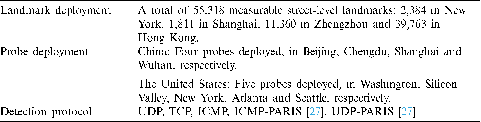
We conducted a total of more than 5,000 (lasting for 21 days) traceroute measurements on street-level landmarks (105,461) in China and the US by using nine probes in Beijing, Chengdu, Shanghai, Wuhan, Washington, Silicon Valley, New York, Atlanta and Seattle, and obtains a lot of delay information.
In order to verify the relationship between delay similarity and geographical distribution, we use the K-means algorithm to cluster the delay vectors of landmarks in China and US separately in this section. We selected cluster quantity K making the contour coefficient meet its maximum. When the numbers of clusters in China and the United States are 326 and 168 respectively, the contour coefficients reach its maximum, which are 0.72 and 0.83, respectively. The delay clustering results and geographical distribution statistical results of landmarks are shown in Tab. 1.
Table 1: Distribution of cluster quantity under different landmark coverage
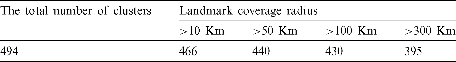
In Tab. 1, there are 395 clusters of landmarks with geographical distribution covering greater than 300 Km. Although the delays in these clusters are similar, the actual distance between the corresponding landmarks is greater than 300 Km, which means that the landmarks with similar delays are not necessarily geographically close.
In fact, among the above 494 clusters, the geographical locations where the landmarks in cluster W (a total of 315 landmarks), cluster X (124 landmarks), cluster Y (324 landmarks) and cluster Z (187 landmarks) are located are shown in Fig. 1. The landmarks in cluster W are located in Dallas, Houston, etc. in the United States. The landmarks in cluster X are located in Los Angeles, San Francisco, etc. in the United States. The landmarks in cluster Y are located in Shanghai, Hangzhou, etc. in China. The landmarks in cluster Z are located in Chengdu, Yibin, etc. in China. The average contour coefficients of cluster W, cluster X, cluster Y and cluster Z are 0.73, 0.76, 0.81 and 0.83, respectively. As a consequence, it is unreliable to merely use the similarity of delays as the basis for geolocation.
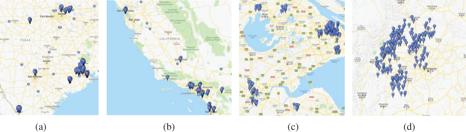
Figure 1: Geographical distribution of the landmarks with partial delay similarity. (a) Distribution of the landmarks in cluster W; (b) Distribution of the landmarks in cluster X. (c) Distribution of the landmarks in cluster Y; (d) Distribution of the landmarks in cluster Z
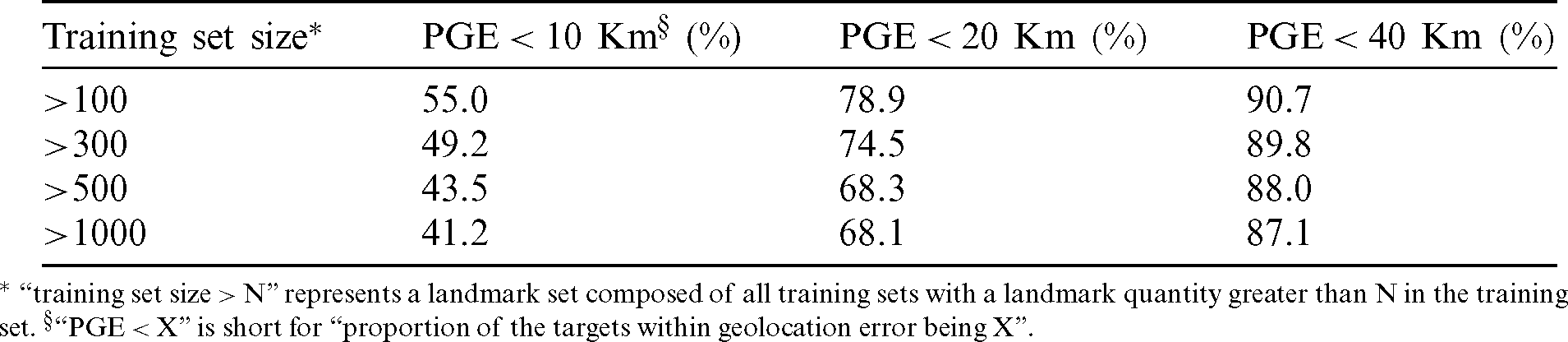
Fig. 2 shows the CDF (cumulative distribution function) of geolocation error when the TNN algorithm geolocates the targets in Shanghai, New York, Hong Kong and Zhengzhou. When the training size is greater than 100, 300, 500 and 1000, respectively, the geolocation median error is 9.2, 10.3, 12.2 and 12.9 Km. Tab. 2 shows the statistical results with the geolocation error being 10, 20 and 40 Km, respectively, when the TNN algorithm geolocates the targets.
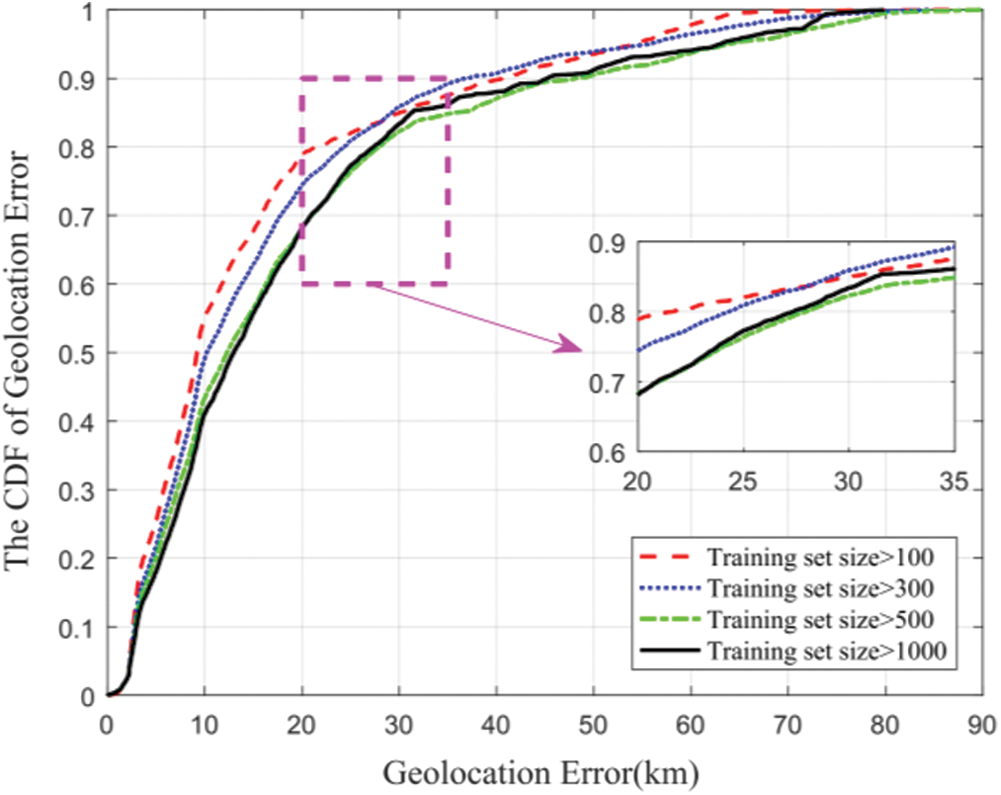
Figure 2: Error distribution of geolocation by the TNN algorithm
Table 2: The proportion of geolocation error of the TNN algorithm
* “ ” represents a landmark set composed of all training sets with a landmark quantity greater than N in the training set.
  “
“ ” is short for “proportion of the targets within geolocation error being X”.
Tab. 2 shows that the geolocation accuracy rate of the TNN algorithm with a geolocation error being 10, 20 and 40 Km, respectively, is not very high. This may be due to the fact that when the TNN algorithm trains the neural network with all landmarks, the landmark position of similar delay is not adjacent very often, so the mapping relationship between the delay and location of the landmarks learned by the neural network is not very strong.
3 Basic Principles and Main Steps of Proposed Algorithm
The basic idea of the algorithm is as follows: Based on the rule that hosts in the same local area and under the same network conditions often have similarity in their delays, the delays and relative hop counts are obtained for geolocation. The schematic framework of the algorithm is shown in Fig. 3.
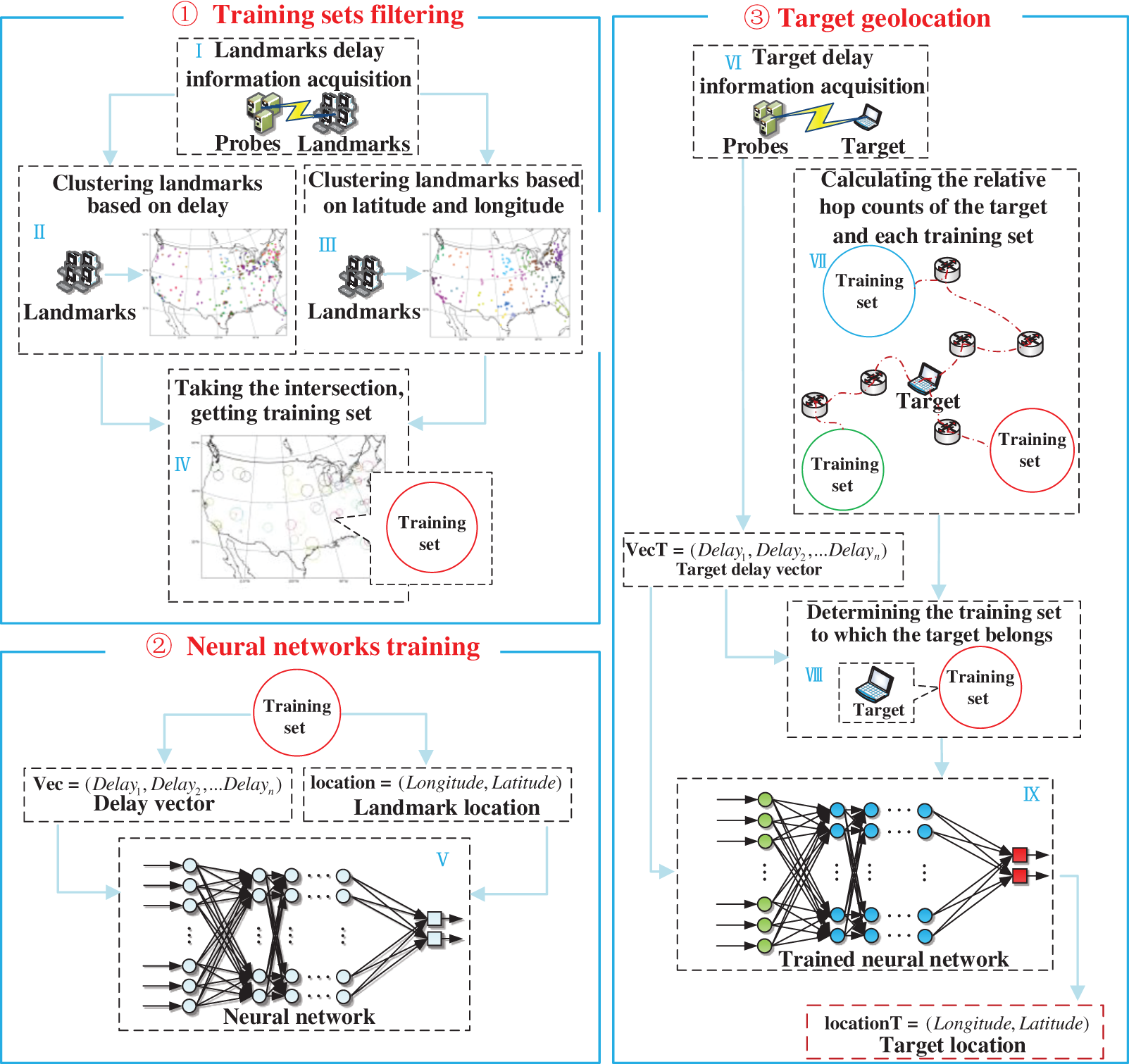
Figure 3: Algorithm frame diagram
As shown in Fig. 3, the algorithm is divided into three parts: ➀ Training sets filtering, ➁ Neural networks training, and ➂ Target geolocation. The specific steps of the algorithm are as follows:
➀ Training sets filtering. First, deploy n probes  , and acquire the delay from the probes to landmark sets, and construct absolute delay vectors:

where  represents the delay vector of the j-th landmark, and di, j represents the delay from the detection source i to the landmark j . Then, use Eq. (1) to cluster the landmarks. Next, use the latitude and longitude in the landmark set to cluster all the landmarks. Finally, the intersection of the two clustering results is calculated, and each intersection is used as a training set, so that the delay, latitude and longitude in each training set landmark are similar.
➁ Neural networks training. Take the delay of the landmarks in the training set Ci as input, and the latitude and longitude thereof as output, obtaining a well-trained neural network.
➂ Target geolocation. First, acquire the delay information from n probes to the target, express it as

where di represents the delay from the detection source i to the target. Then, Eq. (2) is used to determine the delay cluster which the target belongs to, calculate the training set having the smallest relative hop counts with target in the delay cluster, record the relative hop counts between target and the training set as V. Set the threshold U, and if  , input the neural network constructed by Cj in the Eq. (2) to obtain its latitude and longitude; otherwise, end the algorithm.
Among them, training sets filtering, neural network training and target geolocation are the important parts of the algorithm, which will be described in detail in the following subsections.
Because the geographical location of landmarks with similar delay is not necessarily close, and if all landmarks are used as training sets to train neural network, the result of location will be unreliable. Therefore, the training sets need to be filtered so that the delay, latitude and longitude of landmarks in each training set are similar. The specific steps are as follows:
Input: Delay vectors of landmarks, longitude and latitude of landmarks
Output: Filtered training sets
Step 1 Use Eq. (1) to perform K-means clustering on the landmarks, wherein K value is iterated in ascending order, and then select the k value maximizing the contour coefficient, and record the clustering set as  .
.
Step 2 Use the latitude and longitude in the landmark set to cluster all the landmarks, in terms of the number of clusters, also select the value corresponding to the maximum contour coefficient and recording it as h, and record the clustering set as  .
.
Step 3 Calculate  and record the final set of clusters as
  .
.
At this time, the delay, latitude and longitude of the landmarks in each training set are similar. The neural network is trained by using the landmarks in each training set, and the mapping between delay and latitude and longitude will be more reliable.
As a result, this training set can ensure that the samples with delay similarity are geographically close. Close geographical locations and delay similarity can indicate that the samples are similar in network local characteristics. For example, the samples have a common router, and the hop counts from them to the common router are not large, showing that these samples have very similar paths and thus share similarities in network characteristics such as network congestion. It is therefore reasonable to use the samples in such sets as training sets to train the neural networks.
Use Eq. (1) of the landmarks in Ci as the input of the neural network, and use the latitude and longitude vectors of the landmarks in Ci as the output of the neural network to train the neural network. This paper uses the multilayer perceptron neural network, and its structure is shown in Fig. 4 [24].
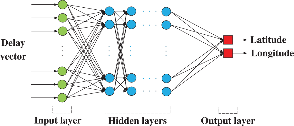
Figure 4: Neural network structural diagram
Among them, the number of hidden layers is n. The calculation formula of the output  of the hidden layer neuron j in the i-th layer is

where  is the output value of the hidden layer neuron k in the i −1 layer,
  is the connection weight from the hidden layer neuron k in the i −1 layer to the current layer neuron j,
  is the threshold of the hidden layer neuron j in the
  layer. Ik is the input value of the input layer neuron k. The hidden layer neuron activation function
  is set to a sigmoid function, which is just like

The calculation formula of the output layer neurons is

where  is the output value of the hidden layer neuron j in the n layer, wj, x and wj, y are the connection weights from the hidden layer neuron j in the n-th layer to the output layer neuron x and y,
  and
and  are the thresholds of the output layer neuron x and y.
After training the neural network for each training set, in target geolocation, it is first necessary to judge the training set to which the target belongs. Then, the target delay vector is input into the neural network trained by the training set to obtain the latitude and longitude of the target. Specific steps are as follows:
Input: Target IP
Output: Target longitude and latitude
Step 1 Use the detection source deployed in the previous stage to measure the delay of the target, and use the Ally method [25] and the Mercator [26] method to merge the router aliases. Construct Eq. (2) using targets. Record the hop counts of each router and the target in each measurement path.
Step 2 Calculate the Euclidean distance between the Di center and Eq. (2), and select the Di whose center has the smallest Euclidean distance with Eq. (2) as Di to which the target T belongs.
Step 3 Extract the router in the path of the set Cj in the probe measurement set Di, which is denoted as

where rm is the k-th router in Cj, and s is the number of routers in the path of the set Cj. The minimum hops of the distance between rm and the landmarks in Cj are recorded as hrm, Cj.
Step 4 By taking the intersection of routers in the probe-to-target paths and  , common router sets are obtained, which is denoted as

p is the number of common routers for  and the routers in the paths from probes to the target. The relative hop count of T and Cj is recorded as

where hrm, T is the minimum hops of the distance between rm and the target. Cj with the smallest Lj is used as the training set to locate the target, and record the smallest Lj as V.
Step 5 Set the threshold U, and if  , use the neural network formed by the training set Cj to geolocate the target; otherwise, end the algorithm.
The feasibility behind this strategy is as follows. The algorithm uses delay to determine the cluster to which the target belongs (clusters are obtained by time-delay clustering), but this cluster may produce multiple subclusters after the intersection with the cluster of latitude and longitude clustering. Therefore, it is necessary to calculate the relative hop count between the target and the landmarks in multiple clusters, and take the cluster with the smallest relative hop count as the target geolocation training set. It is worth noting that the “relative hop count between the target and the cluster” refers to the minimum relative hop count between the target and a landmark in the cluster, and to some extent, it represents the similarity between the target and the landmark. Specifically, the smaller the relative hop count, the more similar the target is to a certain sample in the cluster, and the mapping relationship between the target’s delay and latitude and longitude is more consistent with that of the trained neural network for this cluster. On the other hand, the greater the relative hop count, the greater the difference between the target and the sample path in this cluster. At this time, network characteristics such as path and congestion will affect the mapping relationship between delay and latitude and longitude, making the mapping relationship of the target different from that of trained neural network for this cluster. Consequently, in the algorithm, it is reasonable to measure the reliability of geolocation by setting a corresponding threshold. When the relative hop count is greater than the threshold, the algorithm deems that the target cannot be geolocated, thus ensuring the reliability of the algorithm under different geolocation requirements.
4 Experimental Results and Analysis
This section mainly verifies the rationality and effectiveness of the proposed algorithm. The experiment includes two experiments: Verification on the geolocation effect of the algorithm, and comparative verification. The experimental setups are shown in Tab. 3.
In Tab. 3, the landmarks used in the verification of the correlation between delay similarity and geographical distribution in Section 2 include the landmarks used in the verification on the geolocation effect of the algorithm and comparative verification.
Because the IRLD algorithm and NC-Geo algorithm belong to the geolocation under the specific conditions of the SLG algorithm. Unlike the application scenarios in this paper, the geolocation conditions of the SLG algorithm are more general, so comparative verification is carried out on the algorithm proposed in this paper and the SLG algorithm and TNN algorithm.
4.1 Verification on the Geolocation Effect of the Algorithm
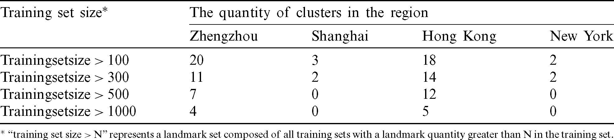
Based on the experimental setups in Tab. 3, we verify the effect of the geolocation algorithm in this subsection. 80% of the landmarks are randomly selected from each city as the candidate set of the training set for training network, and the remaining 20% of the landmarks (a total of 11,063) are used as unknown targets for geolocation verification. The landmarks can be divided into 67 clusters by using the landmark clustering in the algorithm and filtering algorithm. Tab. 4 shows the relationship between the size of the training set, the number of clusters and the geographical location thereof.
Table 4: Size of the training set and the statistical table of cluster quantity distribution
* “ ” represents a landmark set composed of all training sets with a landmark quantity greater than N in the training set.
Tab. 5 shows the geolocation effects of training sets in different training sizes and different geolocation thresholds on the corresponding targets.
Table 5: Relationship between different training set sizes, different thresholds and the quantity of the targets that can be geolocated and geolocation error
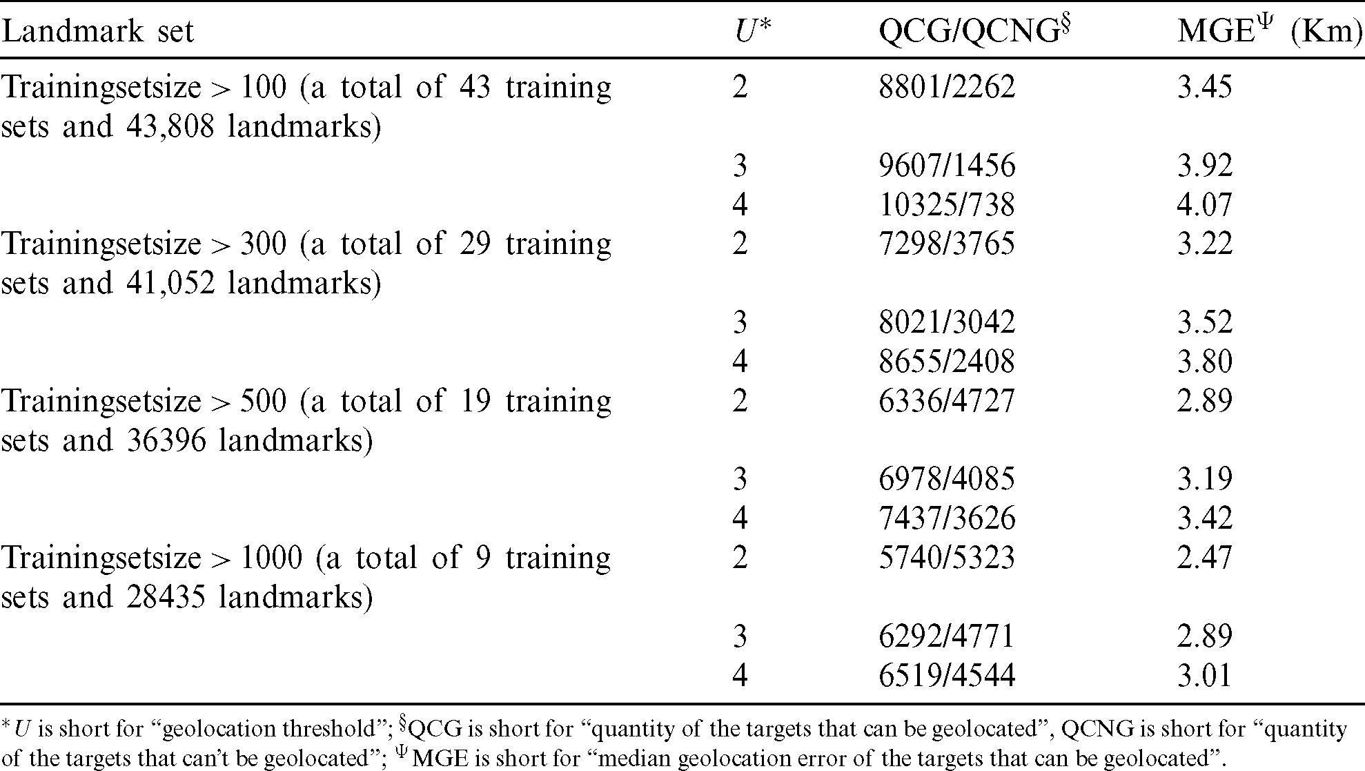
*U is short for “geolocation threshold”;  QCG is short for “quantity of the targets that can be geolocated”, QCNG is short for “quantity of the targets that can’t be geolocated”;
  MGE is short for “median geolocation error of the targets that can be geolocated”.
Fig. 5 shows the geolocation error cumulative distribution of the targets that can be geolocated under different training set sizes and different threshold conditions. The red dashed line, blue dot line, green chain line and the black solid line indicate the cumulative error distribution of all neural networks formed by the training sets with the landmarks greater than 100, 300, 500 and 1000 in each training set for the corresponding target geolocation, respectively.
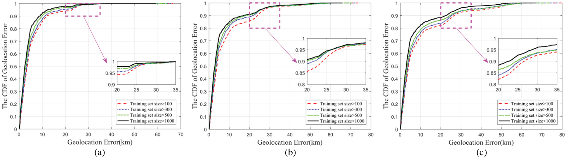
Figure 5: The CDF of geolocation error under different training set sizes and thresholds. (a) Threshold is 2. (b) Threshold is 3. (c) Threshold is 4
Tab. 5 and Fig. 5 show that as the total number of landmarks in the landmark set decreases, the number of samples in a single training set increases, and the number of targets that can be geolocated decreases, but the geolocation error (median error/maximum error) is on a downward trend. The reason lies in that the network trained by the training set that fails to satisfy a certain number of samples lacks universality, which is statistically reasonable. In addition, it can be seen that different geolocation thresholds have different degrees of influence on the number of targets that can be geolocated and geolocation error. As the geolocation threshold increases, the number of targets that can be geolocated increases, but the geolocation error also increases.
It can be seen that the geolocation effect of the algorithm is closely related to the number of samples in the training set and the geolocation threshold. In fact, it is also closely related to the network characteristics of the geolocation target and the training set.
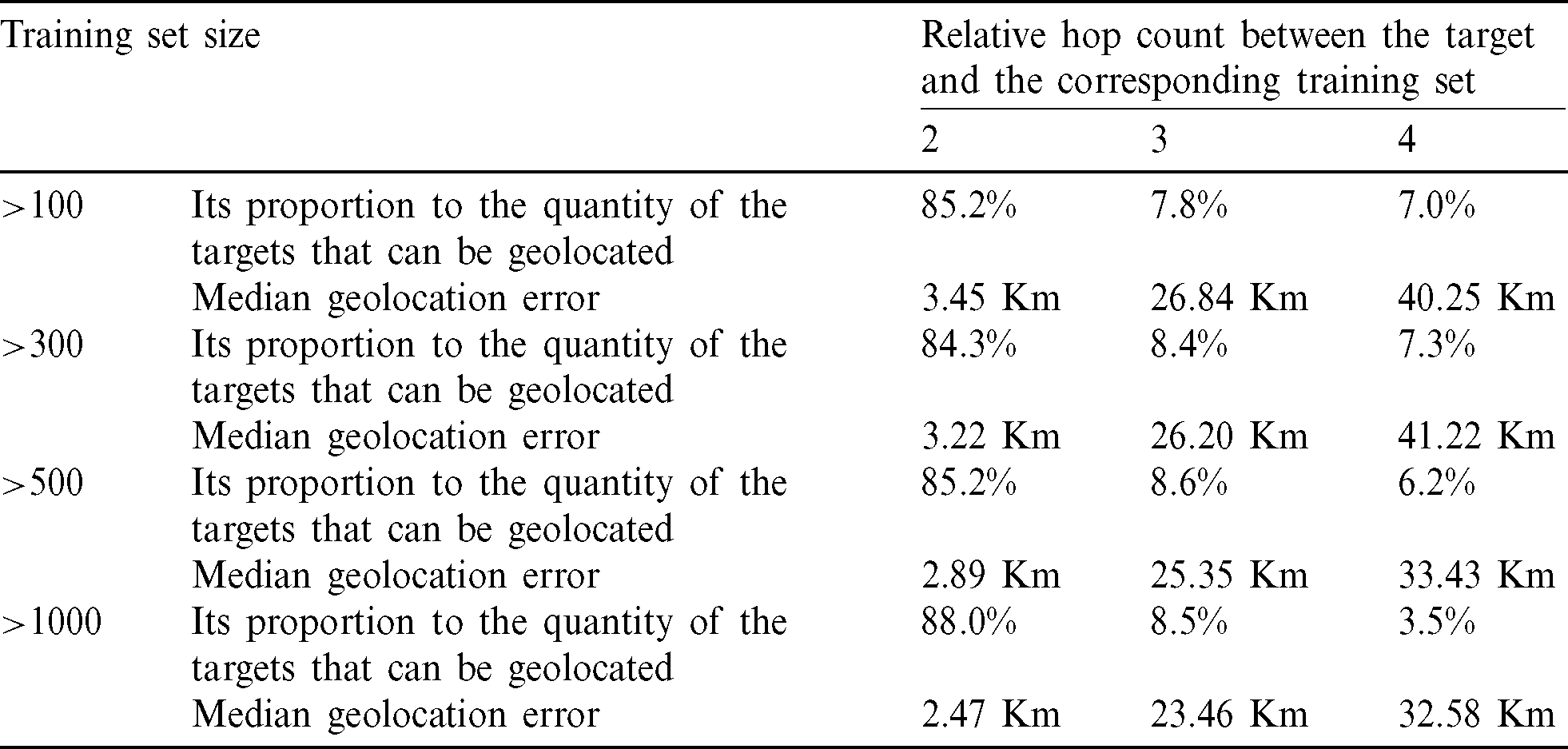
Tab. 6 shows the number of targets that can be geolocated, geolocation error and other geolocation effect when the number of landmarks in the corresponding training sets in Zhengzhou and Hong Kong and the geolocation threshold are 4.
Table 6: Geolocation effect under different training sets when the threshold is 4
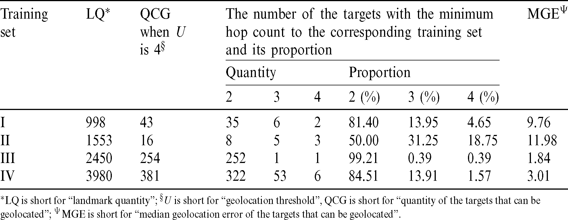
*LQ is short for “landmark quantity”;  is short for “geolocation threshold”, QCG is short for “quantity of the targets that can be geolocated”;
  MGE is short for “median geolocation error of the targets that can be geolocated”.
Tab. 6 shows that under the same threshold condition, the smaller the relative hop count from the target to the corresponding training set, the higher its proportion in the whole targets that can be geolocated, and the higher the geolocation accuracy. This, to some extent, shows that the smaller the hop count from the target to the training set, the more similar the network characteristics of the target are to the network characteristics of the landmark in the training set. Thus, the use of the geolocation algorithm should fully consider the relative hop count from the target to the training set and the sample quantity of the training set.
In this subsection, we compare the geolocation effect of the proposed algorithm in this paper with those of the SLG algorithm and the TNN algorithm under the situations of the same target and landmark.
Fig. 6 shows the geolocation cumulative distribution of the proposed algorithm in this paper, the SLG algorithm and the TNN algorithm. The black line, red dashed line and blue dot line indicate the geolocation error cumulative distribution of the proposed algorithm, SLG algorithm and TNN algorithm, respectively. It can be seen from the geolocation error cumulative distribution in the Fig. 6 that when the geolocation threshold is 2 or 3, the geolocation effect of the proposed algorithm is better than those of the SLG algorithm and TNN algorithm, but when the threshold is 4, the partial geolocation result of the proposed algorithm is weaker than that of the TNN algorithm.
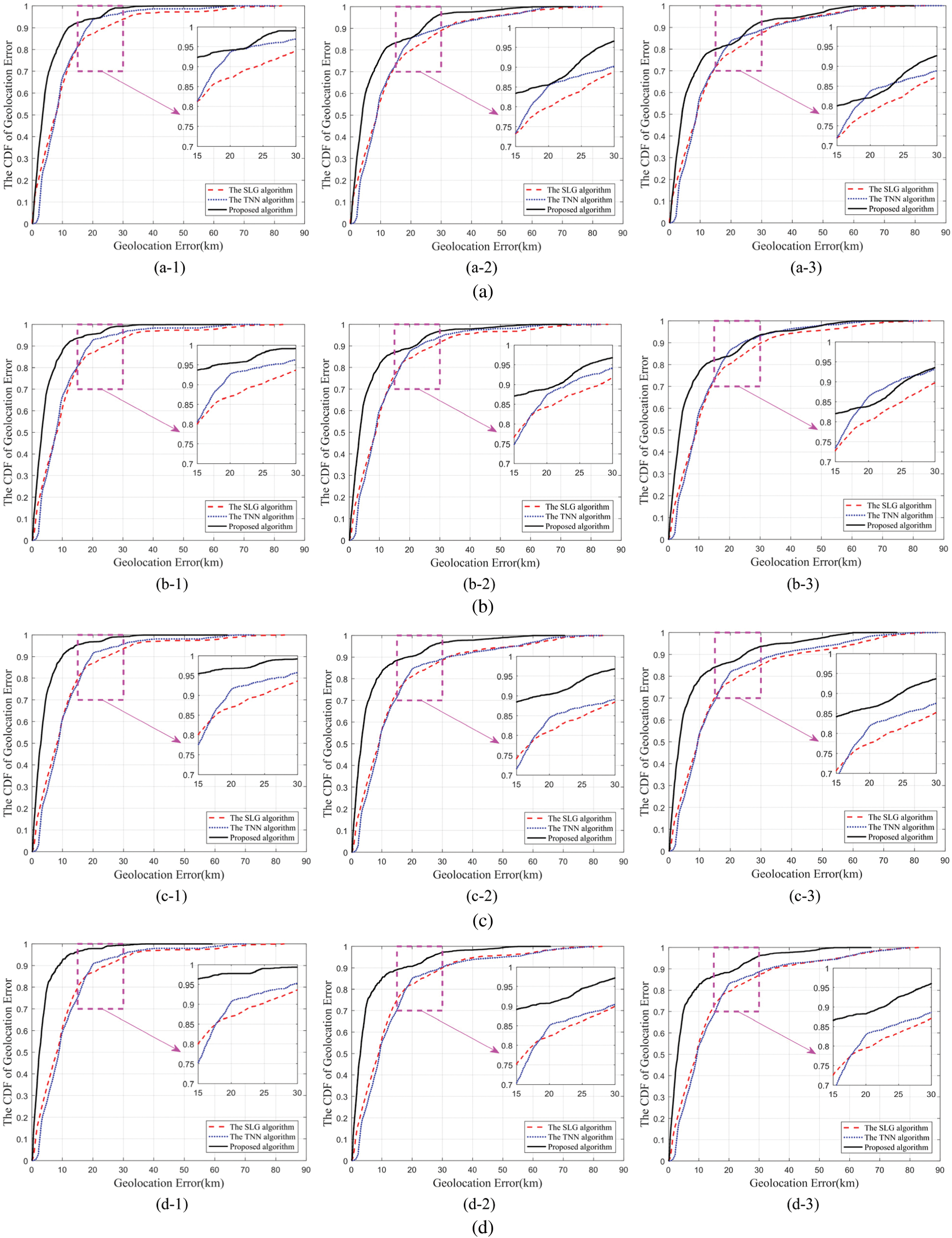
Figure 6: Comparison on IP geolocation error under the same conditions. (a) Geolocation error comparison when the training  . (a-1) Threshold is 2. (a-2) Threshold is 3. (a-3) Threshold is 4. (b) Geolocation error comparison when the training
  . (b-1) Threshold is 2. (b-2) Threshold is 3. (b-3) Threshold is 4. (c) Geolocation error comparison when the training
  . (c-1) Threshold is 2. (c-2) Threshold is 3. (c-3) Threshold is 4. (d) Geolocation error comparison when the training set
  . (d-1) Threshold is 2. (d-2) Threshold is 3. (d-3) Threshold is 4
Tab. 7 shows with a geolocation threshold being 4, the statistical results of the proposed algorithm in this paper, the SLG algorithm and TNN algorithm when the geolocation error is 10, 20 and 40 Km.
Table 7: The proportion of geolocation error when the threshold is 4
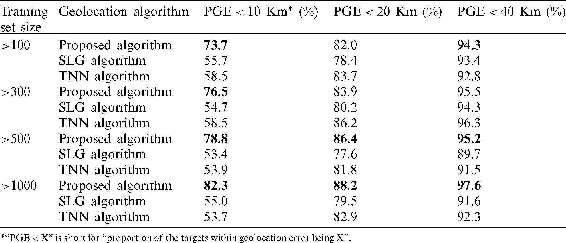
Tab. 7 shows that when the landmarks are composed of a training set with training samples greater than 100, the geolocation accuracy rate of the algorithm within 20 Km is 82.0%, while the geolocation accuracy rate of the TNN algorithm is 83.7%.
When the landmarks are composed of a training set with training samples greater than 300, the geolocation accuracy rates of the algorithm within 20 and 40 Km are 83.9% and 95.5%, respectively, while the geolocation accuracy rates of the TNN algorithm are 86.2% and 96.3%, respectively. Tab. 8 gives the reasons for this phenomenon.
Table 8: Relationship between the proportion of different relative hop count between the target and the corresponding training set and the geolocation error under different training set sizes
Tab. 8 shows that when the relative hop count between the target and the training set is relatively large, the neural network trained by the training set is not sufficient to reflect the network characteristics of the target, which may increase the error. The TNN algorithm uses all landmarks as a training set, which blurs local network characteristics. However, the TNN algorithm will not guarantee higher geolocation reliability.
Section 2 shows the geolocation of all targets by TNN algorithm. Fig. 2 shows that when the TNN algorithm geolocates the targets that it considers can be geolocated, although the number of targets that can be geolocated is more than the proposed algorithm in this paper, its geolocation error increases significantly. Tab. 2 shows that the geolocation accuracy rate of the TNN algorithm with a geolocation error being 10, 20 and 40 Km, respectively, is significantly lower than that of the proposed algorithm. Hence, it can be seen that the proposed algorithm in this paper is of greater reliability.
IP geolocation algorithm based on delay similarity is a kind of classical IP geolocation algorithms. However, owing to the inconsistency between IP similar delays and geographical similarity, the reliability of the geolocation results of such algorithms is not enough. Aiming at the deficiencies in this kind of algorithm, this paper proposes a street-level geolocation algorithm based on landmarks clustering. This paper has carried out experimental verification on a total of 55,318 measurable street-level landmarks in Hong Kong, Shanghai, Zhengzhou and New York. The experimental results show that the proposed algorithm achieves street-level geolocation, and the reliability of the street-level geolocation algorithm is improved effectively compared with the SLG algorithm and TNN algorithm.
Because the delays from the probes to the hosts are not stable enough during network measurement, the geolocation result would be affected, and the path of the network measurement is stable. Infuture work, we consider integrating path vectorization into the construction of geolocation model to improve the geolocation accuracy.
Acknowledgement: The authors are grateful to Ruixiang Li of Zhengzhou Science and Technology Institute for providing landmarks for our experiment. The authors are grateful to Haoyu Lu of Zhengzhou Science and Technology Institute for polishing the paper.
Funding Statement: This work was supported by the National Key R&D Program of China 2016YFB0801303 (F. L. received the grant, the sponsors’ website is https://service.most.gov.cn/); by the National Key R&D Program of China 2016QY01W0105 (X. L. received the grant, the sponsors’ website is https://service.most.gov.cn/); by the National Natural Science Foundation of China U1636219 (X. L. received the grant, the sponsors’ website is http://www.nsfc.gov.cn/); by the National Natural Science Foundation of China 61602508 (J. L. received the grant, the sponsors’ website is http://www.nsfc.gov.cn/); by the National Natural Science Foundation of China 61772549 (F. L. received the grant, the sponsors’ website is http://www.nsfc.gov.cn/); by the National Natural Science Foundation of China U1736214 (F. L. received the grant, the sponsors’ website is http://www.nsfc.gov.cn/); by the National Natural Science Foundation of China U1804263 (X. L. received the grant, the sponsors’ website is http://www.nsfc.gov.cn/); by the Science and Technology Innovation Talent Project of Henan Province 184200510018 (X. L. received the grant, the sponsors’ website is http://www.hnkjt.gov.cn/).
Conflicts of Interest: The authors declare that they have no conflicts of interest to report regarding the present study.
1 J. A. Muir and P. C. V. Oorschot. (2009). “Internet geolocation: Evasion and counterevasion,” ACM Computing Surveys, vol. 42, no. 1, pp. 1–23. [Google Scholar]
2 O. Dan, V. Parikh and B. D. Davison. (2016). “Improving IP geolocation using query logs,” in Proc. ACM Int. Conf. on Web Search and Data Mining, New York, NY, USA, pp. 347–356. [Google Scholar]
3 R. Li, Y. Liu, Y. Qiao, T. Ma, B. Wang. (2019). et al., “Street-level landmarks acquisition based on SVM classifiers,” Computers, Materials and Continua, vol. 59, no. 2, pp. 591–606.
4 Y. Wang, Y. Sun, S. Su, Z. Tian, M. Li. (2019). et al., “Location privacy in device-dependent location-based services: Challenges and solution,” Computers, Materials & Continua, vol. 59, no. 3, pp. 983–993. [Google Scholar]
5 Y. Liu, Z. Yang, X. Yan, G. Liu and B. Hu. (2019). “A novel multi-hop algorithm for wireless network with unevenly distributed nodes,” Computers, Materials & Continua, vol. 58, no. 1, pp. 79–100. [Google Scholar]
6 V. N. Padmanabhan and L. Subramanian. (2001). “An investigation of geographic mapping techniques for internet hosts,” ACM SIGCOMM Computer Communication Review, vol. 31, no. 4, pp. 173–185. [Google Scholar]
7 Whois. (2020). “Whois lookup,” . [Online]. Available: www.whois.net. [Google Scholar]
8 IP2location. (2020). “Identify geographical location by IP address,” . [Online]. Available: www.ip2location.com. [Google Scholar]
9 Maxmind. (2020). “Detect online fraud and locate online visitors,” . [Online]. Available: www.maxmind.com. [Google Scholar]
10 Y. Shavitt and N. Zilberman. (2011). “A geolocation databases study,” IEEE Journal on Selected Areas in Communications, vol. 29, no. 10, pp. 2044–2056. [Google Scholar]
11 I. Poese, S. Uhlig, M. A. Kaafar, B. Donnet and B. Gueye. (2011). “IP geolocation databases: Unreliable?,” ACM SIGCOMM Computer Communication Review, vol. 41, no. 2, pp. 53–56. [Google Scholar]
12 B. Gueye, A. Ziviani, M. Crovella and S. Fdida. (2006). “Constraint-based geolocation of internet hosts,” IEEE/ACM Transactions on Networking, vol. 14, no. 6, pp. 1219–1232. [Google Scholar]
13 B. Wong, I. Stoyanov and E. G. Sirer. (2007). “Octant: A comprehensive framework for the geolocalization of internet hosts,” in Proc. Sym. on Networked System Design and Implementation, Cambridge, Massachusetts, USA, pp. 313–326. [Google Scholar]
14 M. J. Arif, S. Karunasekera and S. Kulkarni. (2010). “GeoWeight: Internet host geolocation based on a probability model for latency measurements,” in Proc. Australasian Conf. on Computer Science, Brisbane, Queensland, Australia, pp. 89–98. [Google Scholar]
15 B. Eriksson, P. Barford, J. Sommers and R. Nowak. (2010). “A learning-based approach for IP geolocation,” in Proc. Int. Conf. on Passive and Active Network Measurement, Zurich, Switzerland, pp. 171–180. [Google Scholar]
16 S. Liu, F. Liu, F. Zhao, L. Chai and X. Luo. (2016). “IP city-level geolocation based on the PoP-level network topology analysis,” in Proc. Passive and Active Measurement, Hatfield, UK, pp. 109–114. [Google Scholar]
17 G. Zhu, X. Luo, F. Liu and F. Zhao. (2016). “City-level geolocation algorithm of network entities based on landmark clustering,” in Proc. Int. Conf. on Advanced Communication Technology, Pyeongchang, South Korea, pp. 306–309. [Google Scholar]
18 F. Yuan, F. Liu, D. Huang, Y. Liu and X. Luo. (2019). “A high completeness PoP partition algorithm for IP geolocation,” IEEE Access, vol. 7, pp. 28340–28355. [Google Scholar]
19 S. Zu, X. Luo, S. Liu, Y. Liu and F. Liu. (2018). “City-level IP geolocation algorithm based on PoP network topology,” IEEE Access, vol. 6, pp. 64867–64875. [Google Scholar]
20 Y. Wang, D. Burgener, M. Flores, A. Kuzmanovic and C. Huang. (2011). “Towards street-level client independent IP geolocation,” in Proc. USENIX Conf. on Networked Systems Design and Implementation, Boston, MA, USA, pp. 365–379. [Google Scholar]
21 F. Zhao, X. Luo, Y. Gan, S. Zu, Q. Cheng. (2018). et al., “IP geolocation based on identification routers and local delay distribution similarity,” Concurrency and Computation: Practice and Experience, vol. 31, no. 22, pp. e4722.1–e4722.15. [Google Scholar]
22 J. Chen, F. Liu, Y. Shi and X. Luo. (2018). “Towards IP location estimation using the nearest common router,” Journal of Internet Technology, vol. 19, no. 7, pp. 2097–2110. [Google Scholar]
23 H. Jiang, Y. Liu and J. N. Matthews. (2016). “IP geolocation estimation using neural networks with stable landmarks,” in Proc. IEEE Conf. on Computer Communications Workshops, San Francisco, CA, USA, pp. 170–175. [Google Scholar]
24 R. P. Lippmann. (1989). “Pattern classification using neural networks,” IEEE Communications Magazine, vol. 27, no. 11, pp. 47–50. [Google Scholar]
25 B. Eriksson, P. Barford and R. Nowak. (2008). “Network discovery from passive measurements,” ACM SIGCOMM Computer Communication Review, vol. 38, no. 4, pp. 291–302. [Google Scholar]
26 R. Govindan and H. Tangmunarunkit. (2000). “Heuristics for internet map discovery,” in Pro. Annual Joint Conf. of the IEEE Computer and Communications Societies, Tel Aviv, Israel, pp. 1371–1380. [Google Scholar]
27 B. Augustin, X. Cuvellier, B. Orgogozo, F. Viger, T. Friedman. (2006). et al., “Avoiding traceroute anomalies with Paris traceroute,” in Proc. ACM SIGCOMM Conf. on Internet Measurement, New York, NY, USA, pp. 153–158.
 | This work is licensed under a Creative Commons Attribution 4.0 International License, which permits unrestricted use, distribution, and reproduction in any medium, provided the original work is properly cited. |