DOI:10.32604/cmc.2021.013966
| Computers, Materials & Continua DOI:10.32604/cmc.2021.013966 | |
| Article |
An Efficient False-Positive Reduction System for Cerebral Microbleeds Detection
1Department of Computer Science, COMSATS University Islamabad, Attock Campus, Attock, Pakistan
2Department of Media Design and Technology, Faculty of Engineering & Informatics, University of Bradford, Bradford, BD7 1AZ, UK
3Department of Smart Device Engineering, School of Intelligent Mechatronics Engineering, Sejong University, Seoul, South Korea
4School of Computer Art, College of Art & Technology, Chung-Ang University, Anseong, 17546, South Korea
*Corresponding Author: Muazzam Maqsood. Email: muazzam.maqsood@cuiatk.edu.pk
Received: 27 August 2020; Accepted: 26 September 2020
Abstract: Cerebral Microbleeds (CMBs) are microhemorrhages caused by certain abnormalities of brain vessels. CMBs can be found in people with Traumatic Brain Injury (TBI), Alzheimer’s disease, and in old individuals having a brain injury. Current research reveals that CMBs can be highly dangerous for individuals having dementia and stroke. The CMBs seriously impact individuals’ life which makes it crucial to recognize the CMBs in its initial phase to stop deterioration and to assist individuals to have a normal life. The existing work report good results but often ignores false-positive’s perspective for this research area. In this paper, an efficient approach is presented to detect CMBs from the Susceptibility Weighted Images (SWI). The proposed framework consists of four main phases (i) making clusters of brain Magnetic Resonance Imaging (MRI) using k-mean classifier (ii) reduce false positives for better classification results (iii) discriminative feature extraction specific to CMBs (iv) classification using a five layers convolutional neural network (CNN). The proposed method is evaluated on a public dataset available for 20 subjects. The proposed system shows an accuracy of 98.9% and a 1.1% false-positive rate value. The results show the superiority of the proposed work as compared to existing states of the art methods.
Keywords: Microbleeds detection; false-positive; deep learning; CNN
Cerebral Microbleeds (CMBs) are chronic body fluid products having minor weights that are often found in patients. Such patients are tormented by different diseases including TBI, Alzheimer’s Disease (AD), and stroke [1]. The position of these CMBs shows etiology. The amount of these CMBs can specify the severity of the possible cognitive impairment and intracerebral hemorrhage (ICH) [2]. Deep CMBs in the thalamus are characteristically connected with hypertension, while the occurrence of labor CMBs may also recommend cerebral amyloid angiopathy. These are the conditions in which protein components in the brain amyloid starts building up in the cerebral [3]. Identifying CMBs could be medically critical to evaluate the advantages as well as threats in antitoxic medicine preparation for patients specifically having stroke ailment [1]. Finally, the detection of CMBs is important for AD and TBI diagnosis and prognosis.
Worldwide, probably more than 49-million individuals are getting TBI yearly [4]. In TBI, the high-level occurrence of microbleeds makes it important to observe this disease [5]. Therefore, correct, error-free, and consistent recognition of these microbleeds is crucial. Early and accurate diagnosis of the CMBs is still an open research area due to the difficult nature of this problem and its impact on human life. Hence, early and timely detection of CMBs is critical. As there are a lot of advancements in clinical diagnostics approaches, small or insignificant units in the cerebral can be easily anticipated which are helpful in CMBs diagnosis [3]. Furthermore, manual segmentation and identification of microbleeds remain a difficult and time-consuming task especially when the number of patients is very high. It is often noticed that manual segmentation results in false-positive due to the small sizes of CMB and similar structure of healthy tissues. Further, a neuroimage may contain more than one CMB. To detect these CMBs, usually MRI is usually used but SWI is extensively utilized for detecting CMBs [6].
In SWI, weighting masks of susceptibility are produced from high filtered images and then multiplied with the magnitude of images to generate complex images. The CMBs are minor sphere-shaped or oval sections with very little intensity on SWI images [7]. There are numerous kinds of CMB, like veins in the brain, blood, deposition of iron, and signal void because of low flow compensation [8]. Therefore, to detect CMBs manually can be inefficient and error-prone which can be handled by utilizing automatic CMB recognition algorithms. Generally, a two-phase algorithm is used for automatic detection of CMB, where the first stage is for candidate stage detection followed by the classification phase for reducing false-positive. There are various methods used for CMB detection recently that include both handcrafted feature selection methods and the end to end deep learning methods. Both these methods have their advantages and limitations as well. The CMB present in an image is usually extremely small and often face false-positive issue due to similar objects present in the image. The end to end deep learning methods are usually expensive in terms of computational cost and require a huge amount of labeled data especially for semantic segmentation. Therefore, there is a need to divide this problem into multiple steps to reduce false-positive which should be the focus of CMB detection methods.
From this line of research, in this study, an automatic approach is proposed for CMBs detection by using SWI MRI images. The main goal is to build up a framework having an option to accomplish high sensitivity. We show that with data pre-processing, the model gives high sensitivity value with few false positives, and outperformed both manually extracted, and existing single-direct framework. To overcome the limitation of currently proposed approaches, we have explored a wide variety of features including the textual and statistical-based features. These features are based on size, geometry, and transform that differentiate CMBs from other structures. The proposed approach consists of pre-processing from brain extraction, Region of Interest extraction by using the k-mean algorithm, feature extraction, post-processing to minimize the false positives, and classification using CNN. The proposed method is evaluated on a set of 20 subjects with 167 CMBs in total. The proposed approach has the following contributions:
• A segmentation-based approach is used to extract the most effective features relevant to CMB
• We explore different textual, statistical, and shape-based features in combination with deep learning for an efficient CMB detection method
• An efficient method is proposed to minimize false-positive to improve the performance of CMB detection
The rest of the paper is organized as follows: Section 2 summarizes the related work, Section 3 presents methodology, Section 4 explains results followed by the conclusion.
Many research groups have proposed an automated technique to detect CMB using different machine learning-based algorithms. Most of the techniques are a combination of segmentation and feature extraction from images. Lu et al. [9] proposed an approach to detect CMBs from the MRI by applying machine learning algorithms. They achieved a performance accuracy of 90% with 93.0% sensitivity. Hong et al. [10] used applied machine learning-based approaches by using the principal component analysis to reduce the feature size. They applied a shallow neural network by backpropagation to predict the CMBs and Non-CMBs and achieved an accuracy of 88.43%. Bian et al. [11] applied a 2-dimensional radial symmetry transform on the low-intensity projections of SWI images and utilized shape features to reduce false and achieved 86.5% sensitivity with 44.9 false positives per individuals. Tao et al. [12] proposed a Genetic Algorithm (GA) with a backpropagation neural network approach to distinguish the microbleed part from the non-microbleed parts and achieved an accuracy of 72.90%. Gagnon et al. [13] applied machine learning-based approaches by using entropy measure and naïve base classifiers to discriminate the CMBs and achieved 76.9% accuracy. Ourselin et al. [14] utilized RST to detect the microbleeds and then applied a machine learning classifier named random forest for classification and achieved 86% sensitivity.
Zhang et al. [15] utilized one hidden layer neural network with ReLU layers as an activation function to diagnose microbleeds in the brain MRI and achieved an accuracy of 93.05%. Fazlollahi et al. [16] proposed a random forest (RF) framework and achieved a 92.0% sensitivity with almost 16.8 false positives per individual. Van den Heuvel et al. [17] also proposed a RF framework with shape-based features for diagnosis of bleeds in TBI and achieved 89.1% sensitivity with almost 25.9 per subject false positives. Though great sensitivity could be certainly attained in the initial phase in the second phase, the performance is generally poor, leading to so many false positives. For example, Barnes et al. [18] established a machine learning framework center on the SVM with shape as well as intensity features and performed manual false-positive removal. Due to the difference in CMB’s shape and intensities on SWI images, effective designs and robust features are important. This can be minimized by utilizing a CNN, which has expressively enhanced the performance of object detection in the field of computer vision [5,19].
Dou et al. [20] proposed a CNN based framework by utilizing SWI images and achieved 93.2% sensitivity with the false-positive per subject is 2.7. Chen et al. [21] proposed a more multifaceted residual network using SWI images obtained at 7T and achieved 94.7%, sensitivity with 11.6 false positives. The low accuracy or a huge number of false positives of these techniques is halfway brought about by depending on SWI images alone. Especially, separating blood products is troublesome since CMBs and other blood cells are dim/unclear on SWI images. Furthermore, the value of contrast in SWI data is reliant on imaging parameters, particularly on a primary field value. These issues can be tackled by utilizing both size and magnitude of the image with normalization [22]. Utilizing the k-mean classifier to make clusters from stage images and reduce false-positive by using magnitude and area of CMB, for example, microbleeds can be isolated from paramagnetic blood items dependent on the area.
The vast majority to automatically recognize techniques for CMB utilizes a pre-determined number of features dependent on the shape, size, and intensity data. These features are insufficient to identify the CMBs complex nature. When these methods are compared with previously mentioned strategies, the proposed technique investigated a large feature-set to attain better performance. This proposed automatic approach for the detection of CMB framework comprises three stages, i.e., skull stripping, selecting initial candidate, Post-processing to reduce false positives, and used CNN for classification.
The primary purpose of the high false-positive rate in the detection of CMB is complex from the skull in MRI examines. The classification phase gets frequently confused and mixes the skull part with CMBs. Therefore, an appropriate approach of skull stripping in the pre-processing step is exceptionally significant for an efficient diagnosis of CMBs. An efficient skull stripping in the pre-processing step brings about an extensive decrease in the number of false positives. In contrast to prior techniques, the proposed method does not require much pre-processing.
The steps in pre-processing are just constrained to skull-removing from T2*—weighted neuroimages by utilizing the BrainSuite Tool. Fig. 1 illustrates the general flow diagram of the proposed methodology. The initial step of the methodology is to remove the skull from the actual brain part because this skull part increases the false-positive rate. After skull stripping, the best candidate region is chosen from the k-mean cluster, and post-processing is applied to discriminate true CMBs from false positives.
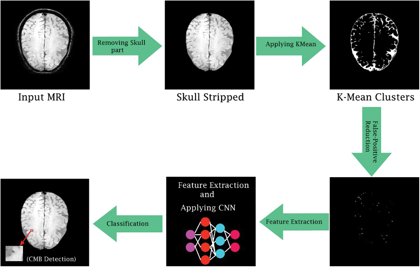
Figure 1: General flow diagram of the proposed framework
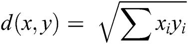
The preprocessed SWI brain image after removing the skull area, contains a lot of connected component CMBs and false positives. Therefore, the k-mean clustering approach is proposed to overcome these connected component issues. Conventional k-mean clustering is chosen where all the clusters are completely reliant on a first center point that was selected initially. K-mean accepts Euclidean distance as shown in Eq. (1) on which the clustering is performed by calculating similarity as well as a dissimilarity measure. At first center point for the k-mean grouping is randomly picked for the whole image and then distance amongst all pixels of an image is calculated. Pixels that have minimum distance value from the individual center point are clustered together. This loop continues until a new mean value is determined which then becomes centroid. This procedure converges until no change or alteration of value in the mean of the image is observed. The proposed approach instates its center point by centroid determination strategy as given in Eq. (2).
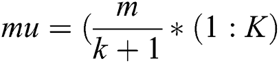
where k shows how many numbers of clusters will be formed, m represents the highest estimation of a pixel in MRI, and the value of k varies from 1 to K. The center point determination procedure works by guaranteeing major distinction between estimations of instated point, making it progressively efficient and robust by congregating to the last point in minimum loops.
False-positive means that you get a positive outcome for a negative value. These false positives create a problem, especially when it comes to clinical images. The k-mean from the previous phase provides an underlying segmentation of microbleeds. K-mean has a limitation as the CMBs are so tiny in size that it can easily be confused with other brain normal tissues. For this reason, some changes are required to reduce false positives from clusters produced by the k-mean algorithm. In our proposed work, we have performed this step before feature extraction and classification which helps us to reduce the false-positive rate significantly. The removal of false-positive is achieved by the removal of connected components and shape-based regions.
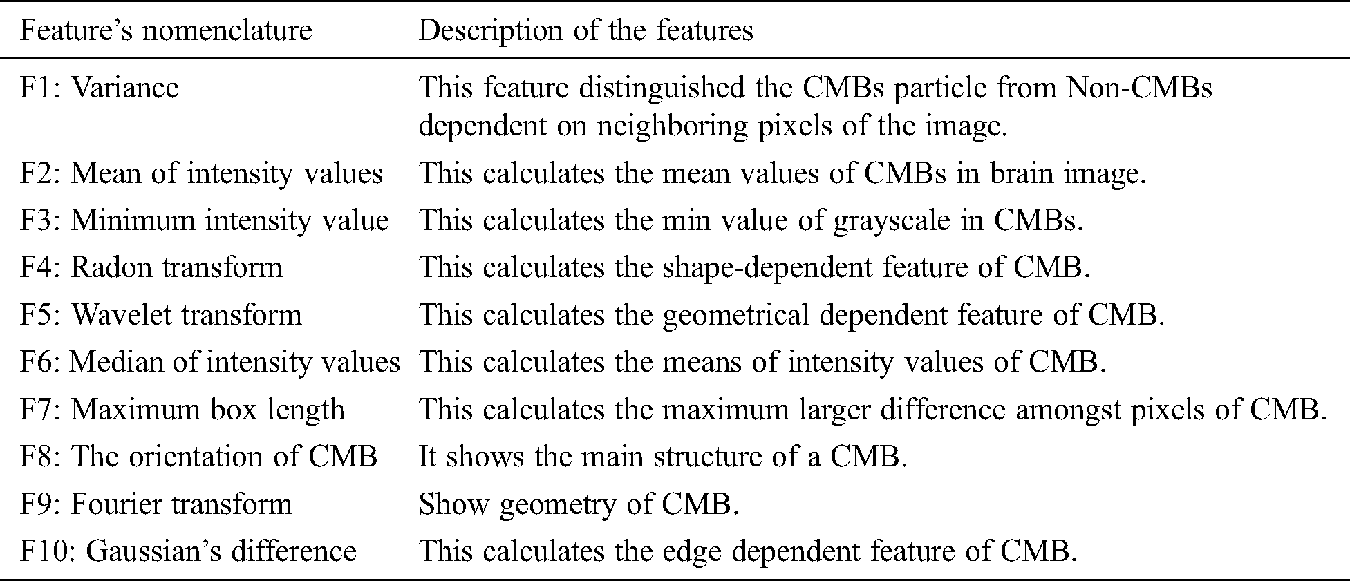
The post-processed data is acquired by removing the false-positive step. In the next step, the data is then forwarded to the feature extraction phase where different statistical, geometric, and local shape-dependent features were extracted and stored in a feature vector file. A brief description of the extracted feature is given in the below subsection. Tab. 1 shows the description of a distinct feature that we extracted in this study.
3.4.1 Gray-Level-Occurrence-Matrix
GLCM is a co-occurrence framework and it is characterized over an image to be the appropriation of co-existing values at a given set. The GLCM is ascertained how frequently a pixel with the dark level value i occur in an image either horizontally or vertically to neighboring pixels of value j. In GLCM, the number of gray levels is equal to the number of rows and columns of pixels in an image.
In this study, we use a large number of intensity levels of GLCM, i.e., g × g for every combination of (x, y). The formulation of GLCM in detecting pixels values of CMBs is illustrated in Fig. 2 for different gray levels. The GLCM matrix has further different features such as entropy, correlation, and homogeneity.
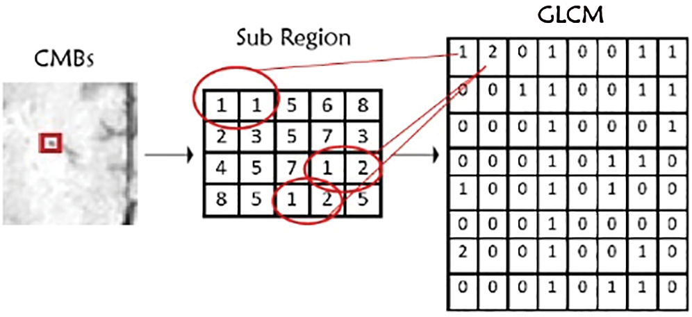
Figure 2: Gray-level-co-occurrence-matrix features illustration
The entropy determines the pattern store in the image that is required for compression of data images. This feature determines the data loss and it also calculates information in an image. It can be calculated as shown in Eq. (3).

This feature quantifies the direct dependence of the dark gray level of neighboring pixels in an image. The digital correlation of image is an optical procedure that utilizes tracking and recording of image system for an accurate 2 Dimensional and 3-Dimensional analysis of variations.
This is typically practiced by calculating the displacement, strain, and optical stream. However, it is generally applied in numerous domains of science and image processing. It can be calculated as shown in Eq. (4).
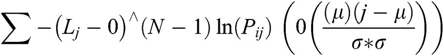
where, Pij shows the elements I,j of normalized-symmetrical GLCM, N represents the number of grayscale in the image, µ represents the mean value of GLCM and σ is the value of variance in referencing pixel of the image in GLCM matrix.
In numerous classification tasks, the CNN has been successful in imaging as well as text data classification. In this study, after extracting features from CMB and non-CMB part of brain MRI, we applied five layers CNN to classify the model. We utilized different hyperparameters and tuning of parameters to achieve excellent performance results. Our proposed overall architecture of CNN is shown in Fig. 3 where the extracted feature vector is passed to different convolutional layers along with filters to distinguish CMBs from Non-CMBs.
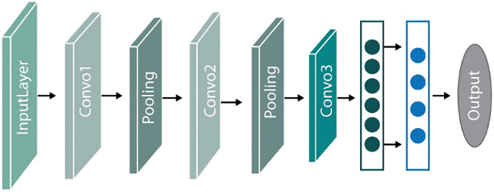
Figure 3: Overview of proposed CNN framework
In numerous, text and imaging classification approaches, CNN is considered efficient. In our proposed study, we utilized five convolutional layers CNN with pooling layers along with tuning of different hyperparameters and static vectors to attain excellent classification results. Our proposed architecture of CNN is shown in Fig. 4. This proposed CNN framework trains on a large feature vector illustration by passing the vector file through five convolutional filters and pooling layers. The main features of this proposed framework are the five connected convolutional layers along with the max-pooling layer to train a network that can distinguish microbleeds from non-microbleeds parts.
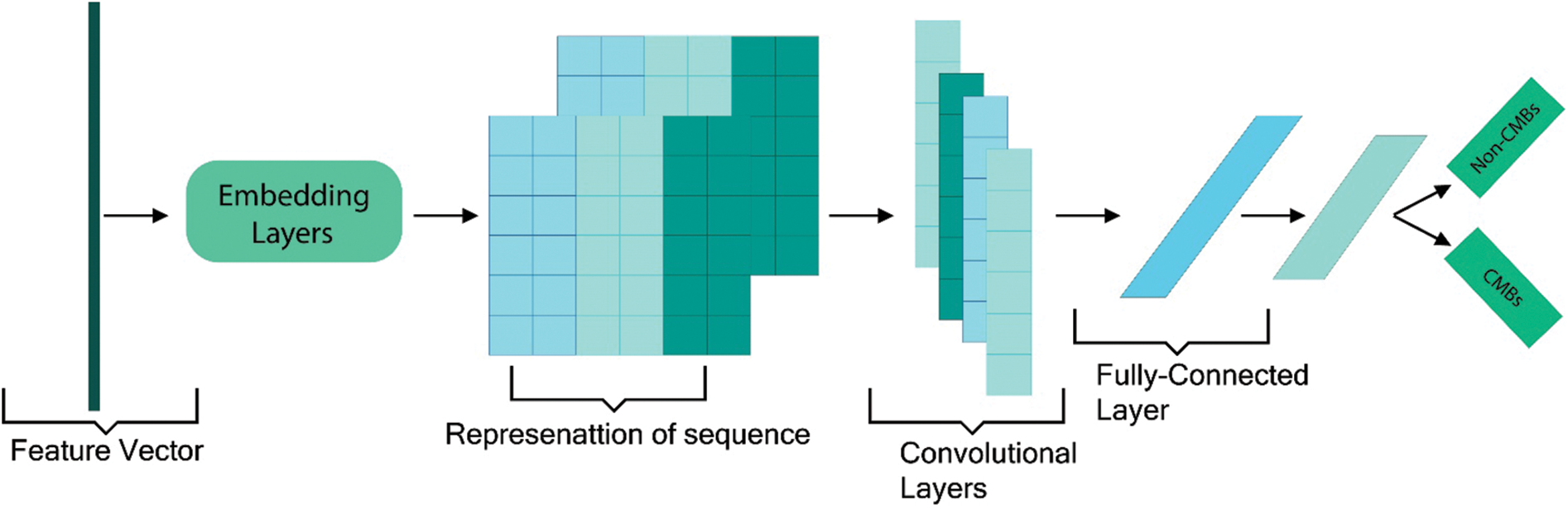
Figure 4: Proposed CNN framework with an example sentence
The first convolutio layers contain 96 numbers of kernels. The output get from this layer becomes the input of the second convolution layer having 256 kernels. Similarly, the next three convolution layers contain 384, 384, and 256 kernels, respectively. Unambiguously, the proposed framework implements a maximum pool approach to capture more and high fine-tuned features from the feature vector. A fully connected and softmax layers are added in between the last convolutional layer and output layer to get a more tuned feature vector. This decreases the dimension of the model as well as enhances the performance of the model. In the section, we explain our proposed study in detail. Suppose ei ∈ Rk is the vector in k dimensions relate to the i-th number of features of the vector file, (i = 1 to m), the entire vector file is characterized with the features concatenation e1:m = [e1…em] ∈ Rkm.
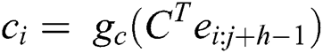
In general, the feature starting from i-th to j-th is characterized by e1:m = [e1…em] ∈ [Rk (j − i + 1)]. Convolutional layer C ∈ Rkh is used on features in which ci represents the convolutional non-linear function of activation, like ReLU functions. All the prejudiced terms are removed for conciseness and to keep simplicity. The ci altogether makes a featured map c = [c1,…, cm] ∈ Rm linked to the filter v that is applied. Multiple max-pooling filters are used along with five convolutional layers to get richer tuned and semantic data at the final output layer.
Let t be the number of parameters that are utilized and output feature maps are [c(1),…,c(t)]. A max pool process p(·) is used on each value of the feature map to generate a feature vector in dimension p, p(c(i)) ∈ Rp. The resultant output from the pooling layer goes to the next fully connected layers with h number of hidden points and with L units that are related to the values given to each label, symbolized by F ∈ RL in Eq. (6):

where Wh ∈ Rh × tp and Wo ∈ RL × h is weight-related to the final layer of CNN i.e., the output layer, and gh represents the activation function used in fully connected layers. In general, for classification purposes, a maximum pool layer is utilized. It means that take the maximum value from the whole feature map. This approach aims to take the maximum value, which means take values that have the highest number in each feature map. In this way, every time, the max pool will generate the highest single value, and the size of the final feature map is decreased this way. Furthermore, in our proposed approach, we utilized hyperparameters including the bias-learn-factor and learning-rate-factor to get optimal results and instead of generating only average values, we produce minimum, average, and maximum values and takes the maximum values to get more sophisticated features. This max-pooling method will generate better information per feature and send the larger rich information to the next connected layer. Fig. 5 illustrates the pooling example that how pooling filters can minimize the feature vector size.
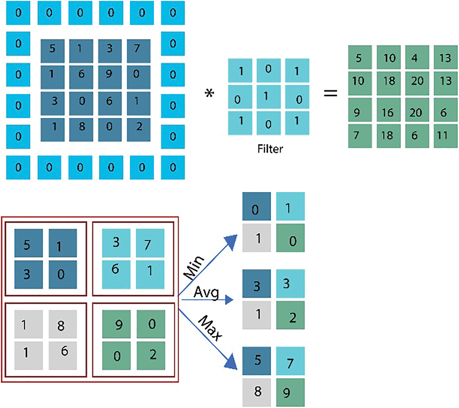
Figure 5: Graphical representation showing an example of feature vector selection using maximum pooling
The data samples utilized in this proposed study are SWI dataset of a total of 20 individuals for the identification of Cerebral Micro Bleeds (CMB). These data samples are the same percentage of the great size data set utilized in [23]. Many data samples have more than one cerebral in it. Fig. 6 shows a few examples where a single MRI contains more than one CMB. These MRI data samples are produced from a Philips-medical scheme of 3.0T by set the reiteration 17 ms in time, 512 × 512 × 150 in volume size, the reverberation time of 24 ms, in-plane goals of 0.45 × 0.45 mm, and cut thickness of 2 mm and cut separating of 1 mm. The entire dataset is marked by two experienced raters by following a micro-drain functional rating-scale [24].
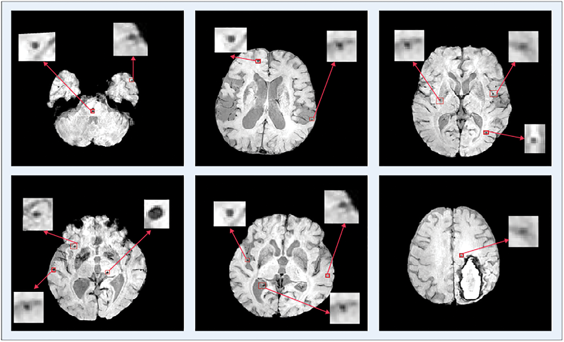
Figure 6: Single and multiple cerebral microbleeds in the brain MRI
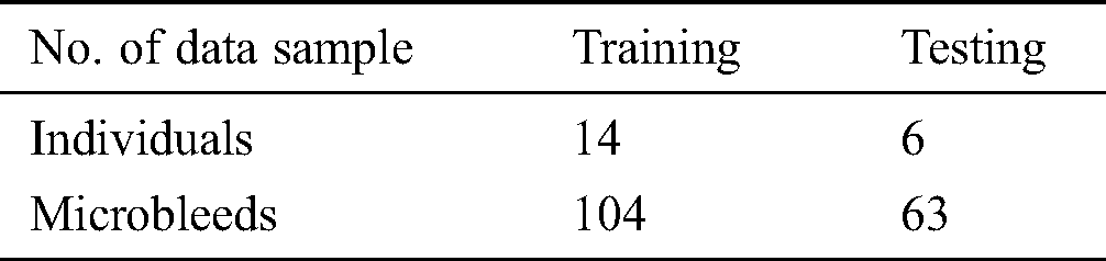
Now we have only used an axial perspective on 3D pictures. The data samples are separated into two parts, i.e., 20% of testing and 80% of training. The training samples use a total of 104 CMBs data samples from 14 individuals while 63 CMBs samples from 6 individuals have been utilized for testing. Tab. 2 shows data samples utilized in this study.
To assess the performance of our proposed framework, we use overall accuracy described as how neat the values, which are supposed to be measured, are to actual true values. Sensitivity is described as the calculated dimensions of true values that are true too. The specificity is described as calculated dimensions of false values that are predicted as false as well. The precision that is described as overall how accurate all measurements to the other measurements. These measures can be mathematically defined as:


where TP defines as the true positives that are also predicted as positive in output, TN defines as the true negative that is positive but predicted as negative in output. FP is defined as false positives that are negative but predicted as positive in output and FN is defined as false negatives that are positive but predicted as negative in output.
The data is split into an 80:20 ratio where 80% data are used for training and 20% was utilized for the testing purpose. Both the divisions have guaranteed to have both classes of CMBs and Non-CMBs. The proposed technique investigated a large feature-set to attain better performance. The primary purpose of the high false-positive rate in the detection of CMB is a highly intense and complex skull in MRI examines. The classification phase gets frequently confused and mixes the skull part with CMBs. For this reason, we removed the outer part of the skull from the brain MRI. Fig. 7 shows the graphical illustration, as well as the original skull, stripped brain image, in which the skull part was removed from the actual inner brain to reduce the error of false positives.
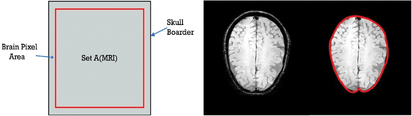
Figure 7: Removed skull part from the brain MRI
As discussed earlier, CMBs are minute particles having a tiny size and the trouble in detecting microbleeds is because of the presence of similar healthy cells. The k-mean clustering algorithm is also called hard clustering. This algorithm is simple and fast, but its limitation is that it cannot fragment CMBs very efficiently if it is malignant.
It depends on an iterative procedure that partitions the neuroimage into different clusters. The data points or the pixels are grouped in the best possible way such that if any specific data point has a place with a specific cluster. Fig. 8 shows some sample clusters generated by k-mean. We generate four different clusters from k-mean and select the best one with the region of interest and less false-positive values. It can be seen in Fig. 8 that cluster K2 has a very prominent region of interest and false positives are also less, therefore, we choose cluster 1.
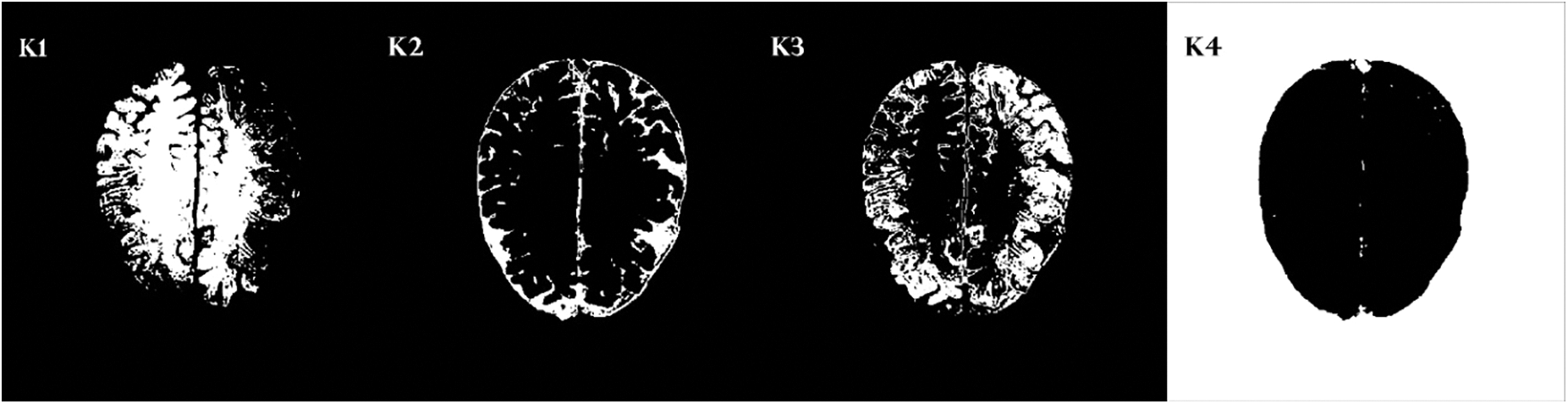
Figure 8: Four cluster samples generating by k-mean clustering
Furthermore, in detecting CMBs by utilizing a regular k-mean approach the desired results are difficult to achieve. We made changes in the traditional approach as it is not powerful enough for CMBs. We are required to design a more efficient algorithm that can handle this difficult problem without depending upon pre-processing and other steps. To get smooth and accurate detection if any non-micro bleed part is detected as CMBs, it will highly impact the overall classification of neuroimaging. Figs. 9 and 10 show the Non-CMBs and CMBs region in brain images, respectively.
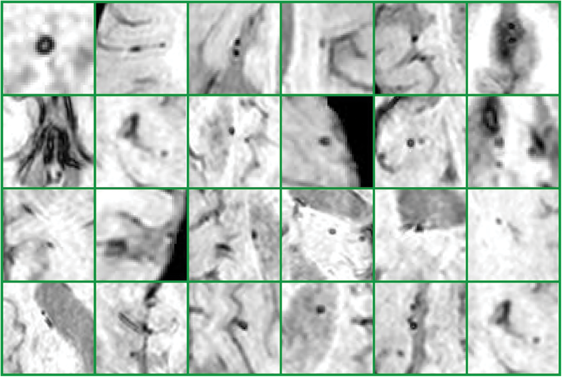
Figure 9: 6 × 4 = 24 samples of false classes of Non-CMBs particles
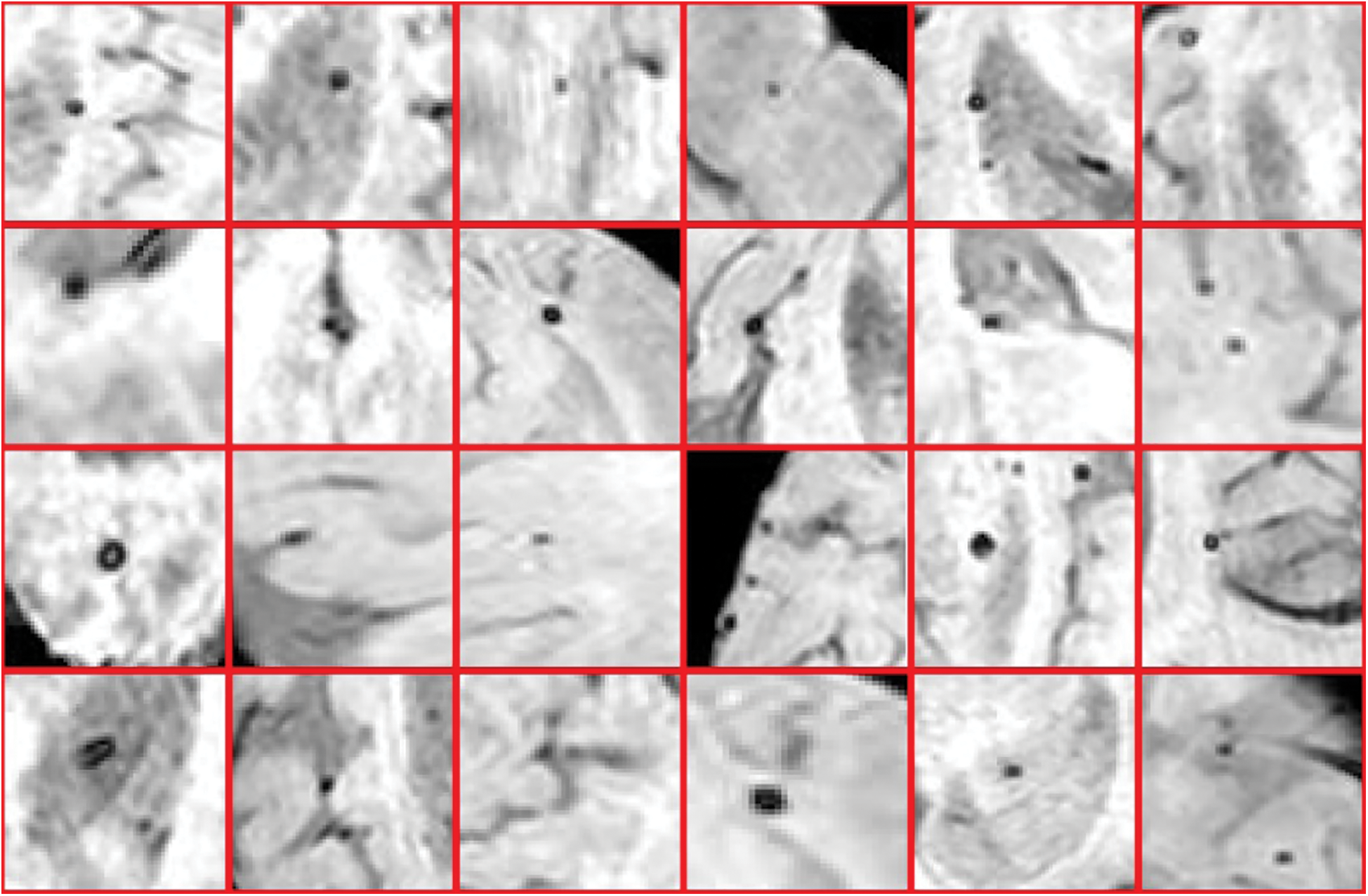
Figure 10: 4 × 6 = 24 samples of true classes having CMBs in brain MRI
Above all, the experiments were performed on Train_set of data samples which incorporates 14 individuals with CMBs. K-mean classifier is utilized for the subset in Train_set that had CMB to get 104 CMB from everyone in 14 individuals. At that point, some threshold values were used to get a region of interest arbitrarily from the sample’s size of MRI without CMB. After the ROI extraction process, only 334 ROIs were selected the extra particles were removed other than CMB based on size. Feature extraction is performed by considering 104 competitors and 334 non-bleeds. A Five-layer CNN framework is utilized for the characterization of the element vector.
After reducing the false positives from MRIs, statistical, Gaussian difference, Fourier transform, mean, median, variance, and geometrical based features were extracted from images. We applied a five-layer CNN model to classify the data samples into CMBs and Non-CMBs class. This proposed approach is assessed in the word of accuracy and precision. Tab. 3 shows the performance evaluation values utilizing a CNN of our proposed framework in terms of accuracy, precision, specificity, and sensitivity.
Table 3: Performance evaluation using CNN for the detection of CMBs
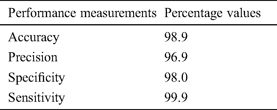
After extracting the features from ROIs in testing data, the resulted vector was then examined for classification through the CNN approach. In this experiment, we achieved 98.9% accuracy with 1 false-positive per CMB. We also generate a confusion matrix for all the training as well as testing data samples to observe the performance of the proposed study. We utilized the CNN approach with five convolutional layers and hyperparameters to discriminate microbleeds from non-micro bleeds. CMBs are so tiny in size and there may be more than 2 CMBs in one MRI. So, it is a challenging task to reduce false-positive and diagnose CMBs. To evaluate the performance of our proposed model, we compared the performance result of our model with state-of-art methods in terms of accuracy measure and sensitivity. To make a comparison method clear, we have used accuracy and sensitivity.
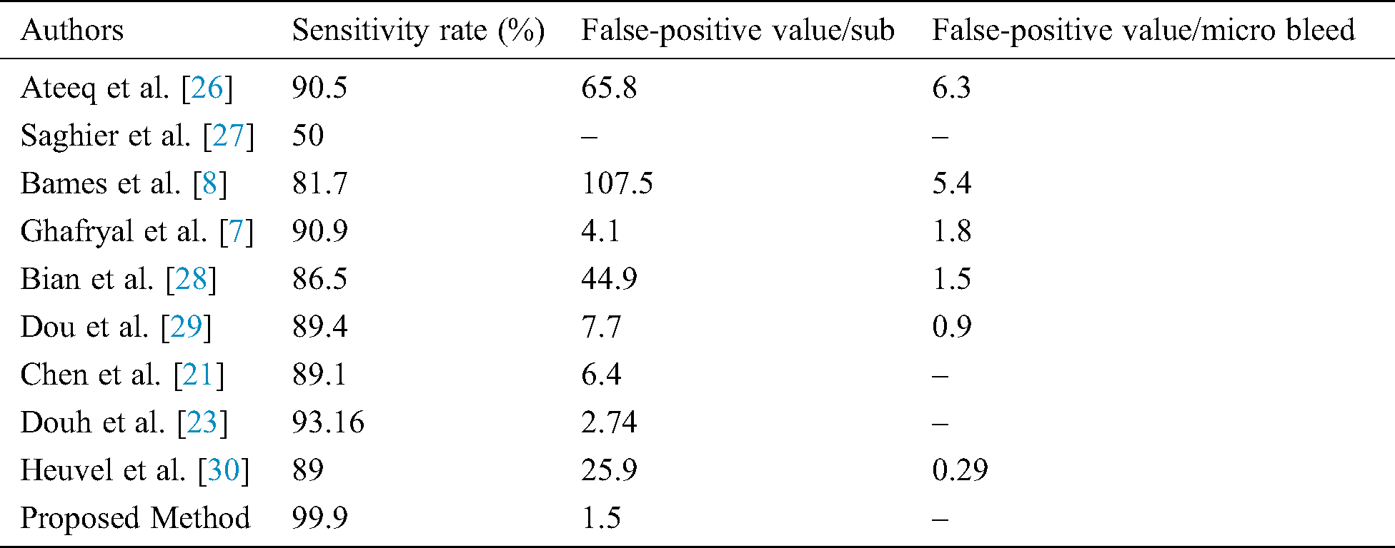
Different research groups Lu et al. [9], Hong et al. [10], Tao et al. [12], Wang et al. [25], and Ateeq et al. [26] utilized state of the art machine learning approaches to diagnose cerebral microbleeds from brain MRI. It can be seen from Tab. 4 that our proposed model achieved promising results in terms of performance accuracy and sensitivity. It is noticeable that the proposed study produces very good results in terms of false positives. It is worth mentioning here that most of the existing systems require a post-processing step to manually reduce false-positive rate. However, the proposed work is fully automated and there is no need to perform any post-processing step to reduce false-positive rate. As the proposed system requires no manual post-processing step for false-positive reduction, therefore, results are better or comparable to existing systems. The comparison should be made keeping in mind that our proposed system requires no post-processing step for false-positive reduction. Even then the performance of the proposed system is very good. Tab. 5 shows the comparison of false positives per individual as well as a comparison as per microbleeds.
Table 4: Comparison of the proposed model with state-of-the-art approaches in term of the accuracy measure
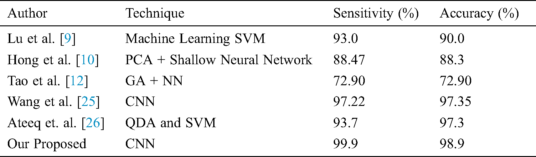
Table 5: Comparison of the proposed model with others in terms of false-positive values per subject and CMB
A Computer-Aided framework for characterizing ROIs is extensively useful for the diagnosis of CMBs. These frameworks can face a few impediments regarding affectability and false positives. The manual extraction of microbleeds is tough and takes a lot of time. Thus, the diagnosis of microbleeds and its classification from weighted images is still so challenging. The key objective of this proposed study to design an approach that is fully automated in reducing false positives and diagnosing CMB from the SWI images without any manual work. Another objective of this research is to enhance the performance accuracy of the system. The proposed work used CNN and clustering to reduce false positives. The proposed framework can recognize CMBs from non-CMB precisely, which gives a diagnosing reference to specialists. The proposed system handles a two-class binary classification issue. The performance accuracy, sensitivity, and specificity of the system are 98.9%, 99.9%, and 98% respectively. Concerning the future bearings of this work, CMBs identification can be additionally researched by utilizing further developed neural networks and transfer learning approaches. Additionally, the proposed framework can be improved by developing up a progressively complex feature extraction procedure.
Acknowledgement: The authors are grateful to the COMSATS University Islamabad, Attock Campus, Pakistan for their support for this research.
Funding Statement: This work was supported by the National Research Foundation of Korea (NRF) grant funded by the Korea government (MSIT) (NRF-2019R1F1A1058715).
Conflicts of Interest: The authors declare that they have no conflicts of interest to report regarding the present study.
1. S. M. Greenberg, M. W. Vernooij, C. Cordonnier, A. Viswanathan, R. A. S. Salman. (2009). et al., “Cerebral microbleeds: A guide to detection and interpretation,” Lancet Neurology, vol. 8, pp. 165–174. [Google Scholar]
2. Y. H. Fan, L. Zhang, W. W. Lam, V. C. Mok and K. S.Wong. (2003). “Cerebral microbleeds as a risk factor for subsequent intracerebral hemorrhages among patients with acute ischemic stroke,” Stroke, vol. 34, no. 10, pp. 2459–2462. [Google Scholar]
3. M. M. Poels, M. A. Ikram, A. Van der Lugt, A. Hofman, W. J. Niessen. (2012). et al., “Cerebral microbleeds are associated with worse cognitive function: The rotterdam scan study,” Neurology, vol. 78, pp. 326–333. [Google Scholar]
4. E. M. Haacke, S. Mittal, Z. Wu, J. Neelavalli and Y. C. Cheng. (2009). “Susceptibility-weighted imaging: Technical aspects and clinical applications, part 1,” American Journal of Neuroradiology, vol. 30, no. 1, pp. 19–30. [Google Scholar]
5. S. Liu, S. Buch, Y. Chen, H. S. Choi, Y. Dai. (2017). et al., “Susceptibility-weighted imaging: Current status and future directions,” NMR in Biomedicine, vol. 30, e3552. [Google Scholar]
6. H. J. Kuijf, J. De Bresser, G. J. Biessels, M. A. Viergever and K. L. Vincken. (2011). “Detecting cerebral microbleeds in 7.0 t mr images using the radial symmetry transform,” in IEEE Int. Sym. on Biomedical Imaging: From Nano to Macro, Chicago, Illinois, USA, pp. 758–761. [Google Scholar]
7. B. Ghafaryasl, F. Van der Lijn, M. Poels, H. Vrooman, M. A. Ikram. (2012). et al., “A computer aided detection system for cerebral microbleeds in brain MRI,” in 9th IEEE Int. Sym. on Biomedical Imaging, Barcelona, Spain, pp. 138–141. [Google Scholar]
8. P. P. Kim, B. W. Nasman, E. L. Kinne, U. E. Oyoyo, D. K. Kido. (2017). et al., “Cerebral microhemorrhage: A frequent magnetic resonance imaging finding in pediatric patients after cardiopulmonary bypass,” Journal of Clinical Imaging Science, vol. 7, pp. 1–5. [Google Scholar]
9. S. Lu, K. Xia and S. H. Wang. (2020). “Diagnosis of cerebral microbleed via VGG and extreme learning machine trained by gaussian map bat algorithm,” Journal of Ambient Intelligence and Humanized Computing, vol. 2014, no. 6, pp. 1–12. [Google Scholar]
10. J. Hong and Z. Lu. (2019). “Cerebral microbleeds detection via discrete wavelet transform and back propagation neural network,” in 2nd Int. Conf. on Social Science, Public Health and Education, Sanya, China. [Google Scholar]
11. W. Bian, C. P. Hess, S. M. Chang, S. J. Nelson and J. M. Lupo. (2013). “Computer-aided detection of radiation-induced cerebral microbleeds on susceptibility-weighted MR images,” NeuroImage: Clinical, vol. 2, pp. 282–290. [Google Scholar]
12. Y. Tao and R. S. Cloutie. (2018). “Voxelwise detection of cerebral microbleed in CADASIL patients by genetic algorithm and back propagation neural network,” in 3rd Int. Conf. on Communications, Information Management and Network Security, Wuhan, China. [Google Scholar]
13. H. N. Wang and B. Gagnon. (2017). “Cerebral microbleed detection by wavelet entropy and naive bayes classifier,” in 2nd Int. Conf. on Biomedical and Biological Engineering, Guilin, China. [Google Scholar]
14. S. Roy, A. Jog, E. Magrath, J. A. Butman and D. L. Pham. (2015). “Cerebral microbleed segmentation from susceptibility weighted images,” Medical Imaging 2015: Image Processing, vol. 9413, 94131E. [Google Scholar]
15. Y. D. Zhang, Y. Zhang, X. X. Hou, H. Chen and S. H. Wang. (2018). “Seven-layer deep neural network based on sparse autoencoder for voxelwise detection of cerebral microbleed,” Multimedia Tools and Applications, vol. 77, no. 9, pp. 10521–10538. [Google Scholar]
16. A. Fazlollahi, F. Meriaudeau, V. L. Villemagne, C. C. Rowe, P. Yates. (2014). et al., “Efficient machine learning framework for computer-aided detection of cerebral microbleeds using the radon transform,” in IEEE 11th Int. Sym. on Biomedical Imaging, pp. 113–116. [Google Scholar]
17. T. Van den Heuvel, A. Van Der Eerden, R. Manniesing, M. Ghafoorian, T. Tan. (2016). et al., “Automated detection of cerebral microbleeds in patients with traumatic brain injury,” NeuroImage: Clinical, vol. 12, pp. 241–251. [Google Scholar]
18. S. R. Barnes, E. M. Haacke, M. Ayaz, A. S. Boikov and W. Kirsch. (2011). “Semiautomated detection of cerebral microbleeds in magnetic resonance images,” Magnetic Resonance Imaging, vol. 29, pp. 844–852. [Google Scholar]
19. K. He, X. Zhang, S. Ren and J. Sun. (2016). “Deep residual learning for image recognition,” in Proc. of the IEEE Conf. on Computer Vision and Pattern Recognition, Las Vegas, Nevada, United States, pp. 770–778. [Google Scholar]
20. Q. Dou, H. Chen, L. Yu, L. Zhao, J. Qin. (2016). et al., “Automatic detection of cerebral microbleeds from MR images via 3D convolutional neural networks,” IEEE Transactions on Medical Imaging, vol. 35, pp. 1182–1195. [Google Scholar]
21. H. Chen, L. Yu, Q. Dou, L. Shi and V. C. Mok. (2015). “Automatic detection of cerebral microbleeds via deep learning based 3d feature representation,” in IEEE 12th Int. Sym. on Biomedical Imaging, New York, USA, pp. 764–767. [Google Scholar]
22. K. He, X. Zhang, S. Ren and J. Sun. (2016). “Identity mappings in deep residual networks,” in European Conf. on Computer Vision, Amsterdam, The Netherlands, pp. 630–645. [Google Scholar]
23. S. P. Singh, L. Wang, S. Gupta, H. Goli, P. Padmanabhan. (2004). et al., “3D deep learning on medical images: A review,” arXiv Preprint, arXiv:2004.00218, vol. 20, pp. 1–14. [Google Scholar]
24. S. M. Gregoire, H. Jäger, T. A. Yousry, C. Kallis, M. M. Brown. (2010). et al., “Brain microbleeds as a potential risk factor for antiplatelet-related intracerebral haemorrhage: Hospital-based, case-control study,” Journal of Neurology, Neurosurgery & Psychiatry, vol. 81, no. 6, pp. 679–684. [Google Scholar]
25. S. Wang, J. Sun, I. Mehmood, C. Pan and Y. Chen. (2020). “Cerebral micro-bleeding identification based on a nine-layer convolutional neural network with stochastic pooling,” Concurrency and Computation: Practice and Experience, vol. 32, pp. e5130. [Google Scholar]
26. T. Ateeq, M. N. Majeed, S. M. Anwar, M. Maqsood, Z. U. Rehman. (2018). et al., “Ensemble-classifiers-assisted detection of cerebral microbleeds in brain MRI,” Computers & Electrical Engineering, vol. 69, pp. 768–781. [Google Scholar]
27. M. L. Seghier, M. A. Kolanko, A. P. Leff, H. R. Jäger and S. M. Gregoire. (2011). “Microbleed detection using automated segmentation (MIDASA new method applicable to standard clinical MR images,” PLoS One, vol. 6, pp. 1–9. [Google Scholar]
28. X. Zou, B. L. Hart, M. Mabray, M. R. Bartlett and W. Bian. (2017). “Automated algorithm for counting microbleeds in patients with familial cerebral cavernous malformations,” Neuroradiology, vol. 59, pp. 685–690. [Google Scholar]
29. Q. Dou, H. Chen, L. Yu, L. Shi and D. Wang. (2015). “Automatic cerebral microbleeds detection from MR images via independent subspace analysis based hierarchical features,” in 37th Annual Int. Conf. of the IEEE Engineering in Medicine and Biology Society, Milan, Italy, pp. 7933–7936. [Google Scholar]
30. F. S. Feltrin, A. L. Zaninotto, V. M. P. Guirado, F. Macruz and D. Sakuno. (2018). “Longitudinal changes in brain volumetry and cognitive functions after moderate and severe diffuse axonal injury,” Brain Injury, vol. 32, pp. 1413–1422. [Google Scholar]
 | This work is licensed under a Creative Commons Attribution 4.0 International License, which permits unrestricted use, distribution, and reproduction in any medium, provided the original work is properly cited. |