Deep Learning in DXA Image Segmentation

Dildar Hussain; Rizwan Naqvi; Woong-Kee Loh; Jooyoung Lee

doi:10.32604/cmc.2021.013031

1School of Computational Science, Korea Institute for Advanced Study (KIAS), 85 Hoegiro, Dongdaemun-gu, Seoul, 02455, South Korea
2Department of Unmanned Vehicle Engineering, Sejong University, 209, Neungdong-ro, Gwangjin-gu, Seoul, 05006, South Korea
3Department of Software, Gachon University, Seongnam, 13120, South Korea
*Corresponding Author: Jooyoung Lee. Email: jlee@kias.re.kr
Received: 22 July 2020; Accepted: 26 August 2020

Abstract: Many existing techniques to acquire dual-energy X-ray absorptiometry (DXA) images are unable to accurately distinguish between bone and soft tissue. For the most part, this failure stems from bone shape variability, noise and low contrast in DXA images, inconsistent X-ray beam penetration producing shadowing effects, and person-to-person variations. This work explores the feasibility of using state-of-the-art deep learning semantic segmentation models, fully convolutional networks (FCNs), SegNet, and U-Net to distinguish femur bone from soft tissue. We investigated the performance of deep learning algorithms with reference to some of our previously applied conventional image segmentation techniques (i.e., a decision-tree-based method using a pixel label decision tree [PLDT] and another method using Otsu’s thresholding) for femur DXA images, and we measured accuracy based on the average Jaccard index, sensitivity, and specificity. Deep learning models using SegNet, U-Net, and an FCN achieved average segmentation accuracies of 95.8%, 95.1%, and 97.6%, respectively, compared to PLDT (91.4%) and Otsu’s thresholding (72.6%). Thus we conclude that an FCN outperforms other deep learning and conventional techniques when segmenting femur bone from soft tissue in DXA images. Accurate femur segmentation improves bone mineral density computation, which in turn enhances the diagnosing of osteoporosis.

Keywords: Segmentation; deep learning; osteoporosis; dual-energy X-ray absorptiometry

Osteoporosis, as a severe degrader of bone health and the leading cause of hip fracture in developed countries, leaves a grave burden on health budgets. The repercussions of this disease are noted to be the same among women and men and can affect them at any stage of life. More than 20% of people die from fractures that occur from osteoporosis [1]. The medical imaging technology known as dual-energy X-ray absorptiometry (DXA) can adequately diagnose this disease and is currently considered the gold standard for such diagnoses [2–4]. Meanwhile, quantitative computed tomography exists as an alternative method, but it demands a large dose of X-rays and is overpriced.

Reliable osteoporosis analysis is dependent on accurate computation of bone mineral density (BMD). Careful DXA image analysis and precise BMD calculation support the pinpoint segmentation of soft tissue and bone. On the other hand, imprecise bone and soft tissue segmentation severely affect BMD calculation and subsequent analysis of DXA image [3,4]. Unfortunately, erroneous bone region identification is a widespread problem in femur DXA images for several reasons. First, DXA images use low-dose X-rays, which makes them prone to noise. Second, the overlap of the hip muscles and pelvic bone over the femur head generates different intensities for the various regions and the femur in the image. Third, the irregular attenuation of an X-ray through the human body creates a negative shadow, which causes gloomy regions in the images. Other factors influencing segmentation characteristics include luminous intensity, scanning orientation, person-to-person variations, and image resolution [5].

Regardless of the numerous techniques that have been used so far, accurate automatic segmentation in DXA imaging remains a challenge [6–13]. Manual segmentation is time-consuming, requiring the involvement of an expert, and such an approach is untenable when it comes to analyzing a fairly large population [7,9,10]. Edge-detection-based image segmentation methods are unreliable due to hurdles in the final integration of tiny boundaries to find broad object edges in an image [7]. The calibration procedure for specific DXA imaging devices and the diversity present in DXA data make it challenging to specify an acceptable threshold value in threshold-based segmentation techniques, again creating a less-than-ideal situation for segmentation in DXA imaging [7,8]. Active appearance models or active shape models are often used in DXA image segmentation as well [11,13]. The convergence of landmark points with an active shape model determines the ultimate location of an object. However, the active shape model sometimes converges on inaccurate boundaries for an object due to variations between patients. It is often challenging to describe the Mahalanobis distance in an active shape model with a sparse covariance matrix. Meanwhile, an active appearance model uses a Gaussian space to match an object’s shape through a statistical model. But assumptions made with Gaussian space matching often fail due to bone structure variations, particularly in patients with osteophytes [14]. The abovementioned techniques demand close initialization of the model to a segmentation subject. Furthermore, the structural specification ambivalence produced by the partial-volume effect makes other segmentation techniques, such as region growing, unsuitable for femur segmentation in DXA imaging [15]. Segmentation of X-ray images using a watershed algorithm habitually results in over-segmentation [16]. Because of all the intrinsic constraints associated with current methods, they are inappropriate for the segmentation of DXA images. Thus, there remains a desperate need to find a self-activating DXA image segmentation approach that grants higher accuracy.

In recent years, the term deep learning has been widely used in the analysis of biological and biomedical images, such as those dealing with the detection of cancerous and mitosis cells, skin lesion classification, neural membrane segmentation, immune cell detection, the segmentation of masses in mammograms, and so on [17–26]. The development of deep convolutional neural networks (CNNs) and recent maturation in their use has led to fully convolutional networks (FCNs) [27] being effectively used for nodule detection and segmentation in biomedical imaging systems such as computed tomography and magnetic resonance images [28–32]. Despite the possible use of deep learning for image inspection in other medical imaging systems, it has not been applied to DXA imaging.

In this work, our purpose is to research the feasibility of deep learning approaches for accurate segmentation in DXA imaging. We introduce and investigate the performance of the most up-to-date and novel deep learning approaches for a multiclass pixel-wise semantic model, such as one using SegNet, U-Net, or an FCN, for femur segmentation from DXA images. To the best of our knowledge, this is the first deep-learning-based effort relevant to DXA image segmentation. We compare the results of this study to one of our previous works on femur segmentation from DXA images using a machine-learning-based approach called pixel label decision tree, which was reported in [33] and published by the Journal of X-Ray Science and Technology.

We conducted a detailed investigation to figure out the capability of recent deep CNN approaches for femur segmentation from DXA images. The best results were achieved with a deep FCN-based architecture. This technique takes advantage of the fact that a DXA scan produces low-energy (LE) and high-energy (HE) images that are then merged to create high-contrast images. Various algorithms can be used with the combinations of HE and LE images to generate high-contrast results [33–37]. These DXA images are saved as portable network graphic files.

The main intention of this study is to identify a highly accurate solution for femur segmentation from DXA images. Improved DXA image segmentation will support accurate BMD calculation, and better BMD calculation can strengthen the diagnosing capability of DXA machines. Besides that, improved automatic DXA image segmentation will increase the use of DXA imaging devices. Through this study, we show how convolutional networks can be trained from end to end, pixel to pixel, with a small clinical dataset using transfer learning in semantic segmentation. Our key insight is to introduce a convolutional network with efficient inference and learning on a small sample of DXA data.

The rest of the manuscript is ordered as follows. Section 2 covers the segmentation model. Section 3 shows the proposed model’s results and includes a discussion of the findings. Finally, Section 4 presents our concluding remarks and possibilities for future work.

Femur data are attained from DXA scanning as LE and HE images. The X-ray images are captured by the receptor and maintained in digital records for further processing. These two images undergo a process that yields high-contrast electronic display images.

In medical image processing and computer vision, recent techniques based on deep neural networks have accomplished state-of-the-art and impressive outcomes on large-scale datasets with millions of images belonging to different categories. Regarding their impressive achievements, deep neural networks have been shown to be susceptible to image quality [38]. Thus, image quality is an important consideration in these approaches. Improving the visual quality of an image through measures such as contrast enhancement and noise reduction has had an impressive effect on image classification and segmentation [39,40]. We acquired DXA data in the form of LE and HE images and combined them to form high-contrast display images. In this study, we consider a high-contrast bone mineral density image (BMDI) generated from a DXA scan and its effect on deep learning segmentation results. These high-contrast BMDIs can be generated from DXA scans as follows:

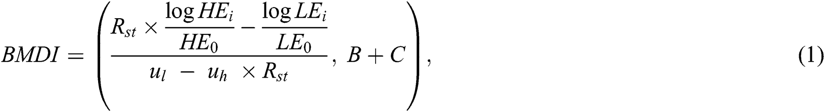
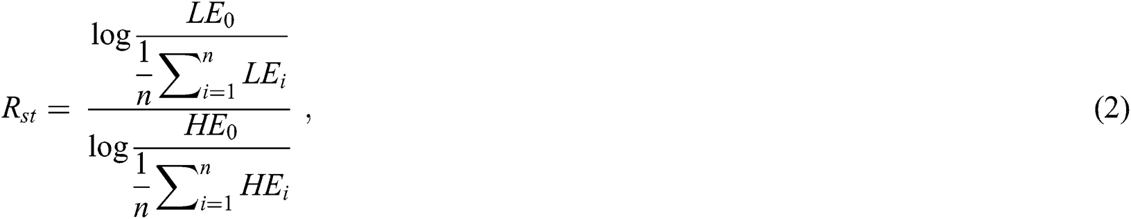
where ul and uh are constant values of LE and HE X-rays, respectively. The incident HE0 and LE0 are the outcome energies from the X-ray s source, and LEi and HEi are detector counts at a particular scanning position (i.e., the image pixel). The BMD value for the soft tissue region is always lower than the bone region; therefore, Eq. (1) produces a brighter bone and darker soft tissue image. The Rst value (as shown in Eq. (2) is calculated first and then used to generate the BMDI in Eq. (1). Similarly, C and B depict image contrast enhancement and brightness. We used C and B as constant values preserved from the experiments. We normalized the intensities of an image from 0 to 255, and the final image was extracted as a portable network graphic file to be used in the deep learning model.

A huge dataset is required to appropriately train deep learning networks. The small-scale availability of medical datasets is one of the most challenging dilemmas in a deep learning approach. In order to meet the large dataset requirements of deep neural network training, a small data size can be increased using data augmentation [41,42]. This is the most familiar and comfortable method to reduce deep neural network overfitting problems.

Therefore, in this study, we applied the data augmentation process only to the training data (i.e., 80% of the 900 images) as follows. We randomly selected a set of femur images from the training dataset (i.e., 80% of the 900 images) and applied image translations and horizontal and vertical reflections along with labeled ground truth images to increase the data size. We extracted random 192 × 96 patches from 384 × 192 images and applied horizontal flip, vertical flip, and their subsequent scaling to 384 × 192 using linear interpolation. The augmentation process increased the size of our available dataset up to 2,500 images. The translation process produced a black pixel gap in an image that was filled with an air class. Thus, a total of 2,000 femur images with their correlate ground truth labels were used to train our suggested segmentation methods.

Furthermore, we followed the transfer learning idea to intensify the training competence of our proposed deep learning models. We employed the weights of the pre-trained model Visual Geometry Group 16 network using the immense ImageNet dataset [17]. Then we fine-tuned our prepared networks using the augmented training data. A separate validation dataset (i.e., 20% of the original training dataset) was used to optimize the proposed segmentation models. All the femur images were resized to 384 × 192 pixels using bilinear interpolation [13].

An overview of DXA image analysis using deep learning methods is given in Fig. 1. In this study, we present U-Net, SegNet, and FCN methods to segment femur in a DXA image. The FCNs estimate a dense return from an arbitrary-sized feed in data. In this manner, both “learning and inference are carried out on the entire image at a time by dense feedforward computation and backpropagation” [43]. The CNN-based deep learning models are usually found with fully-connected layers. The name fully convolutional in the FCN model points to convolutional layers without any fully connected layers in the model. We have used a sigmoid activation function in the activation layer of the suggested deep learning segmentation networks to classify each pixel in the femur image into three classes (i.e., bone, soft tissue, and air). More details about the U-Net, SegNet, and FCN techniques are given in [43–45]. The Adadelta optimization method was used to train all the segmentation models with a batch size of 25. The initial learning rate was set as 0.2, which was reduced during the training process with automatic updates throughout 200 epochs.

Figure 1: Overview of dual energy X-ray absorptiometry image analysis using deep learning

We used weighted cross-entropy to calculate the loss, which minimized the overall loss, H, throughout the training stage as follows:

where

is the ground truth labels and images

represents the predicted map of segmentation. C represents the class. M is the number of classes (bone, tissue, and air). The implementation of this work was performed with Python on the Ubuntu 18.04 operating system using the Keras library with the Theano backend.

No post-processing was performed for the deep learning models. Contrasted to deep learning models, conventional semantics segmentation techniques always require a boundary smoothing filter to smooth femur bone boundaries labeled by the segmentation model and remove imperfections. In our previous study, we used a binary smoothing filter to remove such imperfections from the segmented DXA images. “Binary smoothing removes small-scale noise in the shape while maintaining large-scale features. For more details about binary smoothing, visit our previous work referenced in” [33].

The difference between model-based prediction and ground truth annotations was noted by the number of TN (true negatives), TP (true positives), FN (false negatives), and FP (false positives), where n is the total number of observations such that n = TN + TP + FN + FP. The accuracy of each model was calculated according to the following procedures.

The Jaccard index (JI) or intersection over union (IOU) is the estimated reliability of the segmented object with ground truths.

where “TP is the object area (correctly classified) common between segmented image and ground truth. FP and FN are the numbers of bone and soft tissue pixels wrongly classified between two classes (bone and soft tissue)” [33].

Sensitivity, “also known as the positive prediction rate (TPR), measures the proportion of positive pixels identified accurately” [33]. “In a sensitivity test, the number of correctly classified bone tissue pixels in the femur DXA image is compared to the ground truth” [33]:

where “TP is the total number of correctly classified pixels representing bone, and GTb is the ground truth in bone pixels” [33].

Specificity, “also known as the true-negative prediction rate (TNR), measures the proportion of negative pixels accurately identified” [33]. “In a specificity test, the number of correctly classified soft tissue pixels in a femur DXA image is compared to ground truth” [33]:

where “TN is the total number of pixels correctly classified as soft tissue and GTt is the ground truth in rejection of the bone pixels” [33].

The false-positive prediction rate (FPR) is the measure of soft tissue pixels wrongly classified as bone:

Meanwhile, the false-negative prediction rate (FNR) is the measure of bone pixels wrongly classified as soft tissue:

“The test performance of each method per image was calculated by comparing the segmentation output of a femur object to the ground truth” [33]. “We used sensitivity, specificity, and IOU tests to measure the accuracy of an individual image” [33]. “A segmentation method was considered to have failed to segment a femur object in a test image correctly if IOU < 0.92, sensitivity < 95%, or specificity < 93%” [33]. “The final accuracy of the model was calculated by comparing the number of accurately segmented images out of the total number of test images” [33]:

In the above equation, JI is the Jaccard index, φ is the image segmentation sensitivity, and υ is the image segmentation specificity. The 2,500 (original + augmented) DXA images were divided for experiments as follows: 60% were used for training, 20% were used for validation to optimize the parameters of all the segmentation models, and remaining 20% were used for independent testing.

Previously, we used some conventional techniques (i.e., Otsu’s thresholding and a pixel label decision tree) to segment femur in DXA images using handcrafted features. Thus, we compared the results of the current deep-learning-based segmentation to our previous work. For more details, visit our previous work referenced in [33].

We used the same dataset from our previous study titled “Femur Segmentation in DXA Imaging Using a Machine Learning Decision Tree” [33], with some additional femur images acquired from a DXA scanner (OsteoPro MAX, YOZMA B.M. Tech Co., Ltd., Republic of Korea). Radiology experts manually segmented femur images as the ground truth. Manual annotations were extracted from the DXA system in the portable network graphic file format along with high-contrast images to train and test our deep learning models. Each and every pixel in a femur image was annotated and assigned a class label (i.e., either bone, soft tissue, or air).

This section presents the performance of the U-Net, SegNet, and FCN approaches using the test data (i.e., 500 femur images). Tab. 1 shows the segmentation performance results in terms of average accuracy computed using the JI, sensitivity, and specificity of all the test images. Some output examples of the segmented femur DXA images are shown in Fig. 2 using different segmentation methods. A couple of the predicted segmentation contours based on the different segmentation models are shown in Fig. 3.

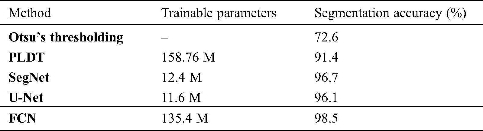
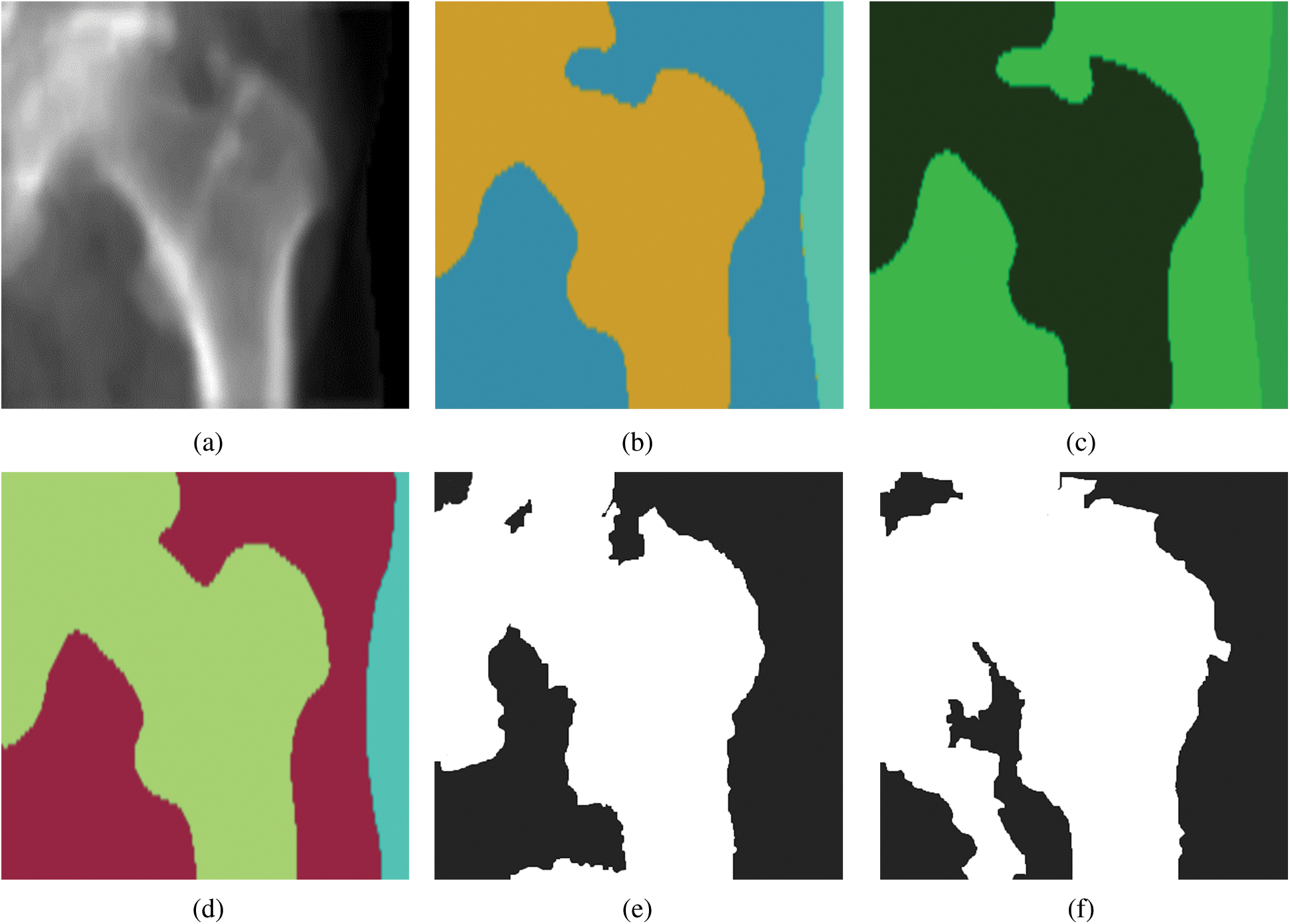
Figure 2: Dual energy X-ray absorptiometry image segmentation with different models: (a) a femur image, (b) a femur image segmented by SegNet, (c) a femur image segmented by U-Net, (d) a femur image segmented by a fully convolutional network, (e) a femur image segmented by a pixel label decision tree, and (f) a femur image segmented by Otsu’s thresholding

Segmenting femur images with significantly higher accuracy (i.e., 98.5%) occurred from using an FCN in comparison to the other segmentation models. Optimal results were produced with an FCN when it was fine-tuned to the DXA data. We segmented 500 test femur images with an FCN and other deep learning models. Each model demonstrated soaring performance over the conventional models in high-contrast femur sections (the femur head and shaft), as well as in most challenging areas (e.g., the greater and lesser trochanters). Data were collected on multiple devices, and the models covered the diversity of the data and were robust.

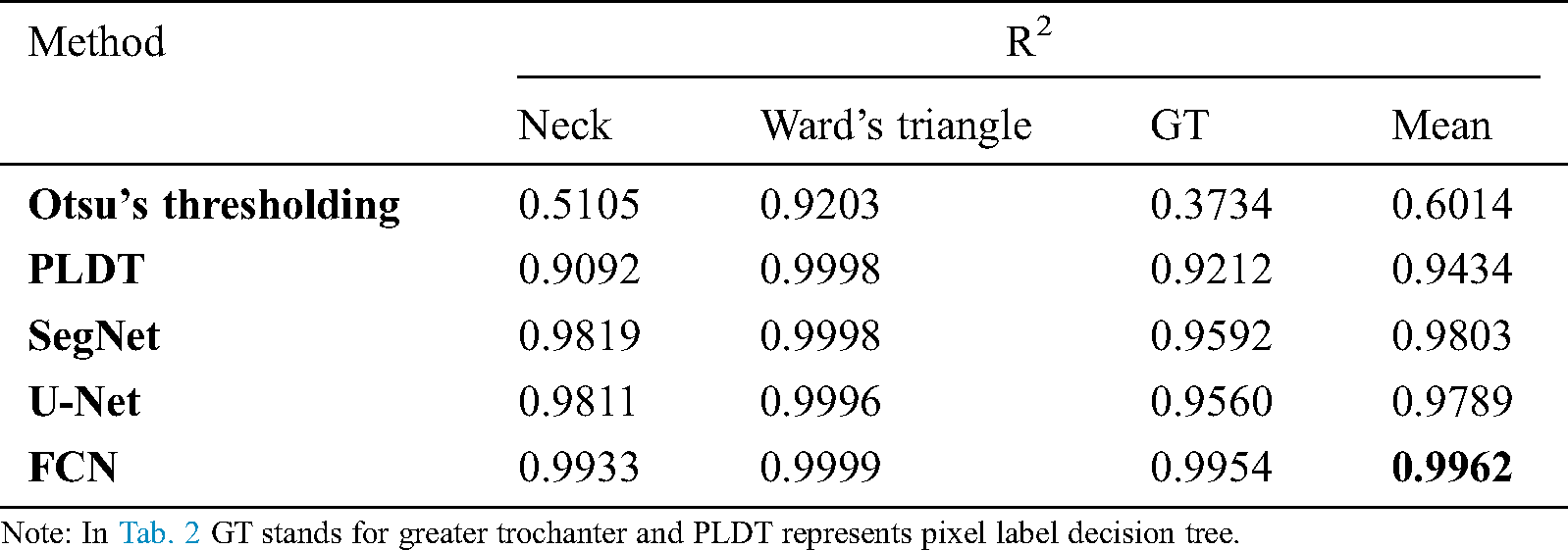
We performed a BMD consistency check on model-segmented images in comparison to manually segmented ones. First, we randomly selected 100 femur images and gave them to three persons to manually segment the femur, select regions of interest, and calculate the BMD at three different regions, that is, the femur neck, Ward’s triangle, and the greater trochanter. Second, an average value was recorded from three expert readings at the three femur regions (i.e., the femur neck, Ward’s triangle, and the greater trochanter) for each instance of the image. Then the estimations were compared with the model-based segmentation to check the consistency of each model. Finally, we carried out a statistical correlation study (by calculating the coefficient of determination, R2) of the BMD measurements between the different segmentation methods and manual segmentation. The FCN segmentation method scored the highest correlation record as shown in Tab. 2.

Figure 3: Predicted femur boundaries with SegNet, U-Net, and a fully convolutional network. The red contours represent ground truths, the yellow contours represent SegNet, the blue contours represent U-Net, and the green contours represent the fully convolutional network

The results demonstrate that the FCN method yields higher sensitivity, specificity, and accuracy than the other models. The FCN model provides a practical and powerful technique for the segmentation issue in DXA imaging. Although a CNN model is considered an innovative and genuine segmentation method, it requires an extensive amount of training data. We followed the transfer learning idea to raise the training capability of deep learning models on a small number of femur DXA images. We employed the weights of the pre-trained model Visual Geometry Group16 network by using the immense ImageNet dataset. Our previous study presented on femur segmentation [33] shows that current deep learning models performed better than previously applied models.

A conventional problem for deep learning is the fact that it is hard to train a CNN-based network with limited data without using optimized techniques and data augmentation. For this reason, appropriate optimization methods, data augmentation, and transfer learning can assist in training a reliable segmentation network. Transfer learning fine-tunes the deep network that has been pre-trained on medical or general images. Set side by side with data augmentation, transfer learning is an additional distinct solution with many parameters. To address this issue, we successfully implemented the transfer learning solution with DXA images that had already been segmented with another solution (i.e., those from ImageNet).

During the correlation analysis of femur BMD measurement, we found a significantly higher correlation (R2 = 0.962) between the measurement from an FCN-segmented femur images compared to the expert-segmented ones. Further investigations may be able to identify the serviceability of FCN and other deep learning models in the clinical diagnosis of osteoporosis and the prediction of fracture risk. All deep-learning-based models were shown to perform better than previously applied techniques. The study has demonstrated that convolutional networks can be effectively used with a high level of performance on a small clinical dataset through transfer learning in semantic segmentation.

We presented a deep-learning-based technique for femur segmentation in DXA imaging and focused on improving segmentation accuracy. The predictive performance and efficiency of an FCN on femur data was stunning. The practical use of the FCN method in DXA image segmentation has the potential to enhance the validity of BMD analysis and clinical diagnosis of osteoporosis.

Our results demonstrate that the FCN model can be used for DXA image segmentation since it performs well on femur DXA images with proper tuning of the model. One limitation of the deep learning approach is that these models suffer from poor generalization when the input data comes from different DXA machines (due to different acquisition parametrization, system models, system calibration, etc.). Our next research step will focus on this issue.

Acknowledgement: Special thanks to YOZMA B.M. Tech Co., Ltd., Republic of Korea, and its employees for providing data for this research.

Funding Statement: This research was supported by Basic Science Research Program through the National Research Foundation of Korea (NRF) funded by the Ministry of Science and ICT [NRF-2017R1E1A1A01077717].

Conflicts of Interest: The authors declare that they have no conflicts of interest to report regarding the present study.

References

K. M. Karlsson, I. Sernbo, K. J. Obrant, I. R. Johnell and O. Johnell. (1996). “Femur neck geometry and radiographic signs of osteoporosis as predictors of hip fracture,” Bone, vol. 18, no. 4, pp. 327–330.
K. A. John. (2002). “Diagnosis of osteoporosis and assessment of fracture risk,” Lancet, vol. 359, no. 9321, pp. 1929–1936.
R. Dendere, J. H. Potgieter, S. Steiner, S. P. Whiley and T. S. Douglas. (2015). “Dual-energy X-ray absorptiometry for measurement of phalangeal bone mineral density on a slot-scanning digital radiography system,” IEEE Transactions on Biomedical Engineering, vol. 62, no. 12, pp. 2850–2859.
N. F. A. Peel, A. Johnson, N. A. Barrington, T. W. D. Smith and D. R. Eastell. (1993). “Impact of anomalous vertebral segmentation on measurements of bone mineral density,” Journal of Bone and Mineral Research, vol. 8, no. 6, pp. 719–723.
F. Ding, W. K. Leow and T. Howe. (2007). “Automatic segmentation of Femur bones in anterior-posterior pelvis X-ray images,” in Int. Conf. on Computer Analysis of Images and Patterns, Berlin, Heidelberg: Springer, pp. 205–212.
C. S. CriŞan and S. Holban. (2013). “A comparison of X-ray image segmentation techniques,” Advances in Electrical and Computer Engineering, vol. 13, no. 3, pp. 85–92.
K. E. Naylor, E. V. McCloskey, R. Eastell and L. Yang. (2013). “Use of DXA-based finite element analysis of the proximal Femur in a longitudinal study of hip fracture,” Journal of Bone and Mineral Research, vol. 28, no. 5, pp. 1014–1021.
T. A. Burkhart, K. L. Arthurs and D. M. Andrews. (2009). “Manual segmentation of DXA scan images results in reliable upper and lower extremity soft and rigid tissue mass estimates,” Journal of Biomechanics, vol. 42, no. 8, pp. 1138–1142.
H. Yasufumi, Y. Kichizo, F. M. I. Toshinobu, T. Kichiya and N. Yasuho. (1990). “Assessment of bone mass by image analysis of metacarpal bone roentgenograms: A quantitative digital image processing (DIP) method,” Radiation Medicine, vol. 8, no. 5, pp. 173–178.
C. Matsumoto, K. Kushida, K. Yamazaki, K. Imose and T. Inoue. (1994). “Metacarpal bone mass in normal and osteoporotic Japanese women using computed X-ray densitometry,” Calcified Tissue International, vol. 55, no. 5, pp. 324–329.
J. P. Wilson, K. Mulligan, B. Fan, J. L. Sherman, E. J. Murphy et al.. (2012). , “Dual-energy X-ray absorptiometry-based body volume measurement for 4-compartment body composition,” The American Journal of Clinical Nutrition, vol. 95, no. 1, pp. 25–31.
12. M. Roberts, T. Cootes, E. Pacheco and J. Adams. (2007). “Quantitative vertebral fracture detection on DXA images using shape and appearance models,” Academic Radiology, vol. 14, no. 10, pp. 1166–1178.
N. Sarkalkan, H. Weinans and A. A. Zadpoor. (2014). “Statistical shape and appearance models of bones,” Bone, vol. 60, pp. 129–140.
J. Wu and M. R. Mahfouz. (2016). “Robust X-ray image segmentation by spectral clustering and active shape model,” Journal of Medical Imaging, vol. 3, no. 3, 034005.
D. L. Pham, C. Xu and J. L. Prince. (2000). “Current methods in medical image segmentation,” Annual Review of Biomedical Engineering, vol. 2, no. 1, pp. 315–337.
L. Siyuan, S. Wang and Y. Zhang. (2017). “A note on the marker-based watershed method for X-ray image segmentation,” Computer Methods and Programs in Biomedicine, vol. 141, pp. 1–2.
D. Ciresan, A. Giusti, L. M. Gambardella and J. Schmidhuber, “Mitosis detection in breast cancer histology images with deep neural networks,” in Medical Image Computing and Computer Assisted Interventions (MICCAI 2013), Springer, Berlin, Heidelberg, pp. 411–418, 2013.
18. C. Malon and E. Cosatto. (2013). “Classification of mitotic figures with convolutional neural networks and seeded blob features,” Journal of Pathology Informatics, vol. 4, no. 1, pp. 9.
19. A. Cruz-Roa, A. Basavanhally, F. Gonzalez, H. Gilmore, M. Feldman et al. (2014). , “Automatic detection of invasive ductal carcinoma in whole slide images with convolutional neural networks,” SPIE Medical Imaging, vol. 9041, 904103.
20. A. Cruz-Roa, J. Arevalo, A. Madabhushi and F. Osorio. (2013). “A deep learning architecture for image representation visual interpretability and automated basal-cell carcinoma cancer detection,” in Medical Image Computing and Computer-Assisted Intervention (MICCA 2013), vol. (LNCS, 8150),pp. 403–410.
21. D. Ciresan, A. Giusti, L. Gambardella and J. Schmidhuber, “Deep neural networks segment neuronal membranes in electron microscopy images,” in Proc. of the 25th Int. Conf. on Neural Information Processing Systems (NIPS 2012), Curran Associates Inc., 57 Morehouse Lane, Red Hook, NY, USA, vol. 2, pp. 2843–2851, 2012.
22. T. J. Brinker, A. Hekler, J. S. Utikal, N. Grabe, D. Schadendorf et al., “Skin cancer classification using convolutional neural networks: systematic review,” Journal of Medical Internet Research, vol. 20, no. 10, pp. 1–8, 2018.
23. T. Chen and C. Chefdhotel. (2014). “Deep learning based automatic immune cell detection for immunohistochemistry images, ” in 5th Int. Workshop on Machine Learning in Medical Imaging (MLMI’14), Boston, MA, USA,pp. 17– 24.
24. N. Dhungel, G. Carneiro and A. P. Bradley, “Deep learning and structured prediction for the segmentation of mass in mammograms,” in Medical Image Computing and Computer Assisted Intervention (MICCAI 2015), Springer, Cham, Munich, Germany, pp. 605–612, 2015.
25. N. Dhungel, G. Carneiro and A. P. Bradley. (2014). “Deep structured learning for mass segmentation from mammograms,” . [online]. Available: http://arxiv.org/abs/.
X. L. Yang, S. Y. Yeo, J. M. Hong, S. T. Wong, W. T. Tang et al., “A deep learning approach for tumor tissue image classification,” in Proc. of Biomedical Engineering, Innsbruck, Austria, ACTA Press, pp. 1–7, 2016.
J. Long, E. Shelhamer and T. Darrell, “Fully convolutional networks for semantic segmentation,” in Proc. of the IEEE Conf. on Computer Vision and Pattern Recognition, Boston, Massachusetts, pp. 3431–3440, 2015.
B. A. Skourt, E. I. Abdelhamid and A. Majda. (2018). “Lung CT image segmentation using deep neural networks,” Procedia Computer Science, vol. 127, pp. 109–113.
29. Y. Jia, E. Shelhamer, J. Donahue, S. Karayev, J. Long et al., “Caffe: Convolutional architecture for fast feature embedding,” in Proc. of the 22nd ACM Int. Conf. on Multimedia, Orlando, Florida, USA, ACM, pp. 675–678, 2014.
30. H. C. Shin, H. R. Roth, M. Gao, L. Lu, Z. Xu et al. (2016). , “Deep convolutional neural networks for computer-aided detection: CNN architectures, dataset characteristics and transfer learning,” IEEE Transactions on Medical Imaging, vol. 35, no. 5, pp. 1285–1298.
31. X. Yang, Z. Zeng and S. Yi. (2017). “Deep convolutional neural networks for automatic segmentation of left ventricle cavity from cardiac magnetic resonance images,” IET Computer Vision, vol. 11, no. 8, pp. 643–649.
P. V. Tran. (2016). “A fully convolutional neural network for cardiac segmentation in short-axis MRI,” Computer Vision and Pattern Recognition, . arXiv preprint arXiv: 1604. 00494. https://arxiv.org/abs/1604,
D. Hussain, M. A. Al-antari, M. A. Al-masni, S. M. Han and T. S. Kim. (2018). “Femur segmentation in DXA imaging using a machine learning decision tree,” Journal of X-ray Science and Technology, vol. 26, no. 5, pp. 727–746.
34. M. A. Al-antari, M. A. Al-masni, M. Metwallyb, D. Hussain, S. J. Parkb et al. (2018). , “Denoising images of dual energy X-ray absorptiometry using non-local means filters,” Journal of X-ray Science and Technology, vol. 26, no. 3, pp. 395–412.
35. M. A. Al-Antari, M. A. Al-Masni, M. Metwally, D. Hussain, E. Valarezo et al., “Non-local means filter denoising for DXA images,” in 2017 39th Annual Int. Conf. of the IEEE Engineering in Medicine and Biology Society (EMBC), Jeju Island, S. Korea, pp. 572–575, 2017.
36. D. Hussain, S. M. Han and T. S. Kim. (2019). “Automatic hip geometric feature extraction in DXA imaging using regional random forest,” Journal of X-ray Science and Technology, vol. 27, no. 2, pp. 207–236.
D. Hussain and S. M. Han. (2019). “Computer-aided osteoporosis detection from DXA imaging,” Computer Methods and Programs in Biomedicine, vol. 173, pp. 87–107.
S. Dodge and L. Karam, “Understanding how image quality affects deep neural networks,” in IEEE, 2016 Eighth Int. Conf. on Quality of Multimedia Experience (QoMEX), Lisbon, Portugal, pp. 1–6, 2016.
S. Calderon, F. Fallas, M. Zumbado, P. N. Tyrrell, H.Stark et al. (2018). , “Assessing the impact of the deceived non-local means filter as a preprocessing stage in a convolutional neural network based approach for age estimation using digital hand x-Ray images,” in 2018 25th IEEE Int. Conf. on Image Processing (ICIP) IEEE, pp. 1752–1756.
G. B. P. da Costa ,W. A. Contato, T. S. Nazare, J. E. S. B. Neto and M. Ponti, “An empirical study on the effects of different types of noise in image classification tasks,” Computer Vision and Pattern Recognition, pp. 1–6, 2016.
S. Kaur, R. Hooda, A. Mittal and S. Sofat. (2017). “Deep CNN-based method for segmenting lung fields in digital chest radiographs,” in Advanced Informatics for Computing Research. Singapore: Springer, pp.185–194.
A. Krizhevsky, I. Sutskever and G. E. Hinton, “Imagenet classification with deep convolutional neural networks,” in Advances in Neural Information Processing Systems, Harrahs and Harveys, Lake Tahoe, NeurIPS, pp. 1097–1105, 2012.
E. Shelhamer, J. Long and T. Darrell. (2017). “Fully convolutional networks for semantic segmentation,” IEEE Transactions on Pattern Analysis and Machine Intelligence, vol. 39, no. 4, pp. 640–651.
44. O. Ronneberger, P. Fischer and T. Brox, “U-net: Convolutional networks for biomedical image segmentation,” in Int. Conf. on Medical Image Computing and Computer-Assisted Intervention, Munich, Germany, pp. 234–241, 2015.
V. Badrinarayanan, A. Kendall and R. Cipolla. (2017). “Segnet: A deep convolutional encoder-decoder architecture for image segmentation,” IEEE Transactions on Pattern Analysis and Machine Intelligence, vol. 39, no. 12, pp. 2481–2495.

Computers, Materials & Continua DOI:10.32604/cmc.2021.013031
Article