DOI:10.32604/cmc.2021.012666

| Computers, Materials & Continua DOI:10.32604/cmc.2021.012666 |  |
| Article |
Numerical Study of Computer Virus Reaction Diffusion Epidemic Model
1Department of Computer Science, The University of Lahore, Lahore, Pakistan
2Department of Mathematics, Cankaya University, Ankara, Turkey
3Institute of Space Sciences, Magurele-Bucharest, Romania
4Department of Medical Research, China Medical University Hospital, China Medical University, Taichung, Taiwan
5Department of Mathematics and Statistics, The University of Lahore, Lahore, Pakistan
6Department of Mathematics, National College of Business Administration and Economics Lahore, Lahore, Pakistan
7Faculty of Engineering, University of Central Punjab, Lahore, Pakistan
8Department of Mathematics, University of Management and Technology, Lahore, Pakistan
*Corresponding Author: Ali Raza. Email: Alimustasamcheema@gmail.com
Received: 14 July 2020; Accepted: 16 July 2020
Abstract: Reaction–diffusion systems are mathematical models which link to several physical phenomena. The most common is the change in space and time of the meditation of one or more materials. Reaction–diffusion modeling is a substantial role in the modeling of computer propagation like infectious diseases. We investigated the transmission dynamics of the computer virus in which connected to each other through network globally. The current study devoted to the structure-preserving analysis of the computer propagation model. This manuscript is devoted to finding the numerical investigation of the reaction–diffusion computer virus epidemic model with the help of a reliable technique. The designed technique is finite difference scheme which sustains the important physical behavior of continuous model like the positivity of the dependent variables, the stability of the equilibria. The theoretical analysis of the proposed method like the positivity of the approximation, stability, and consistency is discussed in detail. A numerical example of simulations yields the authentication of the theoretical results of the designed technique.
Keywords: Computer virus dynamics; reaction–diffusion system; positive solution; simulations
Computer viruses are automated programs that, against the users’ wish, make copies of themselves to spread to new targets and as a result infect the computers [1]. With the accelerated advancement of modern technologies, the internet has assimilated into each part of our life, which is a great help for us, as well as it also poses a serious problem to individual and corporate computer systems through cyber-attacks [2]. A lot of effort has been dedicated to studying how to avoid harmful actions. To control effectively the diffusion of computer viruses, it is very crucial to figure out the ways that nasty codes propagate over the Internet. In order to minimize the threat of virus spread, various strategies can be proposed by using epidemic models. In 2018, Ali et al. [3] studied the Padé approximation method to describe the propagation of a computer virus via the SEIR model. Due to the compelling analogy between a computer virus and a biological virus, some classic computer virus epidemic models, such as SIRS, SIS, SIR, SLB, SEIR, delayed, and stochastic models were proposed and studied. In epidemics, the most common fatal infectious diseases are measles, malaria, HIV/AIDS, tuberculosis, influenza, etc., determine the individual mechanisms and environmental conditions that have contributed to their spread. Epidemic modeling helps to identify the specific areas of virus spread and also predict effective preventives and creative measures to control it [4]. Mishra et al. [5] presented various mathematical models on computer viruses. In 2017, Kumar [6] developed a SIRA dynamical model of the computer virus. In 2008, Doud et al. [7] proposed computer virus plans and discovery methods by using different delays. In 2015, Ebenezer et al. [8] presented the SIER mathematical model by the use of local and global sense dynamics of computer bugs productivity. In 2019, Ozdemir et al. [9] proposed the SEIR-KS model of fractional order model for computer virus transmission. In 2015, Oztürk et al. [10] presented the mathematical modeling of an improved version of the SIR model. Rey [11] investigated the dynamics of computer virus spread in the system of networks. In 2019, Lanz et al. [12] proposed the SEI1I2QR model in which they examine types of malware acquired based on infection symptoms treatment. In 2016, Xu et al. [13] presented the SEIR model to discuss the spread of malware in the presence of anti-virus capacity. In 2016, Liu et al. [14] represented the SIQR model by utilizing two delays strategy. In 2008, Yuan et al. [15] described the SEIR model by use of three crucial networking environmental factors. In 2012, Yang et al. [16] suggested the SLBS model in which explains the prohibition of malware on the internet. In 2020, Dubey et al. [17] studied the analytically schemes for malware spread through the network and proposed the CVP model. In 2020, Arif et al. [18] investigated the stochastic dynamics of the computer propagation model by using the different numerical techniques in which focus on the structure-preserving method. In our opinion, the epidemic models for computer viruses can help to better understanding how the viruses diffuse on networks. In this study, we extend a computer virus epidemic model by placing a diffusion term. We determine the conditions under which epidemics are likely to occur. The computer virus has a latent period, during which individuals are exposed to a computer virus but are not yet infectious. An infected computer which is in latency, will not infect other computers immediately; however, it still can be infected [19]. In this study, the following reaction–diffusion computer virus epidemic model is proposed for numerical analysis which is an extended form of the model given by Persaei et al. [20].


with initial conditions
 ,
,  ,
,  ,
,
and homogenous Neumann boundary conditions. Where  represents the class of uninfected computers,
  represents latent computers and
  represents the seizing computers at time
 . The constant rate of connecting external computers with internet and disconnecting internal computers from internet is denoted by
  is the constant rate of infection and the term
  is the percentage of internal computers infected at time t.
  is the constant rate of latent computer breakout. Latent computers are cured at the constant rate of
  , while breaking out computers are cured at the constant rate of
  .
.  are constant rate of diffusion. All these parameters used in this model are positive. It is observed that the variables of interest of the proposed computer virus model are the computer populations. Now it is the basic need for the solution of system (Eqs. (1)–(3)) to be positive as values of unknown variables involved are taken as absolute [21]. In the present era, several positivity persevering numerical techniques are proposed by various authors because many dynamical continuous systems require the positive solution [22,23]. The current work is dedicated to designing and analyzing a finite difference algorithm which retains the positive solution of the state variables of the continuous system for the solution of computer virus epidemic model (Eqs. (1)–(3)). This manuscript is sectioned as follows. The reproductive number and equilibrium points of the system under study is explained in Section 2. In Section 3, a numerical algorithm is designed to solve the computer virus epidemic system. In the same section, the theoretical analysis of the proposed technique is performed. It is shown that the designed numerical technique is capable of retaining the positivity of the solution. The stability and consistency of the proposed algorithm are also authenticated in this section. Section 4 is devoted to the computation results. The simulations are justified the theoretical results of the designed method.
The model Eqs. (1)–(3) admits two equilibrium points, VFE (virus free equilibrium)  , and the CVE (computer virus endemic equilibrium point)
where, 

 and reproductive number of the model is
Divide  into
into  with step sizes
  and
and . Grid points are


 ,
,  and
and  are denoted as finite difference approximations of
  and
and  respectively.
Take Eq. (1)


Similarly we have from Eq. (2) and Eq. (3) simultaneously.


where  and
and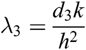 .
.
3.1 Consistency of the Proposed Scheme
This section is concerned about the verification of the proposed scheme to be consistent. For this,


By putting all these definitions’ in Eq. (7), we have


Similarly we can check for  and
and  i.e.,
i.e.,


Hence our proposed scheme is consistent and first order accurate in time and second order accurate in space.
3.2 Stability of Proposed Scheme
In this section, we will use von Neumann stability criteria to show our proposed implicit scheme from Eqs. (4)–(6) is unconditionally stable. For this purpose, we will introduce the following terms,
 ,
,  ,
, 
And 
Put all these terms in Eq. (4), we have

where 

After proper calculation and rearranging terms, we have

Take absolute value on both sides, we have the following inequality,

By using similar process for Eq. (5), and Eq. (6) simultaneously we have, we have

and

Inequalities from Eqs. (11)–(13) are showing that our proposed implicit scheme is unconditionally stable by using von Neumann stability analysis.
Theorem 1: For any positive  and
and  ,
,  and
and  appertaining the to the Eqs. (4)–(6) are positive for all
Proof: We will use m-matrix theory and mathematical induction to show our scheme preserve positivity. For this purpose rewrite Eqs. (4)–(6) in vector form, as


If  represents any of
  or
or  where these are all real square matrices, then
  can be written in general form as

The off-diagonal and diagonal entries of  are
are  ,
,  and
and  . The off-diagonal and diagonal entries of
  are
are  ,
,  and
and  . The off-diagonal and diagonal entries of
  are
are  ,
,  and
and  .
.
Thus  are m-matrices.
This implies  are non-singular matrices. So Eqs. (14)–(16) can be written as


Suppose that  ⇒
⇒  and
and 
Also  are m-matrices. This guarantees that all the entries of
  are positive. The product of two positive matrices is also positive.
⇒ R.H.S of Eqs. (17)–(19) are 
So  are also positive.
Hence our proposed implicit scheme preserve positivity.
4 Numerical Example and Simulations
In this section, we demonstrate a numerical example and simulations for the application of proposed structure preserving technique. For this we consider the following initial conditions,


First we discuss the simulations of proposed structure preserving method at CVF point. For the CVF point we take the following values of parameters involved in the model so that the value of  is less than one.
 ,
,  ,
,  ,
,  ,
,  ,
,  ,
,  ,
, 
Figs. 1–3 demonstrate the numerical solution of model by implementing the proposed technique at the VFE point. It is given that the VFE point of the computer virus model is  . This point is stable when the reproductive number values are less than one. So it is concluded that the computer virus epidemic model under study possesses two main properties, positive solution, and stability of both equilibria. It is evident from Figs. 1–3 that the simulation results are with the good agreement of theorem 1. The proposed structure-preserving technique retains positive solutions and stability of the CVF point. The graphs of susceptible, latent, and breaking out computers shows the convergence towards VFE point
  .
.
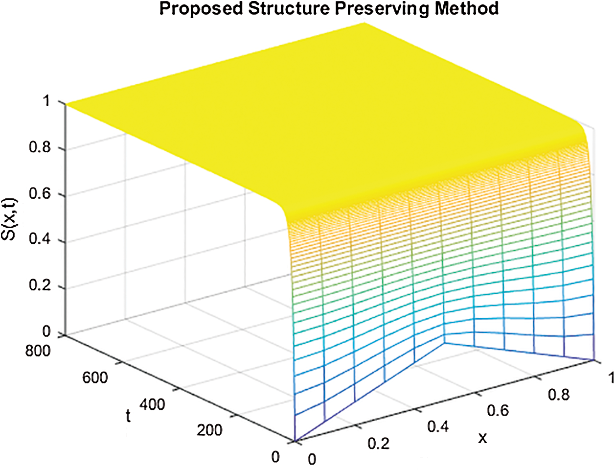
Figure 1: The solution graphs of susceptible computers representing the behavior of proposed structure preserving technique with values of step sizes  and
and 
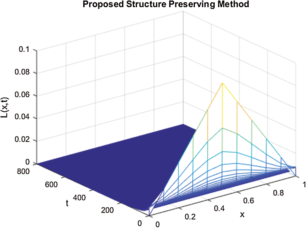
Figure 2: The solution graphs of latent computers representing the behavior of proposed structure preserving technique with values of step sizes  and
and 
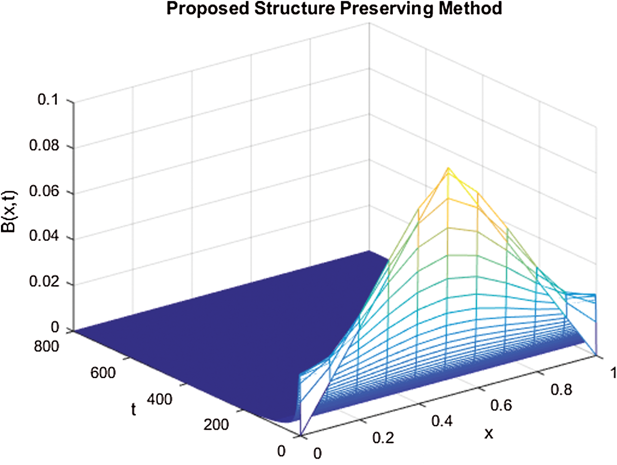
Figure 3: The solution graphs of breaking out computers representing the behavior of proposed structure preserving technique with values of step sizes  and
and 
Now we present the simulations of proposed structure preserving method at CVE point. For the CVE point we use the following values of parameters involved in the model so that the value of  is greater than one.
  ,
,  ,
,  ,
,  ,
,  ,
,  ,
,  ,
, 
Figs. 4–6 describe the graphical solution of the system by using the proposed technique at CVE point. The CVE point is stable when the reproductive number values are greater than one. It is clearly shown from the Figs. 4–6 that the proposed structure-preserving numerical technique sustains the positive behavior of the solution of continuous system. Also, this method preserves the stability of the CVF point. It is validated from the solution graphs of susceptible, latent and breaking out computers in above figures as the sketches in these figures show the convergence towards CVE point  .
.
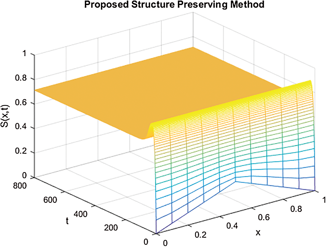
Figure 4: The solution graphs of susceptible computers representing the behavior of proposed structure preserving technique with values of step sizes  and
and 

Figure 5: The solution graphs of latent computers representing the behavior of proposed structure preserving technique with values of step sizes  and
and 
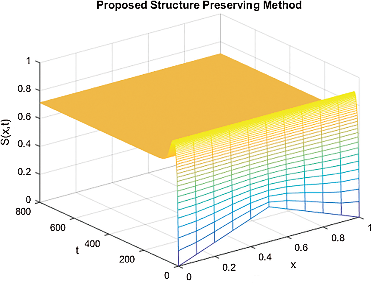
Figure 6: The solution graphs of breaking out computers representing the behavior of proposed structure preserving technique with values of step sizes  and
and 
In this paper, we propose an extended reaction–diffusion epidemic model of computer virus dynamics for the numerical investigation. An efficient and reliable numerical technique is designed which preserves the stability of equilibria and positivity of the approximation. The stability, consistency, and positivity of the proposed algorithm are shown mathematically and are validated graphically with the help of a numerical example. The proposed algorithm can be used for the solution of reaction–diffusion models like predator-prey models, chemical reaction models and infectious disease models. In future work, we shall extend the modeling of a computer virus in the computer population in the well-known notations like fractional and stochastic fractional-order derivatives [24–26].
Acknowledgement: The authors are grateful to anonymous referees. Also, thankful to the Vice-Chancellor of University of the Lahore, National College of Business Administration and Economics Lahore and University of Central Punjab Lahore, for providing an excellent research environment and facilities.
Funding Statement: The authors declare that they have no funding for the present study.
Conflicts of Interest: The authors declare that they have no conflicts of interest to report regarding the present study.
1. A. Raza, M. S. Arif, M. Rafiq, M. Bibi, M. Naveed et al.. (2019). , “Numerical treatment for stochastic computer virus model,” Computer Modeling in Engineering and Sciences, vol. 120, no. 2, pp. 445–465. [Google Scholar]
2. L. Yang and X. Yang. (2014). “A new epidemic model of computer viruses,” Communications in Nonlinear Science and Numerical Simulation, vol. 19, no. 6, pp. 1935–1944. [Google Scholar]
3. J. Ali, M. Saeed, M. Rafiq and S. Iqbal. (2018). “Iqbal Numerical treatment of nonlinear model of virus propagation in computer networks: An innovative evolutionary padé approximation scheme,” Advances in Difference Equations, vol. 18, no. 01, pp. 214–228. [Google Scholar]
4. J. Li and P. Knickerbocker. (2007). “Functional similarities between computer worms and biological pathogens,” Computers and Security, vol. 26, no. 4, pp. 338–347. [Google Scholar]
5. B. K. Mishra and D. Saini. (2007). “Mathematical models on computer viruses,” Applied Mathematics and Computation, vol. 187, no. 2, pp. 929–936. [Google Scholar]
6. U. Kumar. (2016). “A dynamic model on computer virus,” Recent Advances in Mathematics Statistics and Computer Science, vol. 2, no. 1, pp. 504–510. [Google Scholar]
7. E. A. Doud, I. H. Jebril and B. Zaqaibeh. (2008). “Computer virus strategies and detection method,” International Journal of Open Problems in Computer Science and Mathematics, vol. 1, no. 2, pp. 1–18. [Google Scholar]
8. B. Ebenezer, N. Farai and A. S. Kwesi. (2015). “Fractional dynamics of computer virus propagation,” Science Journal of Aplied Mathematics and Statistics, vol. 3, no. 3, pp. 63–69. [Google Scholar]
9. N. Ozdemir, S. Uçar and B. B. I. Eroglu. (2019). “Dynamical analysis of fractional order model for computer virus propagation with kill signals,” International Journal of Nonlinear Sciences and Numerical Simulation, vol. 21, no. 3, pp. 239–247. [Google Scholar]
10. Y. Oztürk and M. Gulsu. (2015). “Numerical solution of a modified epidemiological model for computer viruses,” Applied Mathematical Modelling, vol. 39, no. 24, pp. 7600–7610. [Google Scholar]
11. A. M. D. Rey. (2015). “Mathematical modeling of the propagation of malware: A review,” Security and Communication Networks, vol. 8, no. 15, pp. 2561–2579. [Google Scholar]
12. A. Lanz, D. Rogers and T. L. Alford. (2019). “An epidemic model of malware virus with quarantine,” Journal of Advances in Mathematics and Computer Science, vol. 33, no. 4, pp. 1–10. [Google Scholar]
13. Y. H. Xu, J. G. Ren and G. Q. Sun. (2016). “Propagation effect of a virus outbreak on a network with limited anti-virus ability,” PLoS One, vol. 11, no. 10, pp. 1–18. [Google Scholar]
14. J. Liu, C. Bianca and L. Guerrini. (2016). “Dynamical analysis of a computer virus model with delays,” Discrete Dynamics in Nature and Society, vol. 16, no. 1, pp. 1–19. [Google Scholar]
15. H. Yuan and G. Chen. (2008). “Network virus-epidemic model with the point-to-group information propagation,” Applied Mathematics and Computation, vol. 206, no. 1, pp. 357–367. [Google Scholar]
16. X. Yang and L. Yang. (2012). “Towards the epidemiological modeling of computer viruses,” Discrete Dynamics in Nature and Society, vol. 12, no. 1, pp. 1–20. [Google Scholar]
17. V. P. Dubey, R. Kumar and D. Kumar. (2020). “A hybrid analytical scheme for the numerical computation of time fractional computer virus propagation model and its stability analysis,” Chaos Solutions & Fractals, vol. 133, no. 1, pp. 109–118. [Google Scholar]
18. M. Shoaib Arif, A. Raza, M. Rafiq, M. Bibi, J. Nawaz Abbasi et al.. (2020). , “Numerical simulations for stochastic computer virus propagation model,” Computers Materials and Continua, vol. 62, no. 1, pp. 61–77. [Google Scholar]
19. L. Yang, X. Yang, Q. Zhu and L. Wen. (2013). “A computer virus model with graded cure rates,” Nonlinear Analysis: Real World Applications, vol. 14, no. 1, pp. 414–422. [Google Scholar]
20. M. R. Parsaei, R. Javidan, N. S. Kargar and H. S. Nik. (2017). “On the global stability of an epidemic model of computer viruses,” Theory in Biosciences, vol. 136, no. 3–4, pp. 169–178. [Google Scholar]
21. B. M. C. Charpentier and H. V. Kojouharov. (2013). “An unconditionally positivity preserving scheme for advection diffusion reaction equations,” Mathematical and Computer Modelling, vol. 57, no. 9–10, pp. 2177–2185. [Google Scholar]
22. N. Ahmed, M. J. Jawaz, M. A. Rehman and M. Rafiq. (2018). “Numerical treatment of an epidemic model with spatial diffusion,” Journal of Applied Environmental and Biological Sciences, vol. 8, no. 6, pp. 17–29. [Google Scholar]
23. M. S. Arif, A. Raza, W. Shatanawi, M. Rafiq and M. Bibi. (2019). “A stochastic numerical analysis for computer virus model with vertical transmission over the Internet,” Computers Materials and Continua, vol. 61, no. 3, pp. 1025–1043. [Google Scholar]
24. E. K. Akgul. (2019). “Solutions of the linear and nonlinear differential equations within the generalized fractional derivatives,” Chaos: An Interdisciplinary Journal of Nonlinear Science, vol. 29, no. 2, pp. 1–19. [Google Scholar]
25. D. Baleanu, A. Fernandez and A. Akgul. (2020). “On a fractional operator combining proportional and classical differintegrals,” Mathematics, vol. 8, no. 3, pp. 1–13.
26. A. Atangana and A. Akgul. (2019). “Can transfer function and bode diagram be obtained from Sumudu transform,” Alexinderia Engineering Journal, vol. 1, no. 2, pp. 1–14. [Google Scholar]
 | This work is licensed under a Creative Commons Attribution 4.0 International License, which permits unrestricted use, distribution, and reproduction in any medium, provided the original work is properly cited. |