DOI:10.32604/cmc.2021.012469
| Computers, Materials & Continua DOI:10.32604/cmc.2021.012469 | |
| Article |
Motion-Based Activities Monitoring through Biometric Sensors Using Genetic Algorithm
1Department of Information Technology, College of Computer and Information Sciences, Majmaah University, Majmaah, 11952, Saudi Arabia
2ASET, Amity University Noida, Noida, 201301, India
3Computer Science Department, Community College, King Saud University, Riyadh, Saudi Arabia
*Corresponding Author: Mohammed Alshehri. Email: ma.alshheri@mu.edu.sa
Received: 01 July 2020; Accepted: 16 July 2020
Abstract: Sensors and physical activity evaluation are quite limited for motion-based commercial devices. Sometimes the accelerometer of the smartwatch is utilized; walking is investigated. The combination can perform better in terms of sensors and that can be determined by sensors on both the smartwatch and phones, i.e., accelerometer and gyroscope. For biometric efficiency, some of the diverse activities of daily routine have been evaluated, also with biometric authentication. The result shows that using the different computing techniques in phones and watch for biometric can provide a suitable output based on the mentioned activities. This indicates that the high feasibility and results of continuous biometrics analysis in terms of average daily routine activities. In this research, the set of rules with the real-valued attributes are evolved with the use of a genetic algorithm. With the help of real value genes, the real value attributes cab be encoded, and presentation of new methods which are represents not to cares in the rules. The rule sets which help in maximizing the number of accurate classifications of inputs and supervise classifications are viewed as an optimization problem. The use of Pitt approach to the ML (Machine Learning) and Genetic based system that includes a resolution mechanism among rules that are competing within the same rule sets is utilized. This enhances the efficiency of the overall system, as shown in the research.
Keywords: Genetic algorithms; biometrics; data mining; sensors; smartphone; smartwatch
For numeric and symbolic optimization, the Genetic Algorithm (GA) has proved to be a domain-independent, robust mechanism. In a discrete domain, the work done in the past demonstrated the efficient genetic-based techniques used for rule learning. Mostly in the real world, the classification problems include actual value features. In this paper, for the designing of a process for classification so that this can be used to the wide range problems of real-world, we have derived our idea of previous work to recent advances in some of the real values parameter optimization in the system to design a classification system.
The problems abounded in the physical world that is required for the classification of instances observed into the set of different classes that are targeted. for the classification of future instances, the outcome of a system in supervised classification for the generation of a number of rules from a set of pre-classified instances from the training pool can be used. The quality of classification is improved by a rule induction mechanism. The rule induction mechanism also helps in reducing the cost. The feasibility of motion-based biometrics which uses daily routine activities used in smartwatches and phones is demonstrated in this study [1–5]. The medical diagnosis and fault detection in some of the electromechanical devices etc. are the application domains.
Here we have formulated the classification problem in an optimal function problem. To develop a rule set that helps in maximizing the no. of certain training set instances is the primary goal of the optimal problem. A genetic algorithm [6] is also used to evolve structure, which represents the set of classification rules. The collection of rules is together is expected for covering the whole input space, while the single rule set is similar to the subset of all the input instances.
In the previous approach where the process evolves rule sets for the supervised classifications which rely on the discrete domains. Over binary genes, the real gene leads to the search space. This is the challenge, and it represents that Gas cab is used to design rule sets with some of the continuous variables.
2 Genetic-Based Machine Learning Systems
This system is the rule-based system, determines the class membership of some of the input instances from a set of attributes. Several attributes are used to examine an instance. The laboratory test results or sensor reading helps in deriving the values of the attributes. A classifier framework coordinates the arrangement of ascribes relating to a case against a lot of rules to decide the class participation of the occasion [7]. These independent are grouping components are especially helpful in issue areas for which there is no realized exact model to decide the class, or for which deciding an exact model is unfeasible.
The GBML systems have two principal domains [8]. One of them is a researcher based which is used to evolve individual rules using a genetic algorithm; the classification expertise of the systems are the collections [9]. John Holland at the University of Michigan purposed the approach of building classifier systems, and thus this is referred to as the Michigan approach. Ken DE Jong and Steve Smith popularized the secondary school [10].
The secondary school from the University of Pittsburgh that approach is referred to as the Pitt approach, which helped in classifier systems [11–14]. The complete rule set for classification is represented by the genetic algorithm, which is used to evolve structure. So, the pit approach corresponds to the entire rules set in the other method.
It is yet to determine which of the approach is better for building a classification system in biometric sensor data [15–18]. In the batch mode learning the Pitt, the approach seemed to be the better one. In the static domains, the other approach seemed more flexible for handling the incremental learning mode and in dynamically varying fields. Here we have followed the Pitt approach to take the benefits of the availability of all the data before all the learning initiates.
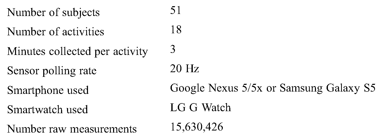
The “WISDM (Wireless Sensor Data Mining) Smartphone and Smartwatch Activity and Biometrics Dataset” [19] include data collected from 51 subjects, each of whom were asked to do 18 tasks for 3 minutes each. Each subject had a smartwatch placed on his/her dominant hand and a smartphone in their pocket.
The data collection was controlled by a custom-made app that ran on smartphones. The sensor information was gathered, from the accelerometer or gyroscope on both the smartphones and smartwatches, yielding four total sensors. The sensor data was collected at a rate of 20 Hz (i.e., every 50 ms). The smartphone was either the Google Nexus 5/5X and Samsung Galaxy S5. The smartwatch was the LG G Watch running Android. The general characteristics of the data and data collection process are summarized in Tab. 1.
Table 1: Summarized information for the data set
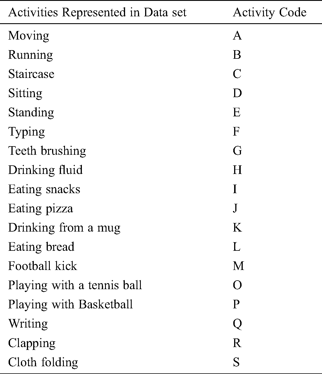
Tab. 2 lists the 18 activities that were performed. The actual data files specify the activities using the code from Tab. 3. Similar activities are not necessarily grouped (e.g., eating activities are not all together). This mapping can also be found at the top level of the data directory in activity_key.txt.
Table 2: The 18 activities represented in data set
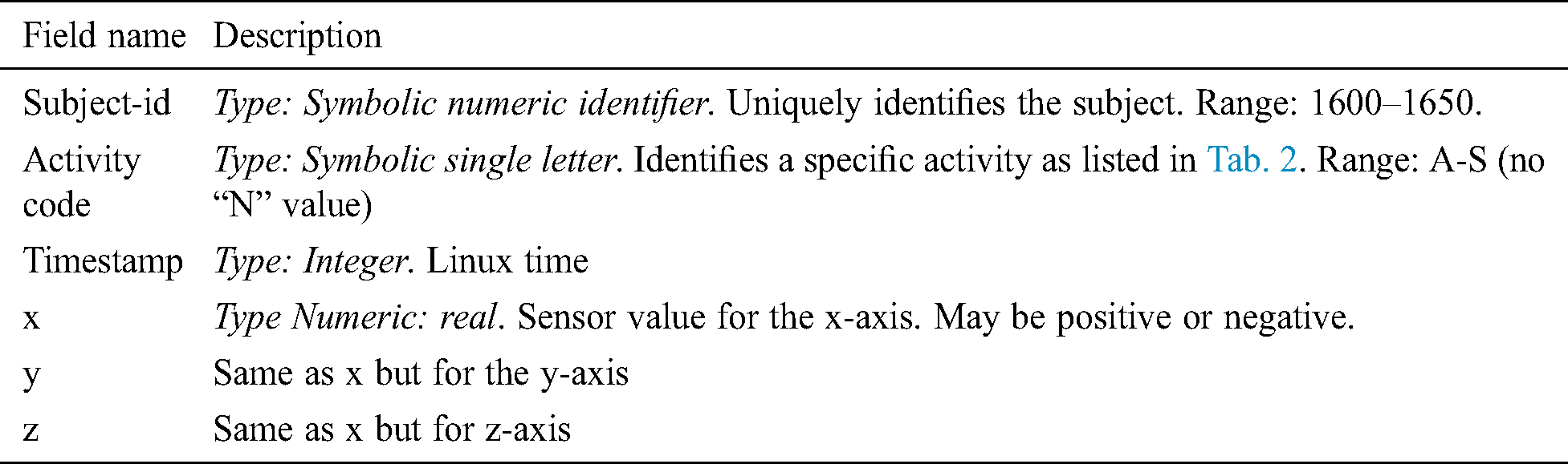
The filename “data_1600_accel_phone” corresponds to the time-series sensor data for subject 1600 from his/her phone accelerometer. The file contains 64,311 lines/sensor readings. Given a sampling rate of 20 Hz, this corresponds to 53.59 minutes of data, which is very close to the expected 54 (18 × 3) minutes of data. If precisely 54 minutes of readings were recorded, that would correspond to 64,800 lines). If we look at the first three lines in the “data_1600_accel_phone” file, we see the following, which corresponds to walking (code A in field 2) activity data.
Table 3: Elements in raw data measurements
3.2.1 The Data Transformation Process
The primary data transformation process utilized to form the labeled examples provided with this data set has been used by our WISDM Lab. It has been used in many research papers, although generally on smaller data sets.
The raw time-series data for each sensor (per subject and activity) is divided into 10-second non-overlapping segments and then based on the 200 (10 s @ 20 reading/s) readings, high-level features are generated contained within each section. A 10-second window was chosen because it provided a sufficient amount of time to capture several repetitions of those activation’s that involve repetitious movements, and still is small enough to offer a quick response (i.e., a prediction every 10 seconds).
However, the examples included in this data set have 93 features (with the label), because some experimentation was done, and additional features were added but never used in published research.
Our transformed examples are placed into ARFF (Attribute-Relation File Format) files, which is a file format specified by the WEKA suite of data mining tools [20]. ARFF files contain both formatting information for the data and then the data itself. The formatting information specifies the information about all the attributes, so we will use the ARFF header to introduce and describe the features generated by the transformation process.
The remainder of the header, starting with line 3 in data. The header goes from line 3 to line 95, with one attribute per line, and thus we get 93 attributes/features. Every line in the header from line 3 to line 95 will begin with “@attribute”. The first column specifies the corresponding line number in the ARFF file. The second column specifies the name of the attribute, which follows the “@attribute” text that starts each line. The attribute name is always included in double-quotes. The third column specifies the attribute type, or, in the case of a categorical feature, a list of all possible feature values. This information follows the attribute name on the line. Some of the attributes/features have many variants (e.g., several have a value per axis so come in multiples of three), so in some cases, the table entries are compressed into a single row (but with multiple line numbers in the first column). For example, feature X0 appears on line 4, X1 on line 4, and X9 on line 13. Similarly, XAVG is on line 34, YAVG on line 35, and ZAVG on line 36 and so on.
@attribute “class”{1601}
@inputs “ACTIVITY”, “X0”, “X1”, “X2”, “X3”, “X4”, “X5”, “X6”, “X7”, “X8”, “X9”, “Y0”, “Y1”, “Y2”, “Y3”, “Y4”, “Y5”, “Y6”, “Y7”, “Y8”, “Y9”, “Z0”, “Z1”, “Z2”, “Z3”, “Z4”, “Z5”, “Z6”, “Z7”, “Z8”, “Z9”, “XAVG”, “YAVG”, “ZAVG”, “XPEAK”, “YPEAK”, “ZPEAK”, “XABSOLDEV”, “YABSOLDEV”, “ZABSOLDEV”, “XSTANDDEV”, “YSTANDDEV”, “ZSTANDDEV”, “XVAR”, “YVAR”, “ZVAR”, “XMFCC0”, “XMFCC1”, “XMFCC2”, “XMFCC3”, “XMFCC4”, “XMFCC5”, “XMFCC6”, “XMFCC7”, “XMFCC8”, “XMFCC9”, “XMFCC10”, “XMFCC11”, “XMFCC12”, “YMFCC0”, “YMFCC1”, “YMFCC2”, “YMFCC3”, “YMFCC4”, “YMFCC5”, “YMFCC6”, “YMFCC7”, “YMFCC8”, “YMFCC9”, “YMFCC10”, “YMFCC11”, “YMFCC12”, “ZMFCC0”, “ZMFCC1”, “ZMFCC2”, “ZMFCC3”, “ZMFCC4”, “ZMFCC5”, “ZMFCC6”, “ZMFCC7”, “ZMFCC8”, “ZMFCC9”, “ZMFCC10”, “ZMFCC11”, “ZMFCC12”, “XYCOS”, “XZCOS”, “YZCOS”, “XYCOR”, “XZCOR”, “YZCOR”, “RESULTANT”
@outputs “class”
Recall that each of the features is based on the sensor readings of one sensor over a 10-second window.
3.3 Detailed Information about the Data
The transformed examples are stored in a manner analogous to the raw time-series data files, with the only difference being that the file names end with “.arff” rather than “.txt”. That is, the data files are stored in a directory structure identical to that shown earlier in Fig. 1, except that the data is stored under a directory called “arff_files” rather than “raw”. Thus, the transformed examples for the phone accelerometer sensor are found under “arff_files/phone/accel,” and that subdirectory will have 51 files corresponding to the 51 subjects. The phone accelerometer examples for subject 1600 will be found in the following file in this subdirectory: data_1600_accel_phone.arff. The arff extension indicates that the file is a valid “arff” file, as specified by the Weka Data Mining Toolkit [20].
The actual number of examples in each subdirectory is provided below:
arff_files/phone/accel: 23,173
arff_files /phone/gyro: 17,380
arff_files /watch/accel: 18,310
arff_files /watch/gyro: 16,632
We expect to have 45.9 hours of examples per sensor (since there are 51 subjects performing 18 activities for 3 minutes per activity). To determine the number of 10-second intervals in 45.9, we multiply 45.9 by 60 (minutes/hour) and then by 6, since there are six 10-second intervals in a minute. This yields 16,524 examples. We see that it is about what we have for three of the four sensors, although we have more for the phone accelerometer, which is consistent with what we say with the raw time-series data.
The primary structure of this algorithm is a generational GA, where every generation has applied the means of determination, hybrid, transformation, and substitution [21]. Every chromosome speaks to a lot of span classification rules. Every classification rule is made out of a lot of traits and class esteem. Each trait in the standard has two genuine factors which show the base and most extreme in the scope of legitimate qualities for that characteristic.
A ‘don’t care’ condition happens when the most extreme value is not exactly the base value. We utilize a fixed-length chromosome, where every chromosome is comprised of a fixed number (n) of rules. The length of a chromosome is in this way n(2A + 1). We instate all the chromosomes at irregular, with values between the scope of every factor. The choice instrument is to pick two people indiscriminately between all the chromones of the populace [22].
In the crossover part, we apply a necessary arbitrary 2-point hybrid crossover. Two mutation operators are utilized in this research. First downer mutation is used to each property's base and most extreme incentive with a probability indicated as the creep rate; at that point, necessary variation replaces arbitrarily chosen trait to go qualities or class values with irregular varieties structure the legitimate fitting range.
In the assessment part, when each quality incentive in an information case is either contained in the range determined for the relating property of a standard or the standard characteristic is a do not care, the rule matches the occurrence, and the class value shows the participation class of the occasion.
The fitness of a chromosome is just the level of test occasions adequately characterized by the chromosome's ruleset (exactness). We generally keep up the best chromosome of the populace as in the elitist conspire.
Parameters Used:
– Number_of_Generations: Is the number of Generations? It is an integer value that indicates the maximum number of generations (or iterations) for the algorithm.
– Population_Size: Is the population size. It is an integer value that determines the number of chromosomes in each generation.
– Cross_Probability: Is the probability of applying the modified simple crossover. It is a float value between 0 and 1.
– Mutation_Probability: Is the probability of utilizing the creep mutation. It is a float value between 0 and 1, and it should have a high value because creep mutation is intended to occur often.
4.1 Generated Rule Set Using Genetic Algorithm for the Subject 1600
There are 20 rulesets generated by the classifier [23] using a genetic algorithm [24] for each subject. As there are a total of 51 subjects, then a total of 1020 rules generated. Due to the space complexity, we are presenting here only two rules generated for the subject 1600.
1: “X2” = [0.12066985017635623, 0.8454452450027329] AND “X3” = [0.33026965528965685, 0.8113940036416506] AND “X7” = [0.00135234832911574, 0.0026779765537190197] AND “X8” = [0.0, 0.0] AND “X9” = [0.0, 0.0] AND “Y0” = [0.015118058439138824, 0.10622135879151089] AND “Y4” = [0.3238220716183591, 0.450288473966133] AND “Y8” = [0.05663211850371028, 0.0988214473400315] AND “Y9” = [0.07713549754049989, 0.10450832914666] AND “Z0” = [0.4011980400342024, 0.4176386092015632] AND “Z6” = [0.005168854811966618, 0.005887896955452835] AND “Z7” = [0.00315953332305875, 0.008851301353157336] AND “Z8” = [0.002556780015015225, 0.004483347160155733] AND “YAVG” = [8.715059835747663, 9.679056631394335] AND “XPEAK” = [44.52408273564291, 47.66813462367769] AND “YSTANDDEV” = [0.19100625519121042, 0.4532833830998382] AND “XMFCC0” = [–0.03549532408195882, 0.37646318643793564] AND “XMFCC1” = [0.3644290711294323, 0.5647424844480977] AND “XMFCC2” = [0.27048488070333615, 0.31981150362217464] AND “XMFCC3” = [–0.13396471949244795, 0.3130277870760335] AND “XMFCC4” = [0.14977918374767274, 0.5746765082333831] AND “XMFCC6” = [0.37224713268348153, 0.6455714149657314] AND “XMFCC7” = [–0.03713547269947956, 0.4275076231240331] AND “XMFCC8” = [0.5106071644903356, 0.5401269541389933] AND “XMFCC11” = [–0.04544265459300431, –0.042691049072687975] AND “XMFCC12” = [0.5346783454010056, 0.6077773546366083] AND “YMFCC3” = [0.6353977425358902, 0.6908368983227242] AND “YMFCC4” = [0.43255994397658015, 0.6795287063255416] AND “YMFCC5” = [0.5133082769044541, 0.519510675604742] AND “YMFCC7” = [0.553251252015277, 0.6692015659892068] AND “YMFCC8” = [0.436812058974823, 0.6021338564090382] AND “YMFCC9” = [0.5142408562386085, 0.5730395899423211] AND “YMFCC10” = [0.31284424004924655, 0.5291414125706504] AND “YMFCC12” = [0.3272221301632445, 0.39210577895471754] AND “ZMFCC0” = [0.0073373376657890205, 0.1142745773693259] AND “ZMFCC2” = [0.12763401518522127, 0.3782890973946903] AND “ZMFCC6” = [0.4750652147766606, 0.5616763966762961] AND “ZMFCC7” = [0.03867950506424854, 0.16380804433658896] AND “ZMFCC8” = [0.13985282647518624, 0.4785053645165013] AND “ZMFCC9” = [0.20466019689186826, 0.48071106654101714] AND “ZMFCC12” = [0.10311453418659068, 0.3018839374007145] AND “XYCOR” = [–0.4918748480418891, 0.3905264839845026] AND “XZCOR” = [–0.6521370853118476, –0.4619792074501847] AND “YZCOR” = [–0.24208802145127428,–0.11771472321823262]: =>1600
2: “X1” = [0.5636900916145393, 0.9524757920188075] AND “X5” = [0.004430757941312799, 0.008021779276435678] AND “X8” = [0.0, 0.0] AND “X9” = [0.0, 0.0] AND “Y0” = [0.03371596118288952, 0.047938080674022915] AND “Y5” = [0.03949956526968152, 0.4029224930337915] AND “Y6” = [0.05568086276195964, 0.2139835708248391] AND “Y7” = [0.100693056401958, 0.14679888755590628] AND “Y9” = [0.008569419544322747, 0.10176406613592152] AND “Z1” = [0.28616983950048913, 0.5505828250689858] AND “Z4” = [0.38617256944677153, 0.8425941930251648] AND “XAVG” = [–4.924163897164588, 3.4500166430428196] AND “YAVG” = [3.7395444396482067, 8.687031124897189] AND “ZAVG” = [1.4871780698732238, 4.279764360134035] AND “XPEAK” = [41.30367633684055, 42.37749492928123] AND “YSTANDDEV” = [0.1989200677962642, 0.5158862895720446] AND “ZSTANDDEV” = [0.02168716655101568, 0.21368384701667914] AND “YVAR” = [0.09552982938020846, 0.4340969233293973] AND “XMFCC0” = [–0.1847838821801764, –0.13575847624665674] AND “XMFCC1” = [0.11566664928600351, 0.5228971971684315] AND “XMFCC2” = [–0.11239377843945372, –0.09030295311327996] AND “XMFCC3” = [0.1485026564547442, 0.6612677514872837] AND “XMFCC5” = [0.38592662508351516, 0.46949631253849633] AND “XMFCC7” = [0.0680157666072132, 0.5833729150972955] AND “XMFCC9” = [0.16005315805967135, 0.20505752367616342] AND “XMFCC11” = [–0.05600544007805072, 0.5712949316423294] AND “XMFCC12” = [0.05664174421097751, 0.13904349806612604] AND “YMFCC0” = [0.23624892380168055, 0.2773991732963452] AND “YMFCC2” = [0.5311459624707051, 0.6952325412348608] AND “YMFCC3” = [0.33590921081389724, 0.7301367801480012] AND “YMFCC6” = [0.7185905311836285, 0.7234455838213105] AND “YMFCC7” = [0.6244384926545752, 0.6852977464250589] AND “YMFCC8” = [0.3902544493639426, 0.6149877534698043] AND “YMFCC9” = [0.5216092149194432, 0.6185758074851673] AND “ZMFCC0” = [0.1754954953853778, 0.29648981111887324] AND “ZMFCC1” = [0.4894710237641607, 0.6601650897277616] AND “ZMFCC2” = [0.10299405239357998, 0.39897580355220963] AND “ZMFCC7” = [0.18377045317078322, 0.4357385978897527] AND “ZMFCC8” = [–0.03485185923892507, 0.42510799732582966] AND “ZMFCC9” = [0.1662672290747576, 0.2070335666645985] AND “ZMFCC10” = [0.15627581270181615, 0.5995528638725092] AND “ZMFCC11” = [0.07079330829125674, 0.5292348723707814] AND “ZMFCC12” = [0.0608363157243421, 0.1975486768637058] AND “YZCOS” = [–0.8121362605413858, 0.3712944534102286] AND “RESULTANT” = [10.195865707615546, 10.726049484914302]: =>1600
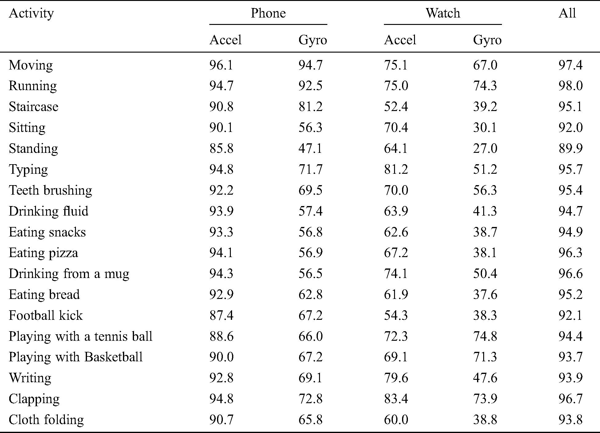
5 Identification Accuracy using One 10-second Slot (RF)
The verification results for the Random Forest algorithm, where rules depend on a solitary 10-second (i.e., without casting), are given in Tab. 4. Results are accommodated every eighteen exercises and every different sensors blends [25]. The overall estimation of the different sensor arrangements can be controlled by looking at the qualities in the various segments.
Table 4: Authentication EER using one 10 s slot (RF)
6 Different Activity Distribution Concerning with Different Attributes in the Dataset
Analysis of the activity distribution with different attributes represented in this section in Figs. 1–12 to get efficient results.

Figure 1: Class distribution with respect to X0

Figure 2: Activity distribution with respect to resultant

Figure 3: X2 distribution with respect to resultant
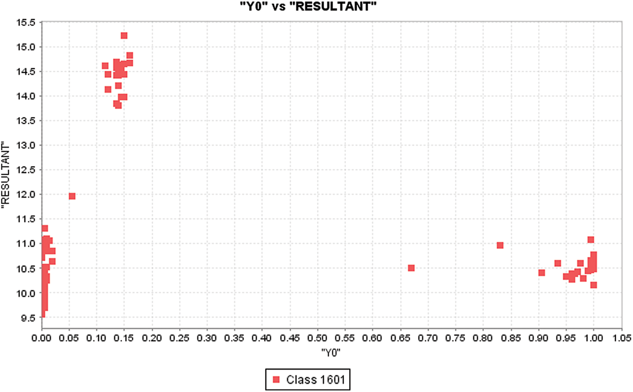
Figure 4: Y0 distribution with respect to resultant
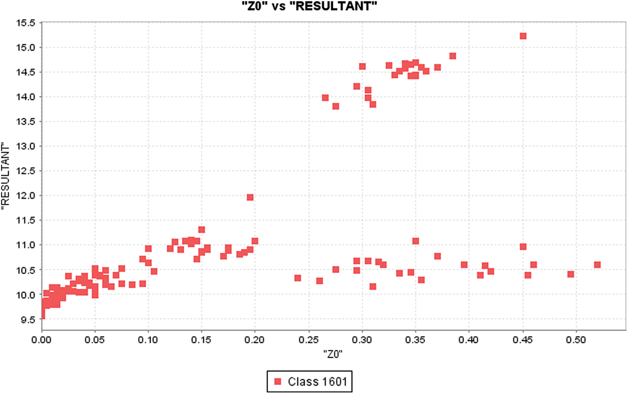
Figure 5: Z0 distribution with respect to resultant
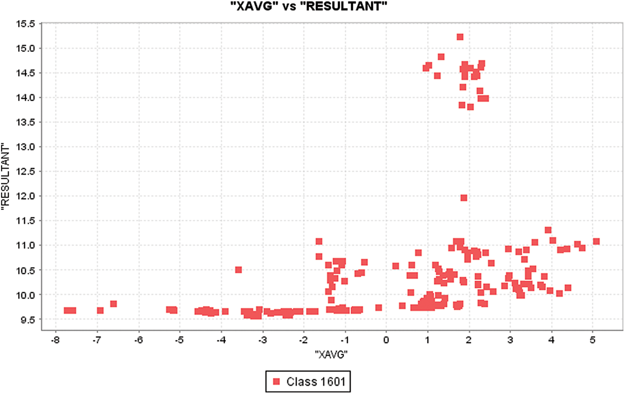
Figure 6: XAVG distribution with respect to resultant
Figure 7: ZAVG distribution with respect to class
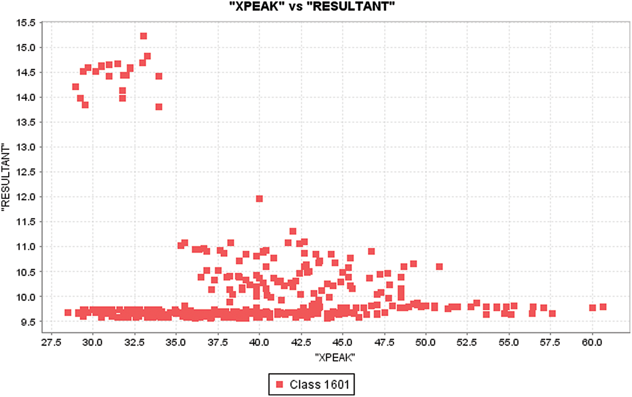
Figure 8: XPEAK distribution with respect to resultant
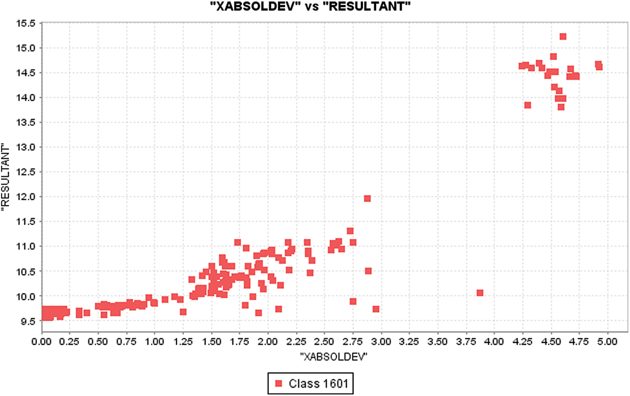
Figure 9: XABSOLDEV distribution with respect to resultant
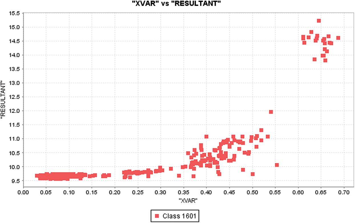
Figure 10: XVAR distribution with respect to resultant
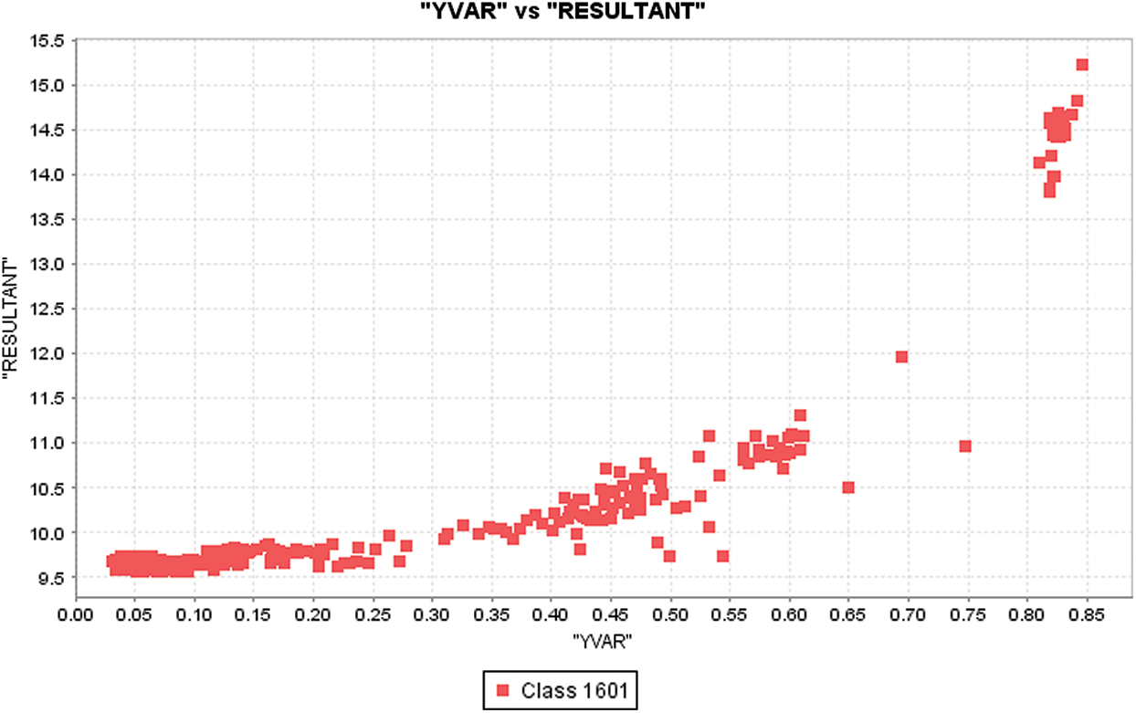
Figure 11: YVAR distribution with respect to resultant

Figure 12: ZVAR distribution with respect to resultant
The feasibility of motion-based biometrics which uses daily routine activities used in smartwatches and phones is analyzed in this research. When the accelerometer/gyroscope sensors on both devices, i.e., smartphones and smartwatch are used together, it gives the better performance of biometric. Usage of 50 seconds of data evolved rather than 10 seconds of data grown improves the biometric working is shown in this paper. There is a sensitivity in biometric performance to the amount of data training. When the maximum amount of trained data is added, the authentication and identification tasks improve fast. The max. of 170 seconds of data/activity was reached, then the improvement continues.
Similarly, the identification performance is also improved, with the 2 minutes of training data/activity began to reach a plateau. The training data increase so overall performance. Most of the studies show the authentication, but this study demonstrates the feasibility of identification in using daily routine activities with fifty-one subjects. As per the model created in the experiment, we can conclude that the maximum accuracy achieved is 98.0% for overall using accelerometer and gyro sensors of a smartphone/smartwatch.
Activities like running, writing, and catching are considered better activities for health. All the 18 activities were evaluated are went quite useful in biometrics and became feasible in daily routine activities. There is feasibility in implementing the two-stage approach where the recognition identified activities. Then the model of biometric authentication is applied to identify/authenticate the subjects.
The research that is demonstrated in this paper can also be used to extend in many essential ways. Employ activity recognition in the 1st stage in the two-staged biometric system that was implemented, and one key can be used to include for other activities.
The interesting fact is to apply and evolve the usage of one class for biometric authentication and identification, which is used by smartphones and smartwatches.
Funding Statement: The authors would like to thank Deanship of Scientific Research at Majmaah University for supporting this work under Project Number No. RGP-2019-26.
Conflicts of Interest: The authors declare that they have no conflicts of interest to report regarding the present study.
1. M. Shoaib, S. Bosch, O. D. Incel, H. Scholten and P. J. Havinga. (2014). “Fusion of smartphone motion sensors for physical activity recognition,” Sensors, vol. 14, no. 6, pp. 146–156. [Google Scholar]
2. A. Khafajiy, M. Baker and T. Chalmers. (2019). “Remote health monitoring of elderly through wearable sensors,” Multimedia Tools Application, vol. 78, no. 17, pp. 24681–24706.
3. G. M. Weiss, K. Yoneda and T. Hayajneh. (2019). “Smartphone and smartwatch-based biometrics using activities of daily living,” IEEE Access, vol. 7, pp. 133190–133202.
4. J. R. Kwapisz, G. M. Weiss and S. A. Moore. (2011). “Activity recognition using cell phone accelerometers,” ACM SIGKDD Explorations Newsletter, vol. 12, no. 2, pp. pp 74–82.
5. E. Frank, M. A. Hall and I. H.Witten. (2016). The WEKA Workbench. Online Appendix for “Data Mining: Practical Machine Learning Tools and Techniques,” Fourth Edition, Morgan Kaufmann. [Google Scholar]
6. G. M. Weiss, J. W. Lockhart, T. T. Pulickal, P. T. McHugh, I. H. Ronan et al. (2016). , “Actitracker: A smartphone-based activity recognition system for improving health and well-being,” in Proc. of IEEE Int. Conf. on Data Science and Advanced Analytics, Montreal, QC, Canada, pp. 682–688. [Google Scholar]
7. X. Su, H. Tong and P. Ji. (2014). “Activity recognition with smartphone sensors,” Tsinghua Science and Technology, vol. 19, no. 3, pp. 235–249. [Google Scholar]
8. X. Su, X. C. Liu, J. C. Lin, S. M. He, Z. J. Fu et al. (2017). , “De-cloaking malicious activities in smartphones using http flow mining,” KSII Transactions on Internet and Information Systems, vol. 11, no. 6, pp. 3230–3253. [Google Scholar]
9. Z. F. Liao, J. X. Wang, S. G. Zhang, J. N. Cao and G. Min. (2014). “Minimizing movement for target coverage and network connectivity in mobile sensor networks,” IEEE Transactions on Parallel and Distributed Systems, vol. 26, no. 7, pp. 1971–1983. [Google Scholar]
10. F. Yu, L. Liu, L. Xiao, K. L. Li and S. Cai. (2019). “A robust and fixed-time zeroing neural dynamics for computing time-variant nonlinear equation using a novel nonlinear activation function,” Neurocomputing, vol. 350, pp. 108–116. [Google Scholar]
11. P. Sharma, K. Saxena and R. Sharma. (2015). “Diabetes mellitus prediction system evaluation using c4.5 rules and partial tree,” in Proc. of 4th Int. Conf. on Reliability, Infocom Technologies and Optimization, IEEE, India, pp. 1–6. [Google Scholar]
12. P. Sharma and K. Saxena. (2017). “Application of fuzzy logic and genetic algorithm in heart disease risk level prediction,” International Journal of System Assurance Engineering and Management, vol. 8, no. Supplement 2, pp. 1109–1125.
13. J. Wang, Y. Gao, W. Liu, A. K. Sangaiah and H. J. Kim. (2019). “An intelligent data gathering schema with data fusion supported for mobile sink in wireless sensor networks,” International Journal of Distributed Sensor Networks, vol. 15, no. 3, pp. 1550147719839581.
14. G. M. Weiss, J. L. Timko, C. M. Gallagher, K. Yoneda and A. J. Schreiber. (2016). “Smartwatch-based activity recognition: A machine learning approach,” in Proc. of the IEEE Int. Conf. on Biomedical and Health Informatics, Las Vegas, NV, pp. 426–429. [Google Scholar]
15. V. Ahanathapillai, J. D. Amor, Z. Goodwin and C. J. James. (2015). “Preliminary study on activity monitoring using an android smart-watch,” Healthcare Technology Letters, vol. 2, no. 1, pp. 34–39. [Google Scholar]
16. Y. Zheng, W. K. Wong, X. Guan and S. Trost. (2013). “Physical activity recognition from accelerometer data using a multi-scale ensemble method,” in Conf. on Innovative Applications of Artificial Intelligence.
17. W. Wang, Y. T. Li, T. Zou, X. Wang, J. Y. You et al. (2020). , “A novel image classification approach via dense-mobilenet models,” Mobile Information Systems, Vol. 2020, pp. 1–8.
18. A. Mannini, S. S. Intille, M. Rosenberger, A. M. Sabatini and W. Haskell. (2013). “Activity recognition using a single accelerometer placed at the wrist or ankle,” Medicine and Science in Sports and Exercise, vol. 45, no. 1, pp. 2193–2207. [Google Scholar]
19. G. Weiss, Computer and Information Sciences Department, Fordham University, 2019. [Google Scholar]
20. J. Wang, X. J. Gu, W. Liu, A. K. Sangaiah and H. J. Kim. (2019). “An empower hamilton loop based data collection algorithm with mobile agent for WSNs,” Human-centric Computing and Information Sciences, vol. 9, no. 1, pp. 1–14. [Google Scholar]
21. R. Samikannu, R. Ravi, S. Murugan and B. Diarra. (2020). “An efficient image analysis framework for the classification of glioma brain images using CNN approach,” Computers, Materials & Continua, vol. 63, no. 3, pp. 1133–1142. [Google Scholar]
22. J. Alcala, A. Fernandez, J. Luengo, J. Derrac, S. García et al. (2011). , “Keel data-mining software tool: Data set repository, integration of algorithms and experimental analysis framework,” Journal of Multiple-Valued Logic and Soft Computing, vol. 17, no. 2, pp. 255–287. [Google Scholar]
23. I. Triguero, S. González, J. M. Moyano, S. García, J. Alcalá-Fdez et al. (2017). , “Keel 3.0: An open source software for multi-stage analysis in data mining,” International Journal of Computational Intelligence Systems, vol. 10, no. 1, pp. 1238–1249. [Google Scholar]
24. J. Wang, Y. Q. Yang, T. Wang, R. S. Sherratt and J. Y. Zhang. (2020). “Big data service architecture: A survey,” Journal of Internet Technology, vol. 21, no. 2, pp. 393–405. [Google Scholar]
25. U. John, K. Kumar, K. Wook and L. Lu. (2020). “Wearable sensor monitoring and data analysis,” United States Patents. [Google Scholar]
 | This work is licensed under a Creative Commons Attribution 4.0 International License, which permits unrestricted use, distribution, and reproduction in any medium, provided the original work is properly cited. |