DOI:10.32604/cmc.2021.012466
| Computers, Materials & Continua DOI:10.32604/cmc.2021.012466 | |
| Article |
Recognition and Classification of Pomegranate Leaves Diseases by Image Processing and Machine Learning Techniques
1School of Computer Science Engineering, Lovely Professional University, Punjab, 144411, India
2University of Economics Ho Chi Minh City, Ho Chi Minh City, 70000, Vietnam
3Maharaja Agrasen Institute of Technology, 110086, India
*Corresponding Author: Aditya Khamparia. Email: aditya.khamparia88@gmail.com
Received: 01 July 2020; Accepted: 07 August 2020
Abstract: Disease recognition in plants is one of the essential problems in agricultural image processing. This article focuses on designing a framework that can recognize and classify diseases on pomegranate plants exactly. The framework utilizes image processing techniques such as image acquisition, image resizing, image enhancement, image segmentation, ROI extraction (region of interest), and feature extraction. An image dataset related to pomegranate leaf disease is utilized to implement the framework, divided into a training set and a test set. In the implementation process, techniques such as image enhancement and image segmentation are primarily used for identifying ROI and features. An image classification will then be implemented by combining a supervised learning model with a support vector machine. The proposed framework is developed based on MATLAB with a graphical user interface. According to the experimental results, the proposed framework can achieve 98.39% accuracy for classifying diseased and healthy leaves. Moreover, the framework can achieve an accuracy of 98.07% for classifying diseases on pomegranate leaves.
Keywords: Image enhancement; image segmentation; image processing for agriculture; K-means; multi-class support vector machine
In agricultural production, cultivation plays an essential role in ensuring food security for each country. Most of the people involved in crop activities of the rural areas usually have limited knowledge of plant diseases, which is a major cause of crop failure. The plant disease becomes visible to farmers at a very late stage. Therefore, farmers with limited knowledge of plant diseases usually choose chemical pesticides and fertilizers, which affect the soil’s minerals and cause pollution.
The identification of disease in plants plays a significant role in the field of agriculture. Automatic plant disease identification is useful to classify plant diseases and define a kind of disease. Many plant diseases were discovered. They are very dangerous for plants and can kill them in a short time. For example, a disease on leaves of pine trees was founded in the U.S. The disease affects plants by inhibiting their growth and causing them to die within six years. It became prevalent in the southern regions of the United States, especially in the state of Alabama. Early diagnosis may have been beneficial in the scenario. Using experts to identify plant diseases is a popular method. However, the method is expensive. Moreover, many countries lack expert teams, either the farmers lacking in scientific knowledge are very hard to absorb suggestions from the experts. Even when farmers receive expert advice, they worry about costs and time, and above all, it requires a long time to monitor the plants. Therefore, we proposed a framework to solve these drawbacks. The framework focuses on monitoring a large area of crop automatically. Automatic disease detection will provide a more straightforward and cheaper solution than using many experts. It also can monitor, store, and analyze the data automatically [1–4]. Plant illness recognition by naked eyes is not simple. Also, the accuracy of the method depends much on the knowledge of experts.
There are several common plant diseases such as brown or yellow spots, fungal, viral, and bacterial diseases at an early and late stage. Experts will identify a plant illness by looking at the infected regions, the change of leaf color, or other parts of the plants such as trunk trees and branches of trees. To develop an automation method for detecting plant diseases, we use the same way: Assess important features of leaves of plants by using image processing and analysis techniques [5].
For the preprocessing step, we use image enhancement to improve color contrast. Another image processing used in this work is image segmentation. Image segmentation plays a crucial role in distinguishing regions affected by a disease and other healthy parts of the leaf. There are many image segmentation methods that we can use here, such as thresholding methods, level-set method methods, watershed methods, and cluster-based methods [6]. After implementing the segmentation task, a specific portion of the image will be extracted for identifying a plant disease. Based on segmented regions, one can extract essential features such as color detail and boundaries for diagnosing diseases [7,8].
In the designed framework, we used a K-Means algorithm for color image segmentation. After completing the image segmentation task, image classification is applied. Support Vector Machine (SVM) can be used for image classification, but it is only efficient for the problem dealing with a binary decision, i.e., data can be divided into two independent classes. However, the data dealing with this problem relates to five categories, so the image classification method must be done with multiple classes. Hence, the solution to this problem needs to be a multi-class SVM.
The study focuses on a specific fruit tree instead of working on many kinds of plants to identify plant diseases more accurately. Because various diseases can affect many plants, the study can be extended to apply for other kinds of trees easily. Maintaining accuracy for a specific crop will bring more significant benefits to the farmers. In this article, we motivate study on pomegranate because it is one of the most popular fruit trees in India, and its output is about 740 billion tons per year.
2 An Overview of Plant Diseases Identification
Sladojevic et al. [9] recognized the plant diseases and classifying them using convolutional neural networks (CNN). The study’s precision is between 91 percent and 98 percent for a specific disease, and the average precision was 96.3 percent. Singh et al. [10] proposed another method for plant disease identification using leaf images of plants by using a genetic algorithm. The method utilized some image processing techniques such as image acquisition, image segmentation, and feature extraction. Some other approaches were used for this problem, such as artificial neural networks (ANN), Bayes Classifier, Fuzzy Logic, and some hybrid algorithms. Khirade et al. [11] proposed a method for the recognition of plant illness using ANN. Kirani et al. [12] developed another method to recognize infectious plants based on fuzzy logic. Fuzzy logic is used for classifying and optimizing the model. This method is well-known as an application for botany. The accuracy of the method is around 93 to 96 percent. Singh et al. [13] combined a genetic algorithm with K-Means clustering and SVM to propose a method for detecting and classifying plant diseases. The purpose of the genetic algorithm is to optimize the fuzzy parameters of the model. Accuracy the method with Minimum Distance Criterion is about 93.6 percent, and SVM is about 95.7 percent. Golhani et al. [14] used various types of neural networks to recognize plant disease using hyperspectral data. The neural network techniques are essential to process thermographic data. There are various types of single-layer neural networks, multi-layer neural networks, radial basis function, Kohonen’s self-organizing map (SOM), probabilistic neural network (PNN), and convolutional neural networks (CNN), and feed-forward and back-propagation neural networks. Mattihalli et al. [15] proposed a framework in terms of IoT (Internet of Things) to recognize plant diseases and integrated with many other functions that allow the system can spread drugs to treat the diseases automatically if the plant is in the primary stage of infection. The information can be monitored through GSM (Global System for Mobile Communications). Pantazi et al. [16] proposed an automated method of recognizing plant illness using Local Binary Patterns (LBPs) for feature extraction and One-Class Classification and then classified the plant diseases including black rot, downy or powdery mildew and healthy. The accuracy achieved about 95 percent, with a total sample of 46. Some advanced techniques for recognizing plant diseases are molecular techniques, spectroscopic imaging techniques, and profiling of plant volatile organic compounds [17]. Molecular techniques include PCR, ELISA, and Hybridization [18]. Spectroscopic imaging techniques include Fluorescence spectroscopy, Visible and Infrared spectroscopy, Fluorescence imaging, hyperspectral imaging. The systems that deal with profiling of plant VOC are electronic nose systems and GC-MS.
The significant research gap found in the above works is to generalize all crops as a single scenario in which the diseases might affect plants with various levels. So, in this scenario, the efficiency of defining disease is more important. Using machine learning techniques, we can only achieve an accuracy of 95.7% in a general case, but we can achieve better accuracy for a specific plant. The reasons, as mentioned earlier, are the main philosophy considered behind all the work.
The dataset utilized for the experimentation is of hybridized data collected from various sources. The dataset used consists of pomegranate leaves’ images. This dataset contains the following types of images:
1. Healthy leaves: These leaves do not have any infection and are green in color.
2. Alternaria Alternata infected leaves images: These are a fungus that causes dark spots on plant parts and rots them.
3. Anthracnose: For this disease, dark and sunken type lesion is visible on leaves. It is an infection caused by fungus.
4. Bacterial Blight: It is a bacteria-infected disease in which pale green spots appear on leaves and in later stage leaf appear water-soaked.
5. Cercospora Leaf Spot: Black dots and grayish tanned lesions appear on the leaf.
The methods are used in the implementation of leaf disease detection for pomegranate using leaf images are K-Means algorithm and multi-class SVM, and image processing techniques like image enhancement and segmentation. The plant disease detection process is implemented in two phases, as follows:
Disease detection: This phase of the process implemented by using image processing techniques. In this phase, the K-Means algorithm utilized for clustering the infected regions on the plant leaves images, as shown in Fig. 1. In the disease detection phase, the two significant steps: image enhancement and image segmentation, were implemented. Image enhancement: Enhancing an image is very important to make the features properly visible and identifiable. For a color image, it has been done by using several methods such as image resizing, enhancing colors of the images, and converting the plant leaf image in RGB color space into the Luminosity, as in Fig. 2. For black and white images, this task can do by using histogram equalization. Image segmentation: It refers to a process of deriving useful features from the image. The mentioned step is the essential step for identifying the infected surface from the plant leaf. This task can solve by using the K-Means algorithm, as shown in Fig. 3.
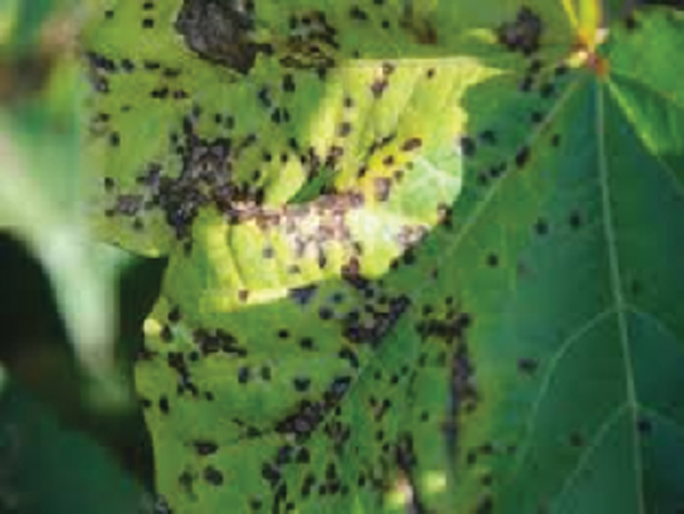
Figure 1: Input image of infected leaf
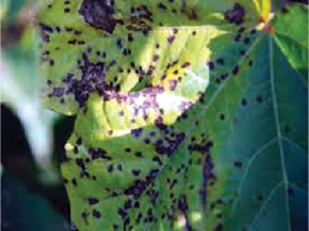
Figure 2: Enhanced image of the leaf to better identify the infected parts
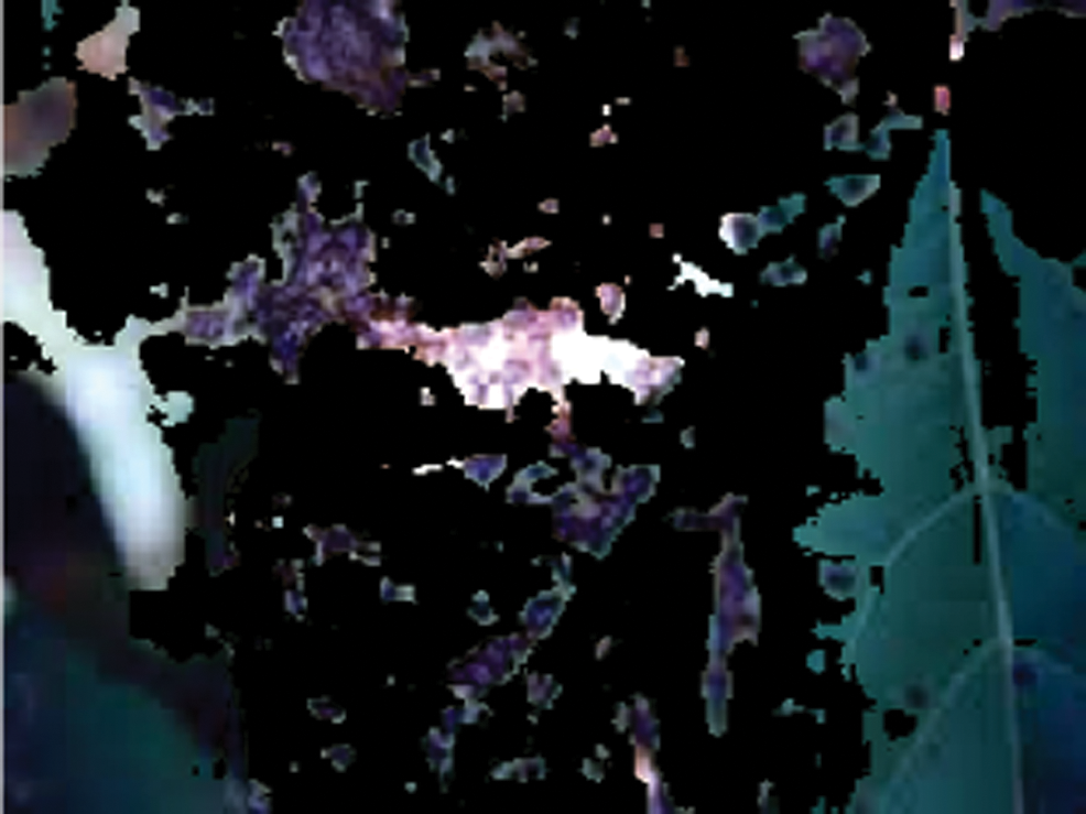
Figure 3: Segmented image showing the infected parts
Disease classification: This phase of the process deals with classifying the detected disease. It means that we must define which class based on the labels belongs to the plant disease–-The mentioned task is implemented using a multi-class SVM algorithm.
4.1 Algorithm Based on K-means Clustering for Disease Recognition
The need to use the K-Means clustering in this implementation is to identify clusters of diseased spots on the leaf and further. There was not any prior knowledge about those clusters or patterns. Therefore, we choose the K-Means algorithm. The following steps are:
Step-1: The number of clusters (K) to be determined (depending on the necessity, we can vary K value and repeat the whole process).
Step-2: The number of centroid values to initiated randomly, representing each centroid value for each cluster. The number of values considered depends on the determined K.
Step-3: The Euclidean distance between different points and centroids of each cluster will evaluate.
Step-4: Depending on the distance, reform the clusters and calculate the new centroid for each cluster.
Step-5: Repeat Steps 3 and 4 until there is not much change in the centroids and return those centroids.
4.2 Mathematical Support of K-means Algorithm
K-Means algorithm used for the clustering of the points depending on the similarity and dissimilarity. Proximity measures measure similarity and dissimilarity. In this scenario, the proximity measure considered to be distance. The popular distances used in machine learning are:
1. Minkowski Distance can be calculated as in Eq. (1):

where  ,
,  and
and  represents the Minkowski distance between X and Y.
2. Manhattan Distance can be calculated as in Eq. (2):

where  ,
,  , and
, and  represents Manhattan distance between X and Y.
3. Euclidean Distance can be calculated as in Eq. (3):

where  ,
,  , and
, and  represents the Euclidean distance between X and Y.
One can understand that the Minkowski distance is more generalized, while the other distances can be easily derivable from Minkowski distance. Besides identifying the proximity measure, there was a need to identify the optimized values for K, representing the number of clusters in which whole data points can divide. There are two methods, such as the Elbow method and the Silhouette Method, to identify the optimized K value. Elbow method purely based on the graphical scenario in which made to draw a graph between the number of clusters and sum of squares within the cluster, from an absolute value of K, the variation will be less such K values considered as an optimized value for K. Silhouette method, again purely based on analytical support. In this method, the Silhouette coefficient will calculate for different K values. For each K value, the average Silhouette coefficient and K value will select for which the maximum Silhouette coefficient occurs, that K value is considered optimal. Mathematical formulae can provide as in Eqs. (4)–(6):


where Ci is the ith data point assigned cluster,  is the number of data points assigned to cluster i, ai is the measure of similarity in which ith data point assigned, bi is the average measure of dissimilarity with the closest cluster to which the point is not assigned, and Si is the Silhouette coefficient. Other feature statistics are also used in this implementation, such as mean, standard deviation, entropy, root mean square, variance, skewness, kurtosis, contrast, correlation, and energy for identifying variations in the images.
4.3 The Algorithm Used for Disease Classification: Multi-Class SVM
According to the framework, the clustering of the points made by utilizing the K-Means algorithm. The classification of plant diseases depends on the patterns that are available on the leaf images. Supervision is needed for such classification to let the machine can understand the pattern and classifying them. There are many algorithms for the classification of supervised learning purposes, but we choose SVM because it can capture complex relations among the datapoints very easily without intensive computations and a more extended period of training. Now, an issue with the SVM is that it only can classify the data into two classifiers inherently, but we need to classify data into more than two categories. So, the plan shifted from SVM to multi-class SVM. SVM can utilize for both linear classification and non-linear classification. The significant advantage of this method is using kernel functions as decision functions. The different kernel functions are available such as linear, polynomial, gamma, sigmoid functions, and customized kernel functions. In the implementation, the linear kernel function used.
4.3.1 Mathematical Support of Multi-Class SVM
SVM is a supervised learning technique. Initially, it was a technique used for the classification of binary-class data. As time is turning around, the technology was improved to make SVM work on multi-class data.
If data is of two categories and graphically or algebraically a line or plane can separate the data into two categories, then such data is known as linear separable. A line or plane which divides the data into two categories is known as a hyperplane. If the data is of one dimensional, then the hyperplane will be a point. If the data is two-dimensional, then the hyperplane will be a line if the data is n-dimensional, where  , then the hyperplane will be a plane. Then, the mathematical representation of SVM for binary categorical data considered. There are two parts in SVM to get the hyperplane, which can divide the data more optimally. They are:
1. Finding all possible set of hyperplanes.
2. Find out the optimal hyperplane of all the hyperplanes.
These two steps included in the mathematical representation. For better understanding, the two-dimensional data space considered so that one can understand that the hyperplane will be a line. A line mathematically can be represented as in the Eq. (7):

where  and
and  .
.
Similarly, a hyperplane can be represented in n-dimensional data space where W will be a column matrix of  , and X will also be a column matrix of size
  and will be represented in the form as WTX + B = 0. For classifiers, the hypothesis will be defined in that the hyperplane will divide the data space into two parts in two-dimensional space. The hypothesis
  will be defined as in Eq. (8):

In this instance, one can observe that there will be a more significant number of hyperplanes that exist without restrictions, it is necessary to identify the optimal hyperplane of all the hyperplanes. The above mentioned two parts of the hypothesis can combine into a single expression as in Eq. (9):

Let us suppose yi =+1 represents a hyperplane in the above equation and denote it by H1 and yi = −1 represents another hyperplane in the above equation and denote it by H2. Now, the distance between H1 and the origin will be  and distance between H2 and the origin is
  . So, the margin can be identified. For optimal hyperplane, the distance between margins needs to be maximized and the origin, which means to maximize
  or minimize
  or
or  . Therefore, we can achieve the optimal hyperplane.
For multi-class SVM, there are two ways to solve it: construct several binary classifiers and combine them and consider the complete data and formulate the optimization problem. These methods are costly for computation due to a large number of variables. For the same reason, there are three different approaches for solving multi-class SVM as One-versus-All, One-versus-One, and DAGSVM (Directed Acyclic Graph Support Vector Machine) methods. In the case of the first method, the model will be constructed such that there will be many SVM models as many as the number of categories or classes exists in a particular feature of the data. Then, many hypotheses will be defined as many as the number of classes in a feature. In each case of the hypothesis will be defined them corresponding to each category or class. If an entity belongs to a class corresponding to that hypothesis, it will be considered positive, and the remaining is unfavorable, and this process will be applied to every other hypothesis. Let us suppose there are m classes that imply the need to consider m SVM models. Consider the kth model for training activity with all the samples in that class with positive tags and the other with negative tags. Let the training data be the size of p  ,
,  , where
  ,
,  and
and  will be the class of xi, and the kth model can be solved as in Eq. (10):

where function  maps, xi, the training data into higher dimensional data space and C is a penalty parameter. The optimization, as mentioned earlier, the problem is in the higher dimensions of the simple SVM model due to more categories; otherwise, both are one another the same. By solving the above equation, m decision functions will attain, and the generalize equation can mention in the first part as that of Eq. (11), then,
  will consider overall the m equations obtained as mentioned in the second part of Eq. (11).

In the second method, a pair of classes will be considered and try to develop a binary classification among all the classes. Suppose that there are n classes and every time, a pair of classes will be considered to create a binary classification, then the number of classifiers will be  . Let us suppose that the ith and jth classes for constructing binary classification problems can be represented in Eq. (12):


The voting process will take the data point allocation to a certain class, i.e., if  says that the data point belongs to the ith class, then the number of votes for the ith class will be incremented by 1 else jth class will be incremented by 1. Finally, which class got the majority votes to that class, the data point will be moved. If there is any situation of a tie of votes, the data point will be moved to the class, which has a smaller index. In the third method, the training phase will be similar to the second method, but it varies in the testing phase. In the testing phase, the binary directed graph, which is of acyclic, will be considered with the number of nodes equal to the number of classifiers, i.e.,
  and the number of leaves is equal to the number of classes, i.e., n. Each node in the graph acts as a basic SVM, i.e., binary classification. At each node, the test sample will be provided and check for the binary decision function and depending on that, and the testing data point will be placed into the corresponding class.
Image acquisition is one of the essential phases of the implementation. Whatever the images obtained through this phase will serve as input for the implementation part. Through the acquisition, there are 201 images used for the implementation, in that 126 images, i.e., nearly 63% of the dataset, are used for the training the model and 75 images, i.e., nearly 37% of the datasets, are used for the testing of the model. Different techniques are also utilized in image processing as part of this implementation, such as resizing the image, enhancing color, converting the colored image into grayscale, image segmentation, and extracting features from the segmented image. Image segmentation is a crucial aspect of this implementation for the cluster formation and identification of disease, in that, the path from the root to a leaf gives the information about the classification of the data point or just a predicted class.
4.5 Algorithm for the Leaf Disease Detection
Steps of the algorithm are presented as follows:
Step-1: Applying image processing techniques on the image dataset.
Step-1.1: Gathering of images required for the implementation (image acquisition).
Step-1.2: Preprocessing the images for further use by resizing, enhancing, and converting into grayscale.
Step-1.3: Segmenting the images for identifying infected regions on the leaves.
Step-1.4: Extracting features the images by applying the K-means algorithm.
Step-1.5: Evaluate the regions affected by the disease.
Step-2: Load all the training data features.
Step-3: Classify the images into different categories based on the labels defined by using Multi-Class SVM.
Step-4: Load all the testing data features.
Step-5: Evaluate the accuracy of the model.
4.6 The Flow Chart for the Proposed Methodology
The flowchart of the implementation of the disease’s detection by using pomegranate leaf images is presented as in Fig. 4.
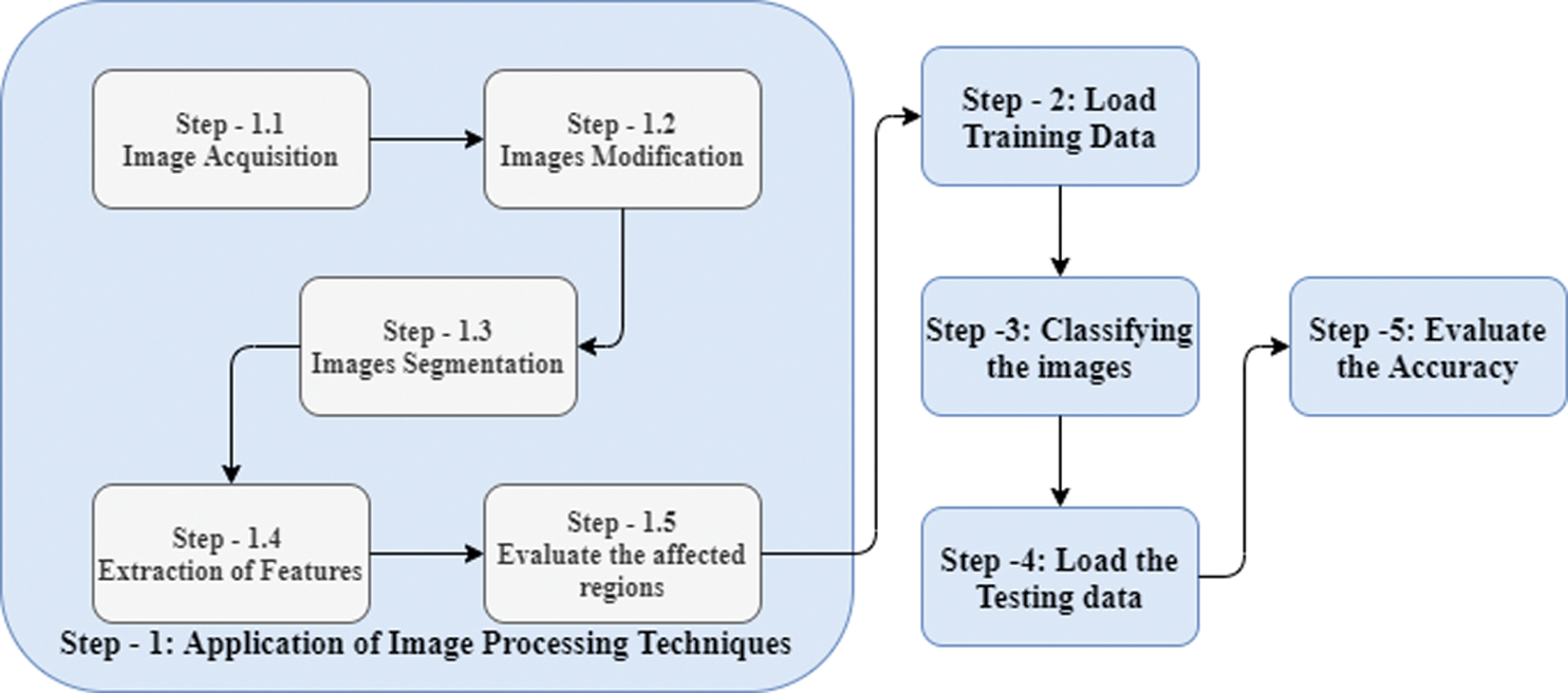
Figure 4: Flowchart for the implemented algorithm
The system configuration includes Operating System–-Windows 10, 64-bit, Processor: Intel® Core™ i3-8130U CPU@2.20–2.21 GHz, Processor capacity: 8.00 GB. Developed environment: MATLAB R2016a. We designed a Graphical User Interface (GUI) to automatically detect diseases using the image of a leaf. The options such as loading image and enhancing the image are the part of image preprocessing, segmenting image is the part of the identification of infected region, classification result will classify the disease based on the patterns of the identified infected region on the leaf image, the tool also calculates the percentage of an area on the leaf infected, the accuracy of the classification result, and features mentioned in Section 4.1.1. In the case of image segmentation, the system will generate three different regions for image segmentation to let people select an appropriate region for identifying the disease, as in Fig. 5.
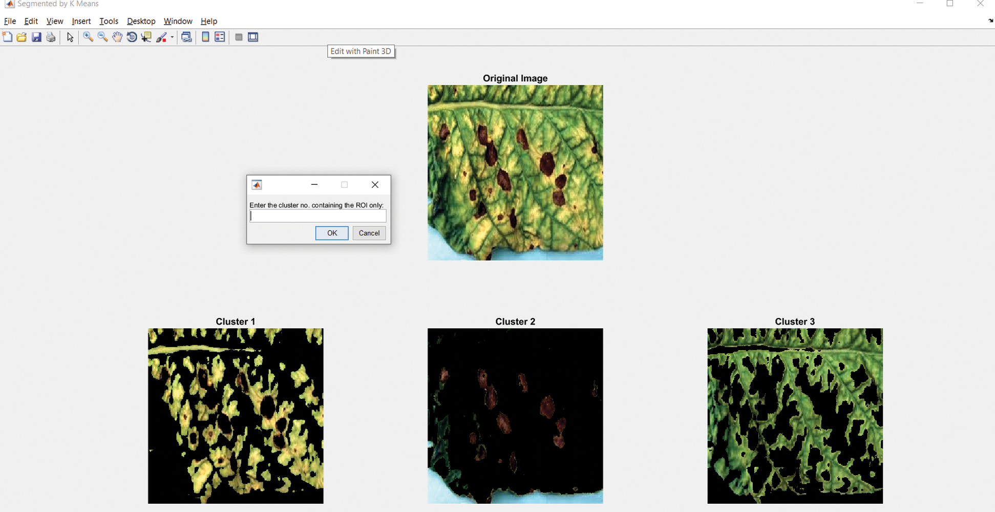
Figure 5: Image segment window with option selecting the infected region
In this section, the results of recognizing the pomegranate plant diseases into five different categories discussed. They are Alternaria Alternata, Anthracnose, Bacterial Blight, Cercospora Leaf Spot, and Healthy Leaves.
6.1 Results in Case of Alternaria Alternata
Fig. 6 shows the GUI of the proposed framework for the implemented scenario. In the case of Alternaria Alternata, the accuracy obtained by the framework of about 98.39%.
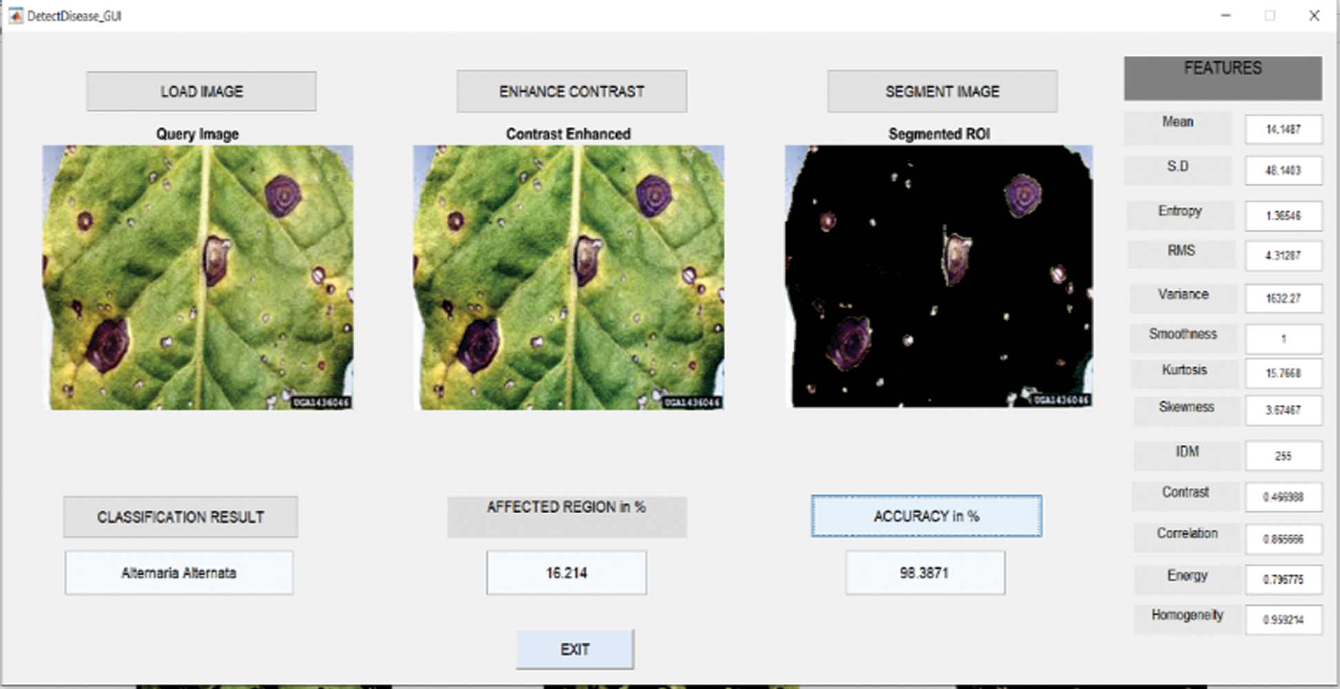
Figure 6: GUI for alternaria alternata
6.2 Results in Case of Anthracnose
Fig. 7 shows the GUI of the proposed framework for the implemented scenario. In the case of Anthracnose, the accuracy obtained by the framework of about 98.39%.
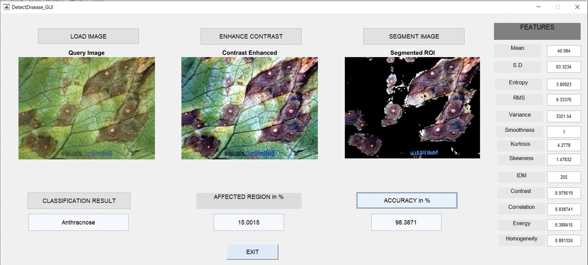
Figure 7: GUI for anthracnose
6.3 Results in Case of Bacterial Blight
Fig. 8 shows the GUI of the proposed framework for the implemented scenario. In the case of Anthracnose, the accuracy obtained by the framework of about 98.39%.
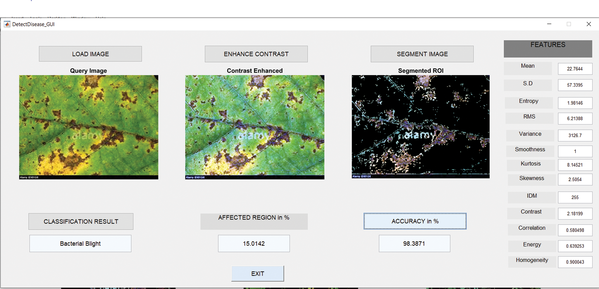
Figure 8: GUI for bacterial blight
6.4 Results in Case of Cercospora Leaf Spot
Fig. 9 shows the GUI of the proposed framework for the implemented scenario. In the case of Anthracnose, the accuracy obtained by the framework of about 96.77%.
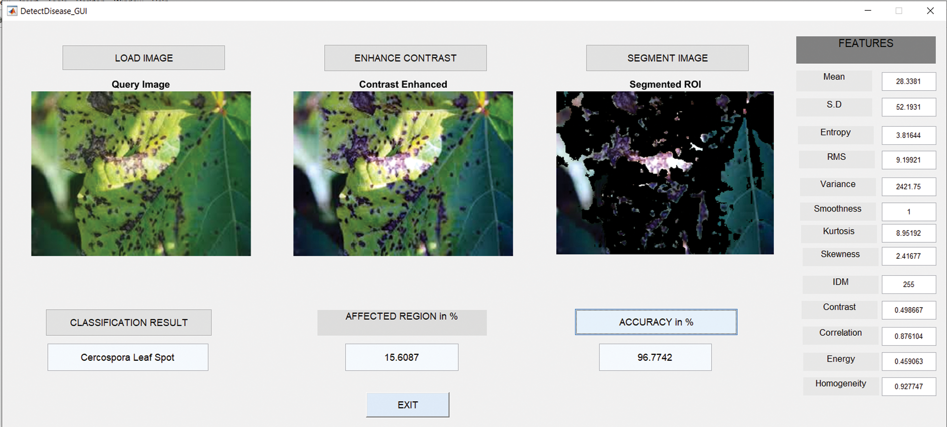
Figure 9: Cercospora leaf spot
6.5 Results in Case of Healthy Leaves
Fig. 10 shows the GUI of the proposed framework for the implemented scenario. In the case of Anthracnose, the accuracy obtained by the framework of about 98.39%.
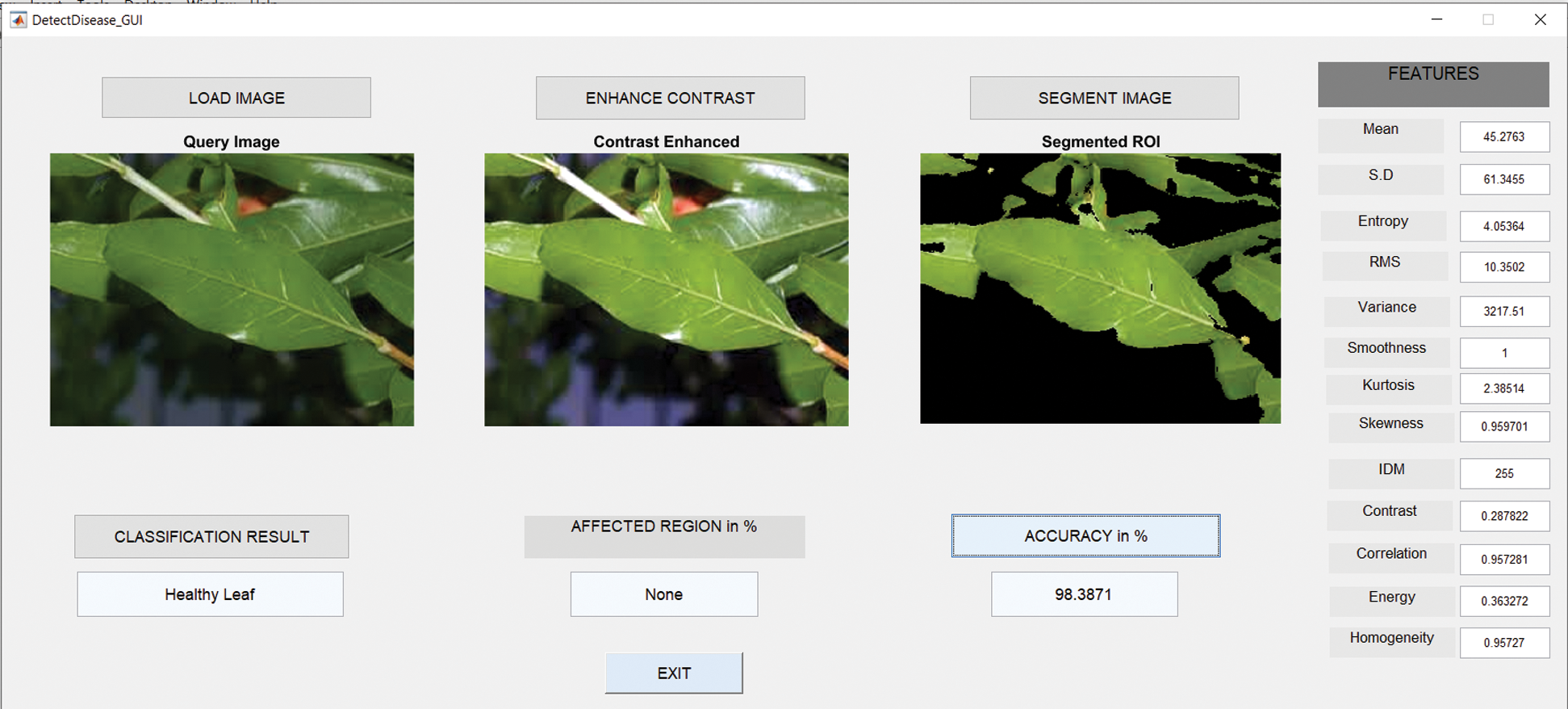
Figure 10: GUI for healthy leaf
The summary gives the accuracy of the designed model is about 98.39% in the case of Alternaria Alternata, Anthracnose, Bacterial Blast, and Healthy leaf. In the case of the Cercospora Leaf spot, accuracy is about 96.77%. The average accuracy is about 98.07%. A comparison of accuracy shown in Fig. 11. The accuracy achieved by another work with SVM [13] is 95.71%. The generated framework can achieve better accuracy of 98.07%. The complete details mentioned in Tab. 1.
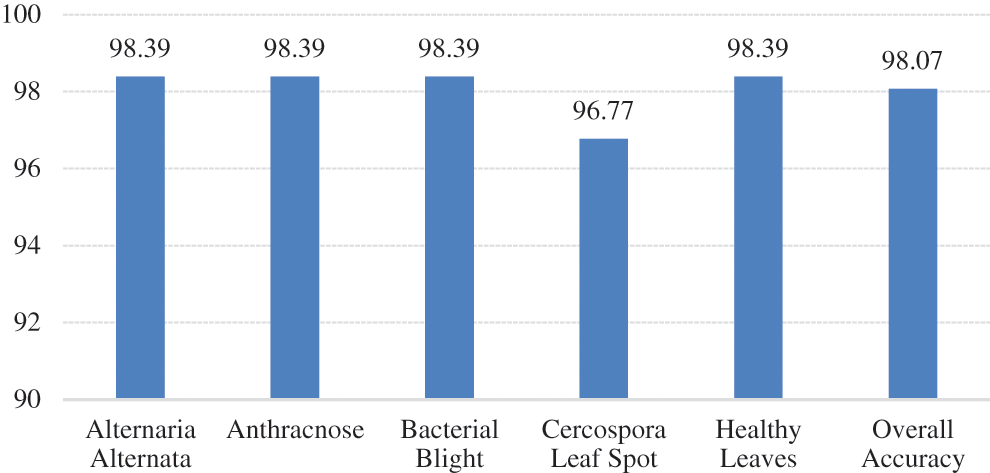
Figure 11: Comparison of accuracy across the classes and overall accuracy
Table 1: Summary of the evaluation metrics of the classification model
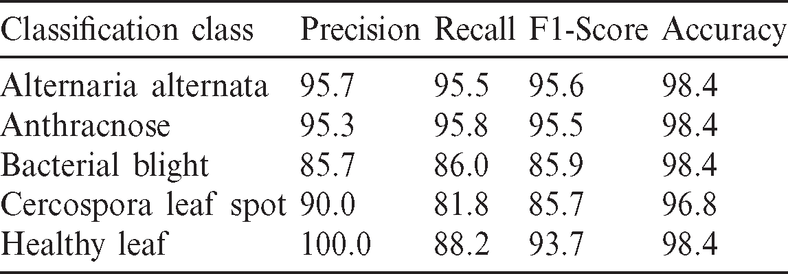
Besides the accuracy, other metrics such as precision, recall, and F1-score are also considered here. Accuracy carries misinformation if the data is unbalanced. To suppress that aspect, the additional metrics utilized to explain reliability. If the Precision and Recall metrics are closer to 1, i.e., closer to 100%, the corresponding F1-score will also be high, this situation implies the reliability of the generated classification model. The summary of all metrics presented in the Tab. 1. The graphical visualization of the evaluation metrics mentioned in Tab. 1 represented in Fig. 12.
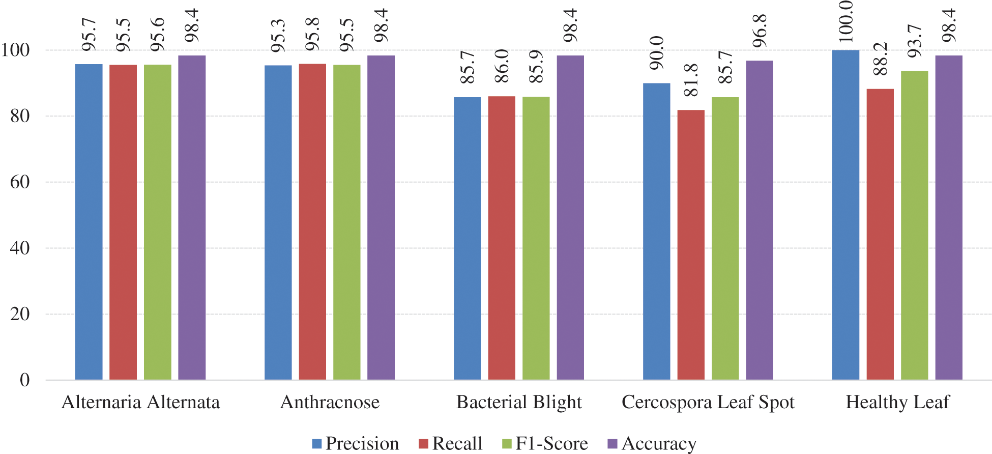
Figure 12: Graphical visualization of evaluation metrics of the model
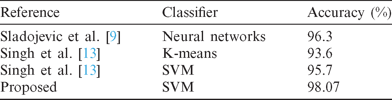
After validating the generated classification model with the help of various evaluation metrics such as accuracy, precision, recall, and F1-score, it is necessary to compare the current work with already published works for identifying which model can generate a better accuracy. The results presented in Tab. 2.
Table 2: Comparison of current work with published work
The article has presented a framework developed for the automatic identification and classification of pomegranate plant diseases based on the leaf images. The framework utilized advanced techniques such as image preprocessing, image segmentation, and image classification. Four kinds of diseases in pomegranate plants, such as Alternaria Alternata, Anthracnose, Bacterial Blight, and Cercospora Leaf Spot considered in the article. The designed framework can achieve an accuracy of about 98.39% across all categories except for Cercospora Leaf Spot. Overall accuracy across all the categories can achieve about 98.07%.
We have the plan to combine with deep learning to improve the accuracy of the framework in the future. If the framework can include a sufficient number of layers of CNN, it can get better accuracy.
Funding Statement: The author(s) received no specific funding for this study.
Conflicts of Interest: The authors declare that they have no conflicts of interest to report regarding the present study.
1 S. N. Ghaiwat and P. Arora. (2017). “Detection and classification of plant leaf diseases using image processing techniques: A review,” International Journal of Recent Advanced Engineering Technology, vol. 2, no. 3, pp. 2347–2353. [Google Scholar]
2 S. B. Dhaygude and N. P. Kumbhar. (2013). “Agricultural plant leaf disease detection using image processing,” International Journal of Advanced Research Electric Electron Instrumental Engineering, vol. 2, no. 1, pp. 11–22.
3 S. Arivazhagan, R. N. Shebiah, S. Ananthi and S. Vishnuvarthini. (2013). “Detection of an unhealthy region of plant leaves and classification of plant leaf diseases using texture features,” Agricultural Engineering International: CIGR, vol. 15, no. 1, pp. 211–217.
4 A. H. Kulkarni and A. R. K. Patil. (2012). “Applying image processing technique to detect,” International Journal of Modern Engineering and Research Technology, vol. 2, no. 5, pp. 3661–3664. [Google Scholar]
5 B. Sabah and N. Sharma. (2012). “Remote area plant disease detection using image processing,” International Organization of Scientific Research (IOSR) Journal of Electronics and Communications Engineering, vol. 2, no. 6, pp. 2278–2834. [Google Scholar]
6 D. Kaur and Y. Kaur. (2014). “Various image segmentation techniques: A review,” International Journal of Computer Science and Mobile Computing, vol. 3, no. 5, pp. 809–814. [Google Scholar]
7 S. Beucher and F. Meyer. (1993). “The morphological approach to segmentation: The watershed transforms,” in Mathematical Morphology in Image Processing, Washington, USA, Marcel Dekker Inc., vol. 12, pp. 433–481. [Google Scholar]
8 B. Bhanu and J. Peng. (2000). “Adaptive integrated image segmentation and object recognition,” Institute of Electrical and Electronics Engineers (IEEE) Transactions Systems, Man, Cybernetics, vol. 30, no. 5, pp. 421–441. [Google Scholar]
9 S. Sladojevic, M. Arsenovic, A. Anderla, D. Culibrk and D. Stefanovic. (2016). “Deep neural networks based recognition of plant diseases by leaf image classification,” Computational Intelligence and Neuroscience, vol. 2016, no. 1, pp. 1–18. [Google Scholar]
10 V. Singh, Varsha and A. K. Misra. (2015). “Detection of an unhealthy region of plant leaves using image processing and genetic algorithm,” in Proc. of Int. Conf. on Advanced Computer Engineering and Applications, vol. 1, no. 1, pp. 1028–1032. [Google Scholar]
11 S. D. Khirade and A. B. Patil. (2015). “Plant disease detection using image processing,” in Proc. of Int. Conf. on Computing Communication Control and Automation, vol. 153, no. 9, pp. 768–771. [Google Scholar]
12 E. Kiani and T. Mamedov. (2017). “Identification of plant disease infection using soft-computing: Application to modern botany,” Procedia Computer Science, vol. 120, no. 1, pp. 893–900. [Google Scholar]
13 V. Singh and A. K. Misra. (2017). “Detection of plant leaf diseases using image segmentation and soft computing techniques,” Information Processing Agriculture, vol. 4, no. 1, pp. 41–49. [Google Scholar]
14 K. Golhani, S. K. Balasundram, G. Vadamalai and B. Pradhan. (2018). “A review of neural networks in plant disease detection using hyperspectral data,” Information Processing in Agriculture, vol. 5, no. 3, pp. 354–371. [Google Scholar]
15 C. Mattihalli, E. Gedefaye, F. Endalamaw and A. Necho. (2018). “Plant leaf disease detection and auto-medicine,” Internet of Things, vol. 1, no. 2, pp. 67–73. [Google Scholar]
16 X. E. Pantazi, D. Moshou and A. A. Tamouridou. (2018). “Automated leaf disease detection in different crop species through image features analysis and one-class classifiers,” Computers and Electronics in Agriculture, vol. 156, no. 5, pp. 96–104. [Google Scholar]
17 S. Sankaran, A. Mishra, R. Ehsani and C. Davis. (2010). “A review of advanced techniques for detecting plant diseases,” Computers and Electronics in Agriculture, vol. 72, no. 1, pp. 1–13. [Google Scholar]
18 K. P. Ferentinos. (2018). “Deep learning models for plant disease detection and diagnosis,” Computers and Electronics in Agriculture, vol. 145, no. 4, pp. 311–318. [Google Scholar]
 | This work is licensed under a Creative Commons Attribution 4.0 International License, which permits unrestricted use, distribution, and reproduction in any medium, provided the original work is properly cited. |