DOI:10.32604/cmc.2020.014220

| Computers, Materials & Continua DOI:10.32604/cmc.2020.014220 |  |
| Article |
3D Reconstruction for Motion Blurred Images Using Deep Learning-Based Intelligent Systems
1Tamoritsusho Co., Ltd., Tokyo, 110-0005, Japan
2Department of Computer Science and Technology, Xi’an University of Science and Technology, Xi’an, 710054, China
3Global Information and Telecommunication Institute, Waseda University, Tokyo, 169-8050, Japan
4School of Fundamental Science and Engineering, Waseda University, Tokyo, 169-8050, Japan
5Department of Electronics and Communications Engineering, East West University, Dhaka, 1212, Bangladesh
*Corresponding Author: Keping Yu. Email: keping.yu@aoni.waseda.jp
Received: 07 September 2020; Accepted: 11 October 2020
Abstract: The 3D reconstruction using deep learning-based intelligent systems can provide great help for measuring an individual’s height and shape quickly and accurately through 2D motion-blurred images. Generally, during the acquisition of images in real-time, motion blur, caused by camera shaking or human motion, appears. Deep learning-based intelligent control applied in vision can help us solve the problem. To this end, we propose a 3D reconstruction method for motion-blurred images using deep learning. First, we develop a BF-WGAN algorithm that combines the bilateral filtering (BF) denoising theory with a Wasserstein generative adversarial network (WGAN) to remove motion blur. The bilateral filter denoising algorithm is used to remove the noise and to retain the details of the blurred image. Then, the blurred image and the corresponding sharp image are input into the WGAN. This algorithm distinguishes the motion-blurred image from the corresponding sharp image according to the WGAN loss and perceptual loss functions. Next, we use the deblurred images generated by the BF-WGAN algorithm for 3D reconstruction. We propose a threshold optimization random sample consensus (TO-RANSAC) algorithm that can remove the wrong relationship between two views in the 3D reconstructed model relatively accurately. Compared with the traditional RANSAC algorithm, the TO-RANSAC algorithm can adjust the threshold adaptively, which improves the accuracy of the 3D reconstruction results. The experimental results show that our BF-WGAN algorithm has a better deblurring effect and higher efficiency than do other representative algorithms. In addition, the TO-RANSAC algorithm yields a calculation accuracy considerably higher than that of the traditional RANSAC algorithm.
Keywords: 3D reconstruction; motion blurring; deep learning; intelligent systems; bilateral filtering; random sample consensus
Due to some factors, such as camera shaking and human motion, real-time image blurring easily occurs. For a good visual effect, it is very important to remove the blur and obtain a sharp image [1]. The “intelligent” solutions are essential in solving the blurring problem by using the effective critical thinking procedures to restore the sharp image. Most of the existing image deblurring methods are based on the image prior probability model. Krishnan et al. [2] assumed that the image gradient obeys the Laplace distribution, and Zoran et al. [3] simulated the distribution of the image gradient with a Gaussian mixture model. The image prior probability methods overlap with noise in the frequency domain or transform domain, so the excessive smoothing of texture structures greatly reduces the visual effect. In recent years, many scholars have applied deep learning to image deblurring algorithms. Xu et al. [4] proposed an image deblurring method based on a convolutional neural network (CNN) to overcome the ringing effect in saturated regions of images. Chakrabarti [5] predicted complex Fourier coefficients of motion kernels to perform non-blind deblurring in the Fourier space. Gong et al. [6] used a fully convolutional network for motion flow estimation. Nah et al. [7] adopted a kernel-free end-to-end approach that uses a multiscale CNN to directly deblur the image. However, the CNN method considers the prior features of the image indirectly, which are easily affected by noise.
To solve the problems of the existing deep learning algorithms, we propose a BF-WGAN algorithm, which combines the bilateral filtering (BF) [8] denoising theory with the Wasserstein generative adversarial network [9] (WGAN), to remove motion-blurred images. The BF-WGAN algorithm contains two parts. First, the bilateral filter denoising algorithm is used to remove the noise and retain the details of the blurred image. The advantage of the bilateral filter theory is that it not only considers the spatial distance between pixels but also considers the degree of similarity between pixels, which ensures that the pixel values near the edge are preserved. Second, the blurred image and corresponding sharp image are input into the WGAN. This algorithm distinguishes the motion-blurred image from the corresponding sharp image according to the WGAN loss and perceptual loss [10] functions, which allows the finer texture-related details to be restored and the high-precision contours of the image to be revealed. Further, the BF-WGAN has fewer parameters comparing to multiscale CNN, which heavily speeds up the inference. Therefore, the BF-WGAN obtain state-of-the-art results in motion deblurring while faster than the closest competitor-CNN.
3D reconstruction of the human body is very useful for the rapid and accurate measurement of an individual’s height and body shape [11]. With the use of 2D real-time images of the human body taken from different angles, 3D reconstruction technology can quickly and accurately provide information on the growth of children. At present, it is estimated that there are approximately 149 million children under the age of 6 with physical dysplasia worldwide. A child’s height and shape can directly reflect his or her magnitude of growth [12]. Because there are many children that need to be evaluated, the traditional manual measurement methods for height and body shape require considerable manpower and time.
For the 3D reconstruction of motion-blurred images, we use the deblurred images generated with the BF-WGAN algorithm to perform the 3D reconstruction. The most important part of 3D reconstruction is the calculation of the camera parameters, which mainly include the global rotation matrix and global translation vector for multiview 3D reconstruction [13]. The global rotation matrix was used to remove the wrong relationship between two views in the 3D reconstructed model. A commonly used method to calculate the global rotation matrix is the RANSAC algorithm [14]. However, the traditional RANSAC algorithm uses a fixed threshold, which can affect the accuracy of the global rotation matrix. This paper proposes a threshold optimization random sample consensus (TO-RANSAC) algorithm that can adjust the threshold adaptively to improve the accuracy of the 3D reconstruction results.
The contributions of this paper are listed as follows:
a) We use deep learning-based intelligent systems to remove the motion blur in images. The BF-WGAN algorithm is proposed, which combines the BF denoising theory with WGAN. The BF denoising algorithm is used to remove the noise and retain the details of the blurred image. The WGAN adopts the blurred image, and corresponding sharp images are input into the WGAN. The BF-WGAN algorithm has a better deblurring effect and higher efficiency than other representative algorithms.
b) We adopt the deblurred images generated from the BF-WGAN algorithm to perform the 3D reconstruction. The TO-RANSAC algorithm is proposed, which can remove the wrong relationship between two views in the 3D reconstructed model relatively accurately. Compared with the traditional RANSAC algorithm, the TO-RANSAC algorithm can adjust the threshold adaptively, which improves the accuracy of the 3D reconstruction results.
The remainder of this paper is organized as follows: Section 2 consists of two parts. Part 2.1 presents the deep learning-based intelligent systems to remove the motion blur of images through the BF-WGAN algorithm, and Part 2.2 explains the TO-RANSAC algorithm that we used to perform the 3D reconstruction. In Section 3, we designed and evaluated an experiment to test the performance of the BF-WGAN algorithm and the TO-RANSAC algorithm. In Section 4, we conclude our study and suggest directions for future work.
Normally, the processing of an image depends upon the quality, and the captured image in poor quality might result in a mistake. The intelligent systems using intelligent decision-making algorithms and techniques can help us to solve the image blurring problem.
In a mathematical model, image blurring can be described by the convolution process for an image. The original sharp image  is convolved with the blurring kernel
  , while noise
  is added. Then, we obtain the blurred image [15]:

where  is a convolution operator.
2.1.1 Bilateral Filter Denoising Algorithm
A bilateral filter is a nonlinear denoising algorithm that eliminates noise while preserving image details [16]. The general Gaussian filter mainly considers the spatial distance between pixels when sampling but does not consider the degree of similarity between pixels [17]. Compared with the Gaussian filter, the bilateral filter considers both the spatial distance and degree of similarity, thereby suppressing the irrelevant details and enhancing the sharp edges of the image.
Step 1: Compute the Gaussian weight region filter based on the spatial distances:

where  and
and  represent the input image and output image, respectively.
  is near the neighborhood centered on
  .
.  is the Gaussian weight based on spatial distance, which is used to measure the spatial distance between the center
  and the point
  .
.

where  ,
,  is the standard deviation.
  is the normalization factor:

Step 2: Obtain the edge filter based on the degree of similarity:

where  is the weight based on the degree of similarity between pixels:

where  ,
,  is the standard deviation.
  is the normalization factor:

Step 3: Create the bilateral filter by combining the Gaussian weight region filter with the edge filter:

where  is the normalization factor:

After the local subregion  is defined, the discretized form of the formula (8) can be expressed as follows:

2.1.2 WGAN Deblurring Algorithm
This paper proposes a WGAN deblurring algorithm that adopts both the WGAN loss and perceptual loss functions [18]. The WGAN loss function ensures that the generated samples are diverse, thereby allows the fine texture-related details to be restored. The input and output results of the WGAN deblurring algorithm are shown in Fig. 1. The input is the motion-blurred image, and the output result is the deblurred image [19].
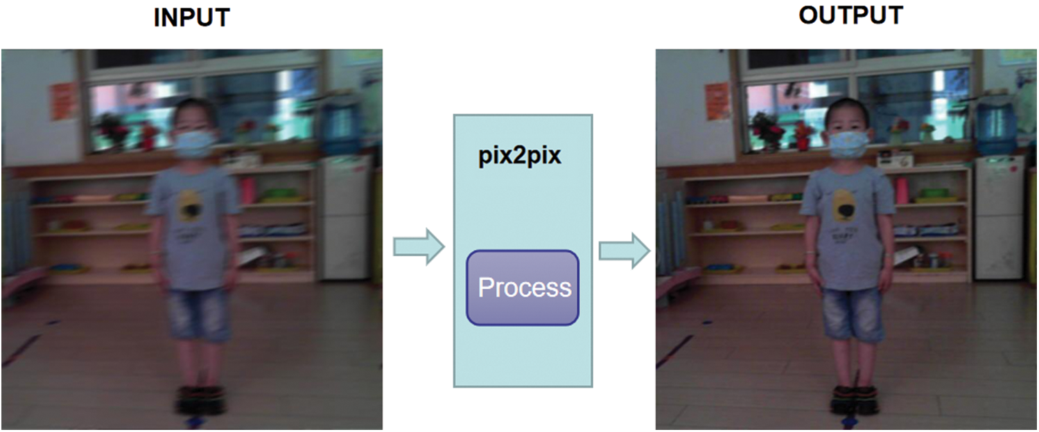
Figure 1: Input and output results of the WGAN deblurring algorithm
The WGAN between generator  and discriminator
  is the minimax value using Kantorovich-Rubinstein duality [20]:

where  represents the original sharp image and
  represents the expectation.
  is the set of 1-Lipschitz functions.
  is the data distribution, and
  is the model distribution, defined by
  , where the input
  represents the blurred image.
  represents the probability that
  is a real image.
① WGAN framework
As shown in Fig. 2, the framework of the WGAN deblurring algorithm consists of a generator and a discriminator [21].
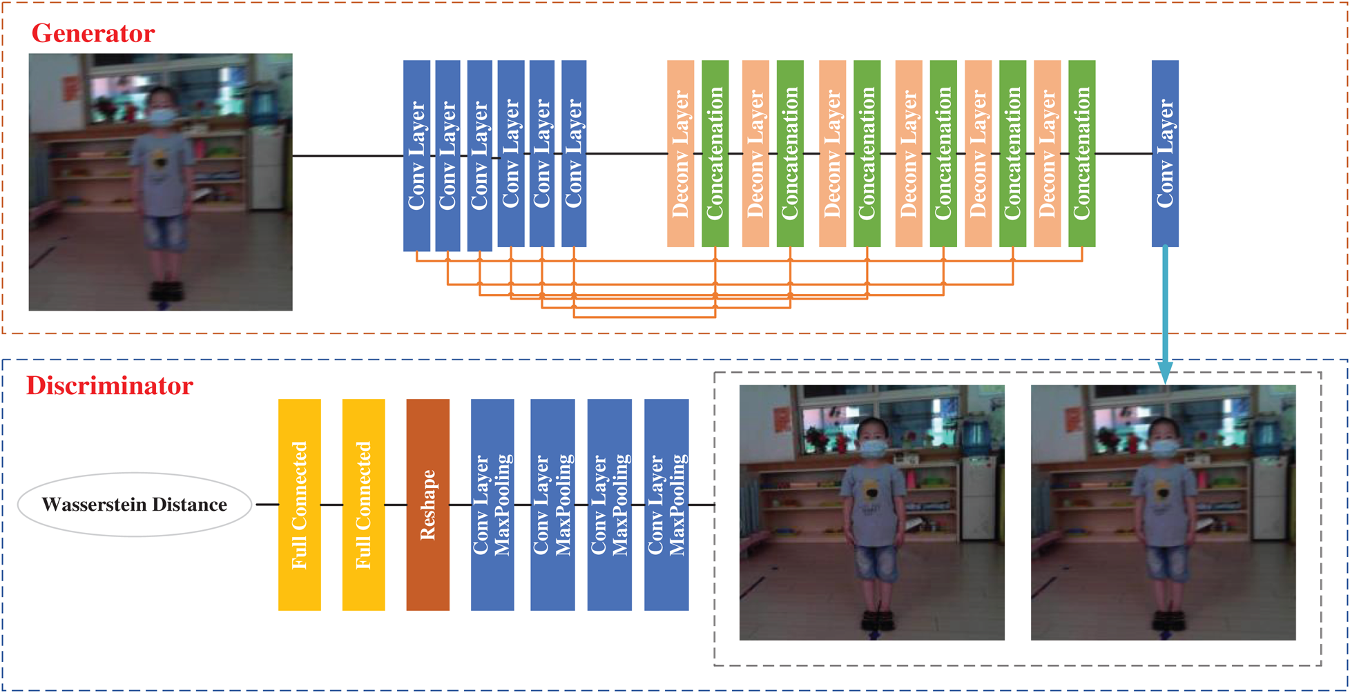
Figure 2: Framework of the WGAN deblurring algorithm
② Loss Function
The loss function of this paper consists of the WGAN loss and perceptual loss functions. The total loss function  is defined as follows:

where  and is set according to the experience value.
WGAN loss. The WGAN loss  is calculated as follows:

where  represents the blurred image. Deblurring is performed by the trained generator
  and discriminator
  .
.  represents the size of the training data [22].
Perceptual loss. The perceptual loss function is defined as follows:

where  and
and  are the dimensions of the feature maps.
  is the feature map obtained by the j-th convolution before the i-th maxpooling layer within the VGG19 network [23].
  represents the sharp image, and
  represents the blurred image.
2.2 Multi-view 3D Reconstruction Based on the TO-RANSAC Algorithm
Multiview 3D reconstruction is mainly composed of four parts: (1) Feature extraction and matching; (2) Camera parameter calculation; (3) 3D point cloud calculation; and (4) Bundle adjustment. The camera parameter calculation mainly involves the global rotation matrix and global translation vector for multiview 3D reconstruction [24]. The global rotation matrix is used to remove the wrong relationship between two views in the 3D reconstructed model.
The most commonly used method to calculate the global rotation matrix is the RANSAC algorithm [25]. However, the traditional RANSAC algorithm adopts a fixed threshold, which can affect the accuracy of the global rotation matrix. To improve the calculation accuracy, a threshold optimization random sample consensus algorithm (TO-RANSAC) is proposed. The TO-RANSAC algorithm can adjust the threshold adaptively, which prevents errors caused by different thresholds in the 3D reconstruction results.
The global rotation matrix is calculated by the relative rotation matrix through the least-squares optimization algorithm. The formula is shown in (15):

where  is a known relative rotation matrix,
  and
and  are two global rotation matrices that need to be calculated respectively. First, we calculate the global rotation matrices. The wrong relationship between two views needs to be removed. Then, the global rotation matrices can be calculated with the formula (15).
This paper proposes a TO-RANSAC algorithm to remove the wrong relationship between two views in the 3D reconstructed model. TO-RANSAC is a combination of the RANSAC algorithm and the threshold optimization concept. The use of different threshold parameters for the traditional RANSAC will affect the algorithm results. To avoid this problem, the TO-RANSAC algorithm is used to determine whether the model is reliable on the basis of the  (number of false alarms) value [26]. Generally, the smaller the value of
  , the more reliable the model is. The calculation formula is:

where  is the calculated model parameter,
  is the number of assumed correct samples,
  is the number of possible models,
  is the number of total samples,
  is the minimum number of samples used to generate the model
  ,
,  is the k-th smallest error for the model
  , and
, and  is the probability that the random error is 1.
The flow chart of the TO-RANSAC algorithm is shown in Fig. 3. The TO-RANSAC algorithm consists of five steps, which are expressed below:
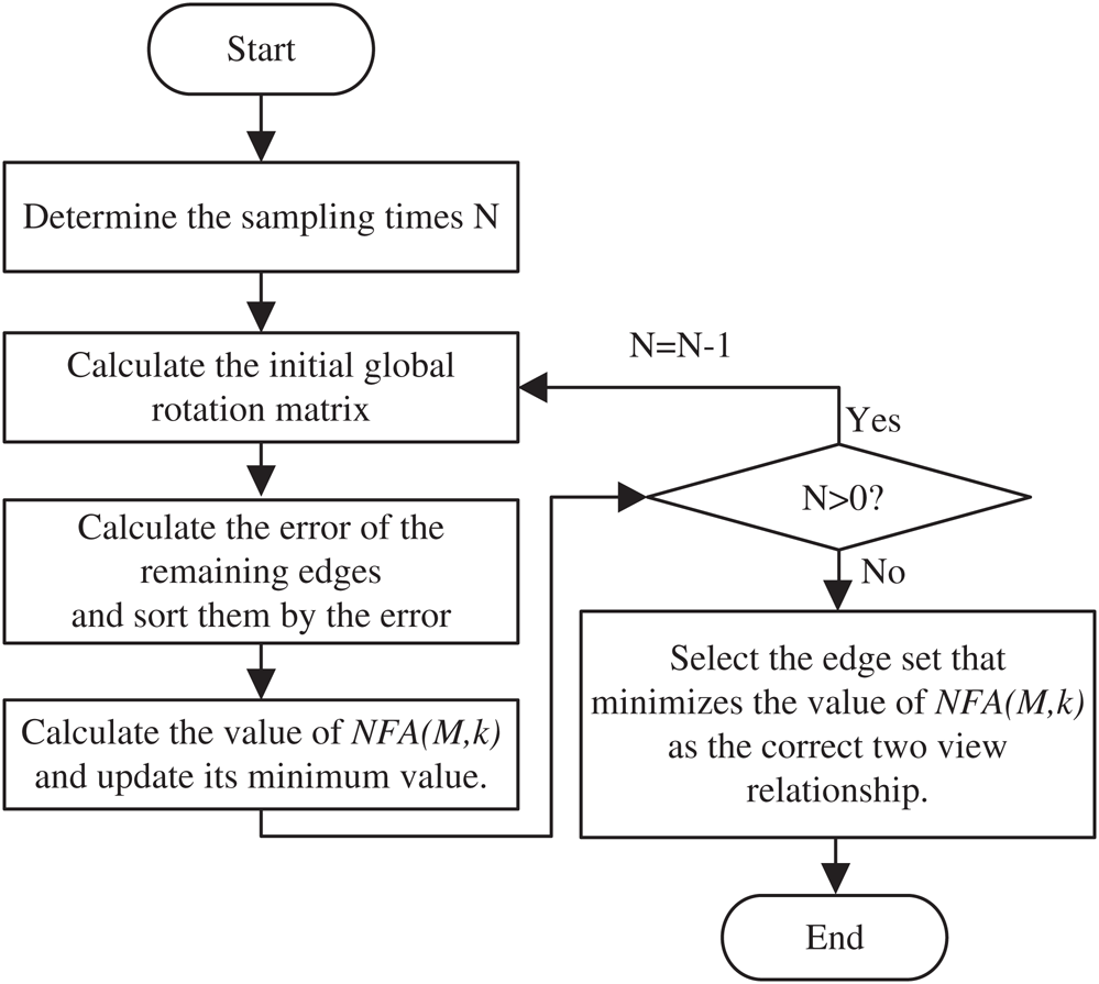
Figure 3: Flow-chart of the TO-RANSAC algorithm
Step 1: Determine the sampling times  . We used formula (17) to determine the sampling times
  .
.
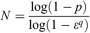
where  is the confidence value, which was set to be
  .
.  represents the minimum number of samples required for the calculation model, which was set to be
  .
.  is the interior point rate, which was set to be
  .
.
Step 2: Calculate the initial global rotation matrix. Formula (16) is used, where  represents the initial global rotation matrix, which is calculated by the random spanning tree;
  is the number of all two-view relationships, and
  is the number of edges on the random spanning tree.
Step 3: Calculate the errors for the remaining edges and sort the edges by the magnitude of the error. The error was calculated as the angle difference between the relative rotation matrix and the global rotation matrix, and the formula used is:

In formula (18),  is the angle between the vectors
  and
and  .
.
Step 4: Calculate the value of  and update its minimum value. If
  , the algorithm returns to step 2, and the sampling times
  are reduced by 1; otherwise, the algorithm proceeds to Step 5.
Step 5: Select the edge set that minimizes the value of  according to the correct two-view relationship.
For the performance evaluation of our approach, we collected 3000 real-time images of children from a kindergarten. There were 100 children aged 2–6 years, including 50 female students and 50 male students. A total of 30 real-time images were collected for each student in the JPG format. To evaluate the effect of the 3D reconstruction method for motion-blurred images, we simulated the method in three parts. First, simulated noise images and blurred images were generated. The noise images and blurred images were generated by a ThinkPad S3-490 computer [27]. The algorithms for the simulated noise images and blurred images were run by MATLAB 2018b. Second, the BF-WGAN algorithm was run on GeForce RTX 2080Ti GPU and executed with Python. Moreover, the TO-RANSAC algorithm was run on a ThinkPad S3-490 computer for deblurring images, which was executed by MATLAB 2018b.
The children were aged from 2–6 years, and one student of each age was selected as an example. Fig. 4 shows the original sharp images of five students from five different angles. The first child was a boy who was 2 years old, and his height was 80.3 cm. The second child was a girl who was 3 years old, and her height was 92.4 cm. The third child was a girl who was 4 years old, and her height was 101.7 cm. The fourth child was a girl who was 5 years old, and her height was 112.3 cm. The fifth child was a boy who was 6 years old, and his height was 123.1 cm. The size of the original sharp images was 512 × 512 pixels.
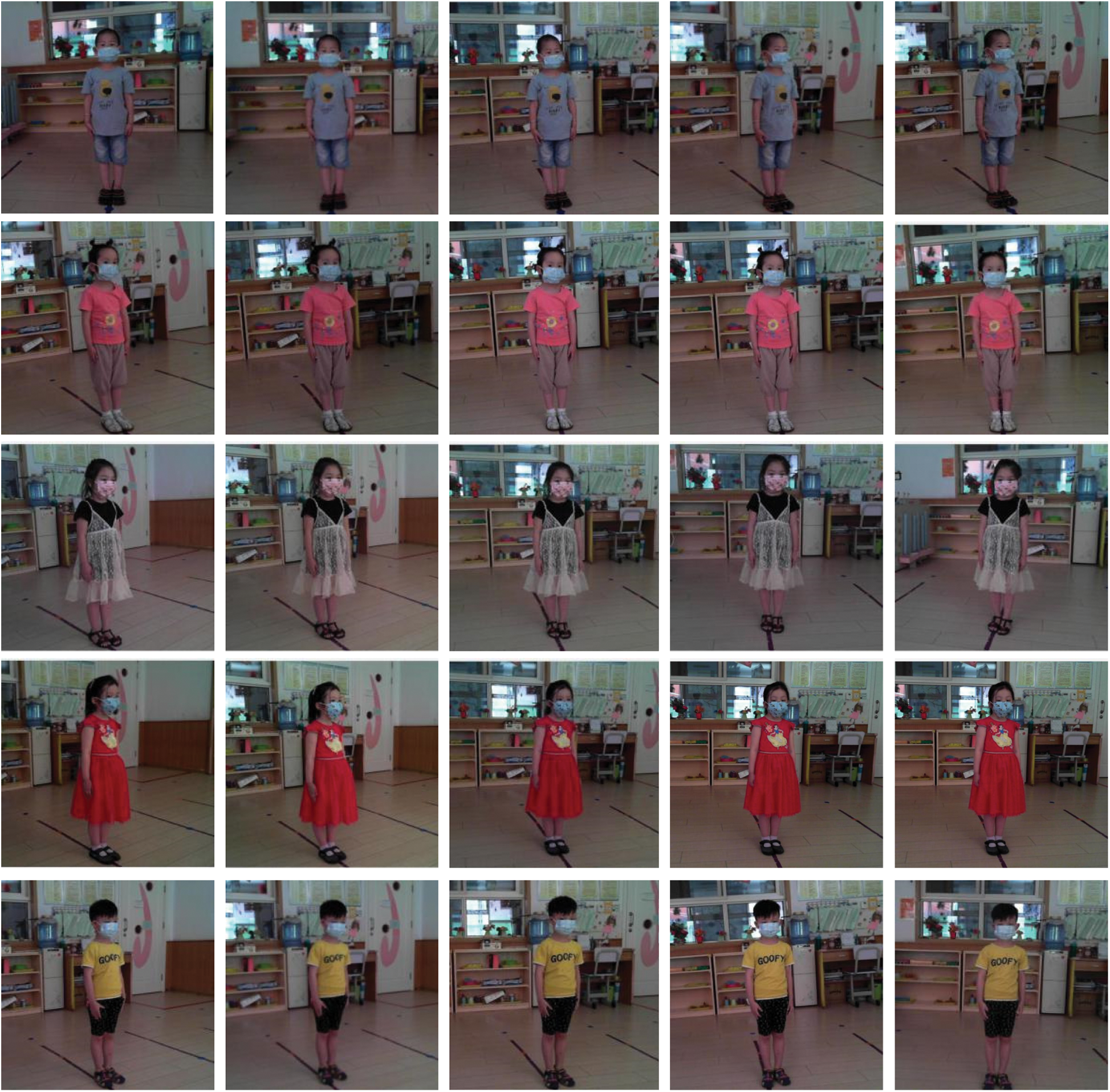
Figure 4: Original sharp images of five students
3.1 Generation of Simulated Noise and Blurred Images
We chose the images of a 2-year-old boy and a 4-year-old girl to simulate the experiment. For the generation of simulated noise and blurred images, we mainly considered two aspects: the image noise parameters and motion blur parameters.
Gaussian noise is a common type of noise that occurs with camera shaking [28]. The MATLAB library includes a function that adds noise to an image, the imnoise function. We used the imnoise function to add Gaussian noise to the image. Fig. 5 shows the Gaussian noise image with variances  ,
,  and
and  .
.
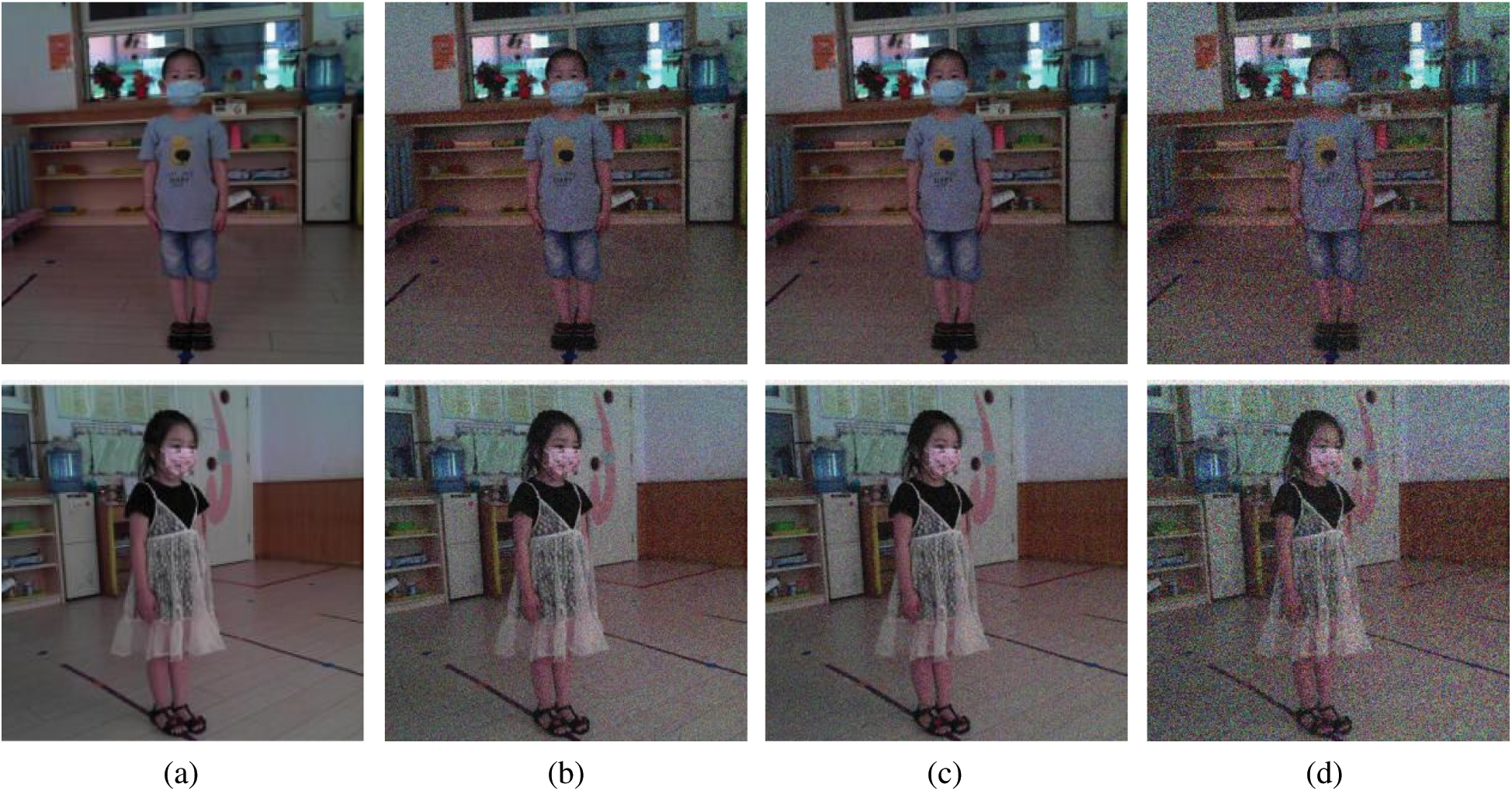
Figure 5: Gaussian noise image with different variances. (a) original sharp image. (b)  . (c)
. (c)  . (d)
. (d) 
We used the MATLAB special function to blur the image and mainly considered two aspects: The blur angle and blur amplitude. For the blur angle, the blur amplitude was set to 15 pixels, and the blur angles studied were 30°, 45°, and 60°. Fig. 6 shows the generated images of the two students with different blur angles and blur amplitudes.
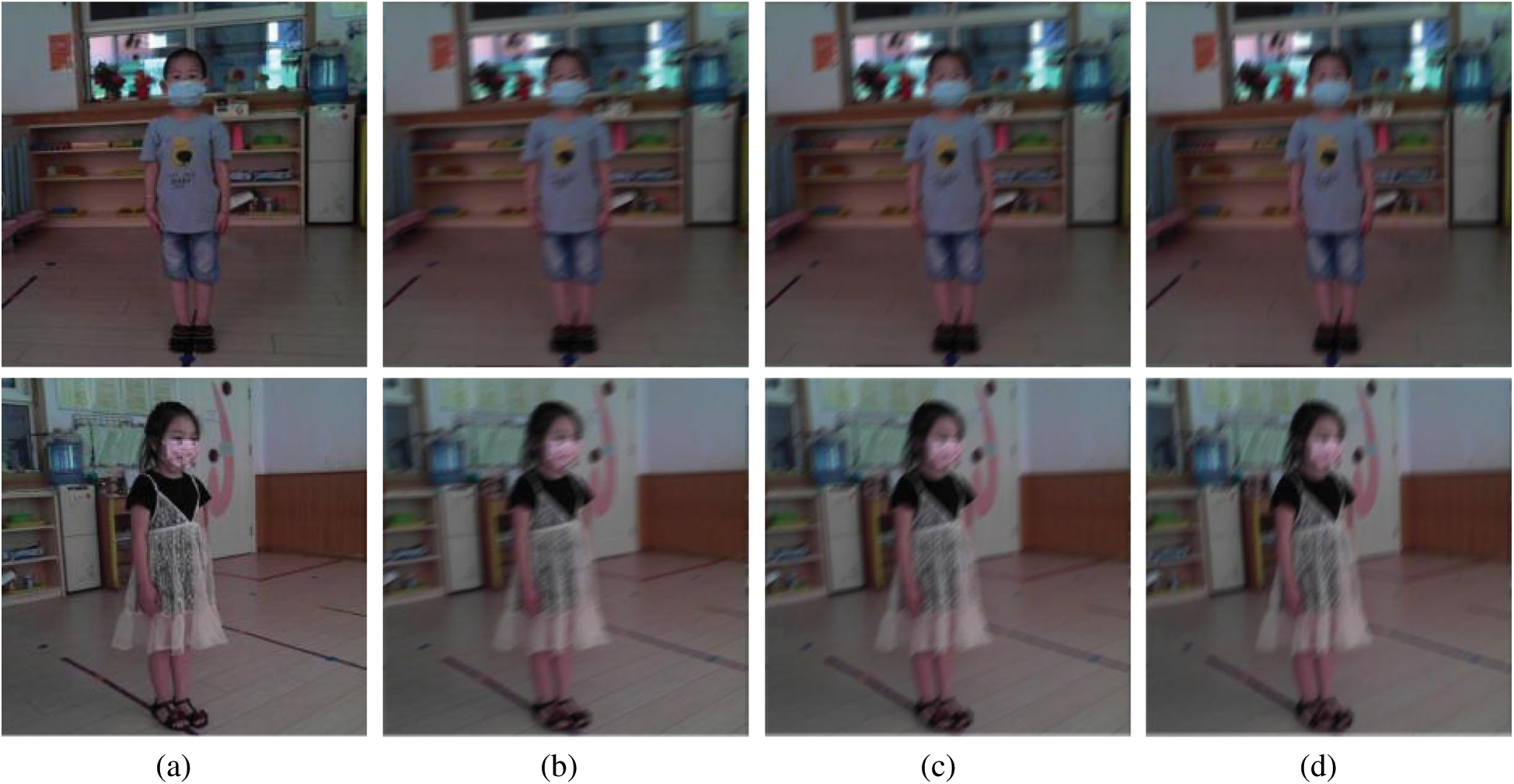
Figure 6: Images of the two students with different blur angles. (a) Original sharp image. (b) Blur angle of 30°. (c) Blur angle of 45°. (d) Blur angle of 60°
3.2 Experiment of BF-WGAN Algorithm
Fig. 7 shows the image restoration results with noise and blurred image. Set the image restoration results with Gaussian noise variance  , and the image restoration results with a blur amplitude of 15 pixels and a blur angle of
  . Fig. 7 shows that BF-WGAN algorithm effectively removes the noise and restores the fine texture-related details.
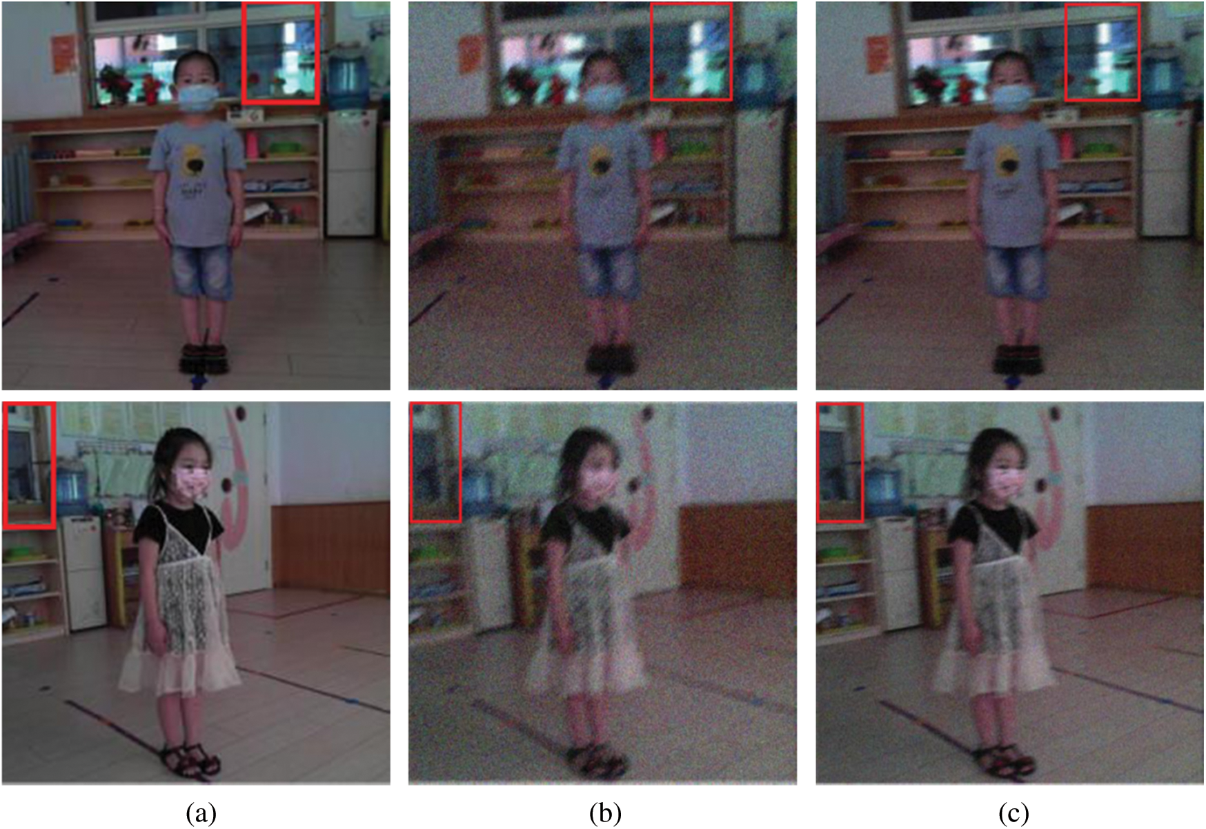
Figure 7: Image restoration results with noise and blurred images. (a) Original sharp image. (b) Noise and blurred image. (c) Restored image
For comparison, we compared our algorithm with other image deblurring algorithms, including Xu L’s algorithm [6], Chakrabarti A’s algorithm [7], Gong D’s algorithm [8] and Nah S’s algorithm [9]. Figs. 8 and 9 show the results of the comparison of the different algorithms, including the noise and blurred images of two students. (a) is the original sharp image. (b) shows the images with Gaussian noise variance  , with a blur amplitude of 20 pixels and a blur angle of 60°. (c) is the image restored with our BF-WGAN algorithm. (d) is the image restored with Xu L’s algorithm. (e) is the image restored with Chakrabarti A’s algorithm. (f) is the image restored with Gong D’s algorithm. (g) is the image restored with Nah S’ s algorithm. Compared with the other four algorithms, our algorithms yielded the largest degree of restoration of the edge blur of the image, and the resulting image was the most similar to the original sharp image.
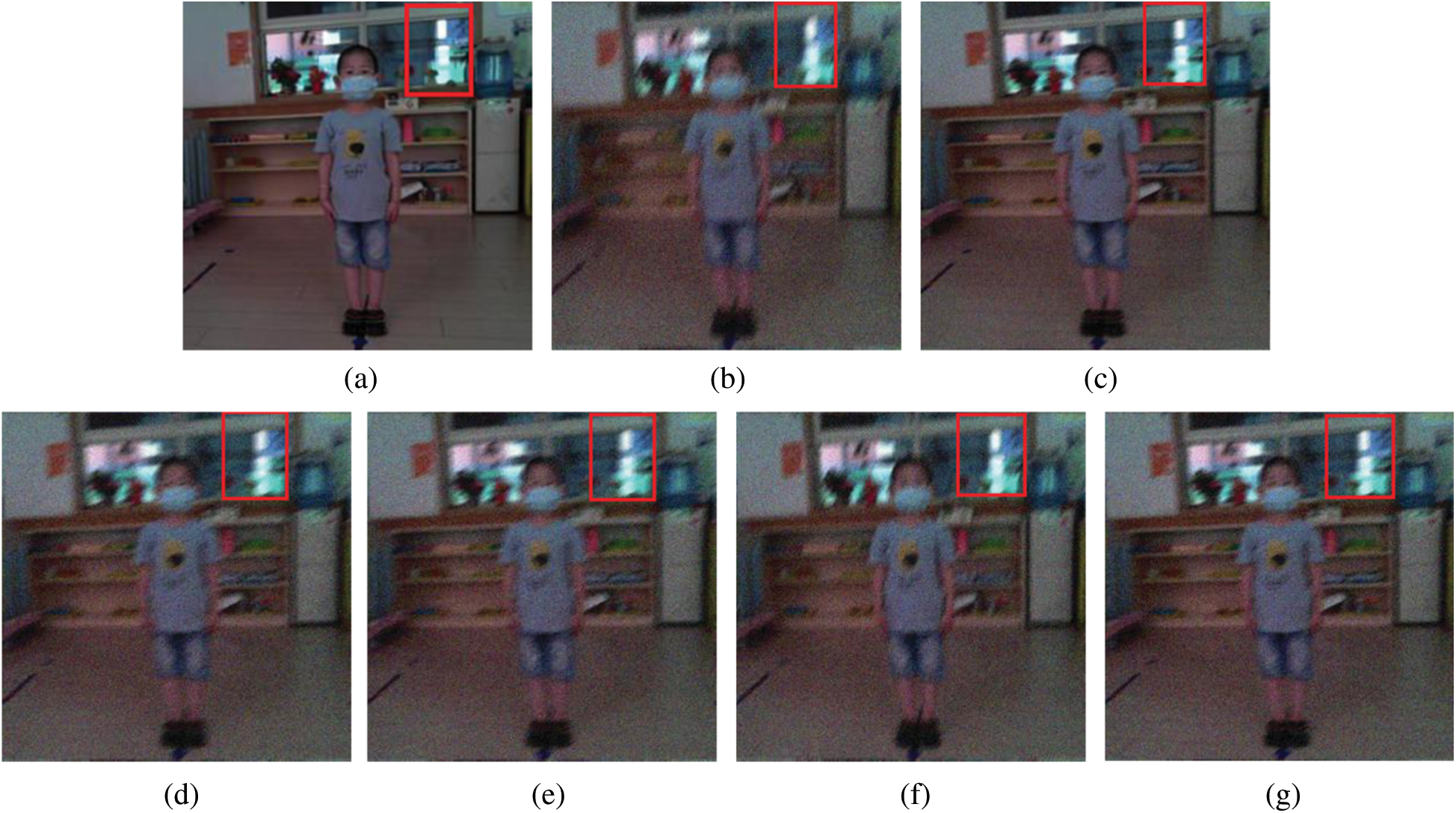
Figure 8: Image restoration results with various algorithms for a male student. (a) Original sharp image. (b) Noise and Blurred image. (c) BF-WGAN approach. (d) Xu L’s algorithm. (e) Chakrabarti A’s algorithm. (f) Gong D’s algorithm. (g) Nah S’s algorithm
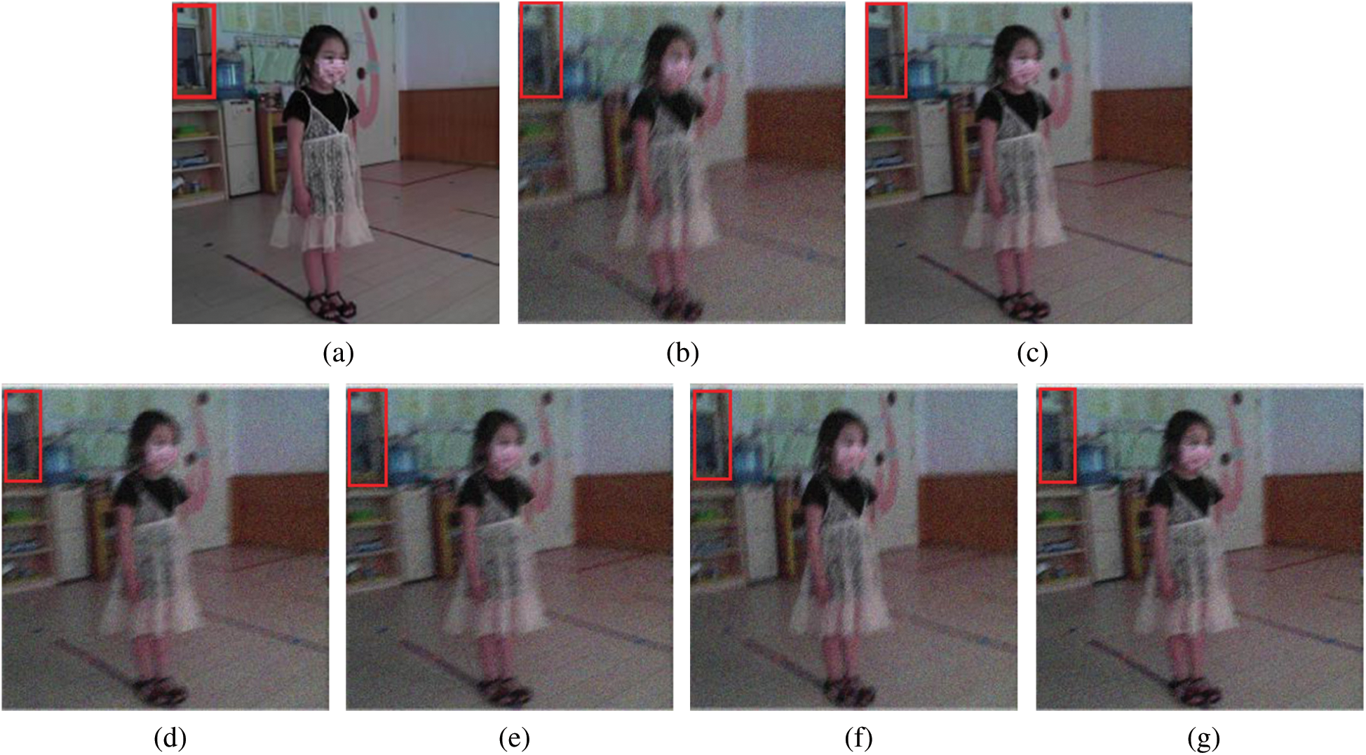
Figure 9: Image restoration results with various algorithms for a female student. (a) Original sharp image. (b) Noise and Blurred image (c) BF-WGAN approach. (d) Xu L’s algorithm. (e) Chakrabarti A’s algorithm. (f) Gong D’s algorithm. (g) Nah S’s algorithm
① Time Contrast Experiment
For the time contrast experiment of image deblurring, the images of a 2-year-old boy and a 4-year-old girl were selected. The experiment was repeated 3 times for each group, and then, the average value of three measurements was used for analysis.
Tab. 1 shows the time contrast results of image deblurring using five algorithms. The BF-WGAN algorithm greatly reduces the time required for image deblurring because the BF-WGAN algorithm has fewer parameters than does the CNN, which greatly speeds up the inference process.
Table 1: Comparison of the time required for image deblurring using five algorithms

② Accuracy Contrast Experiment
We adopt the peak signal-to-noise ratio (PSNR) [29,30] to measure the accuracy of image deblurring. For the blurred image of the 2-year-old boy, the images had Gaussian noise variance  , a blur amplitude of 20 pixels, and blur angle of
  . Figs. 10 and 11 show the PSNR results of the blurred image for the five algorithms. The PSNR value of our BF-WGAN is higher than the other four representative algorithms, and it yields a better restoration effect.
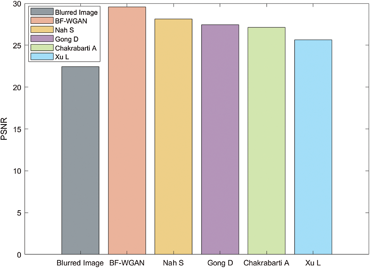
Figure 10: Comparison of the PSNR value for a 2-year-old boy
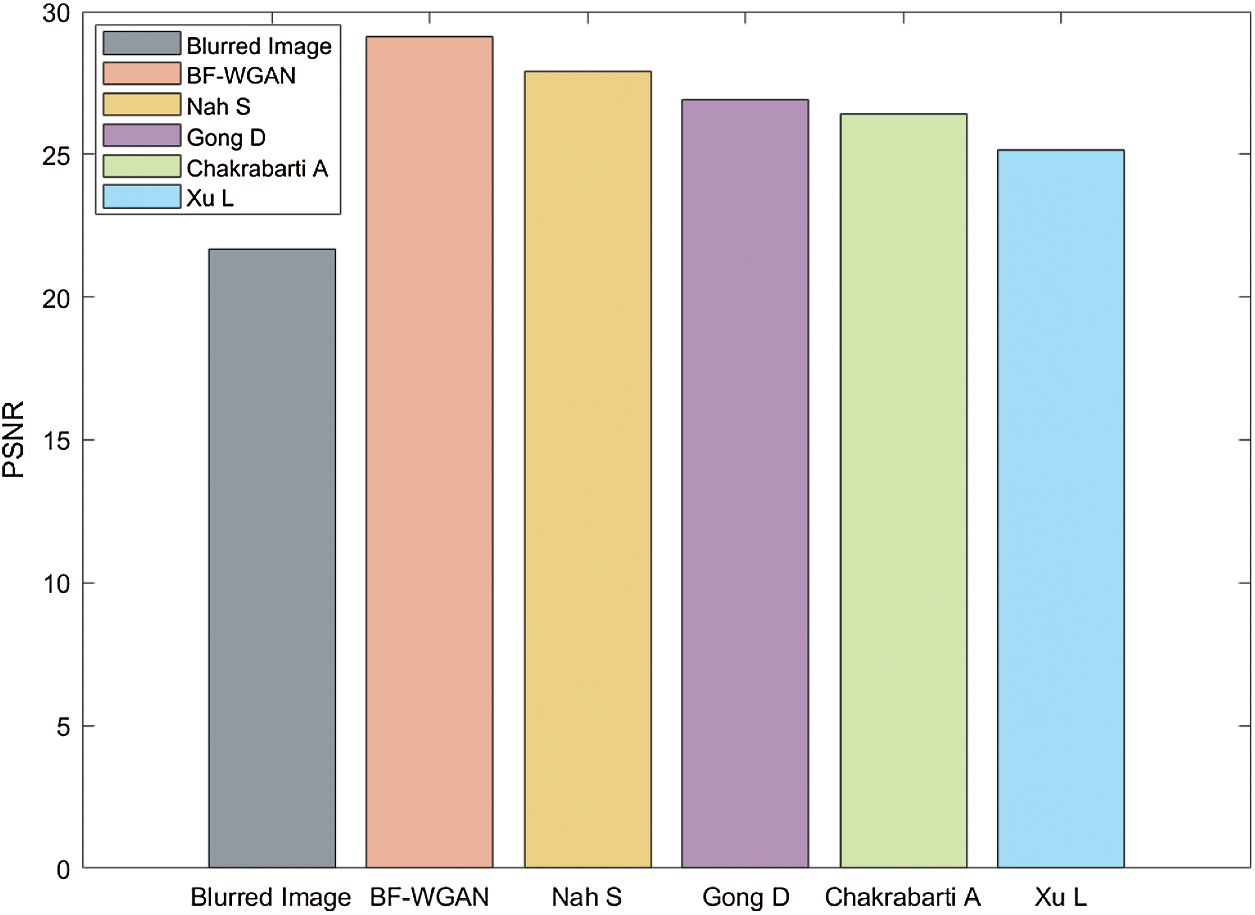
Figure 11: Comparison of the PSNR value for a 4-year-old girl
3.3 Experiment of 3D Reconstruction
3.3.1 Results of 3D Reconstruction
Fig. 12 shows the 3D reconstruction results for the 2-year-old boy. According to the 3D reconstruction results, the height, shoulder width and head width of the 2-year-old boy were 79.1 cm, 25.3 cm and 14.2 cm, respectively. Compared with the actual measured data of the 2-year-old boy, the differences in the height, shoulder width and head width were 1.2 cm, 0.7 cm and 0.5 cm, respectively. Therefore, the AC-RANSAC 3D reconstruction algorithm presents a reasonable reconstruction effect.
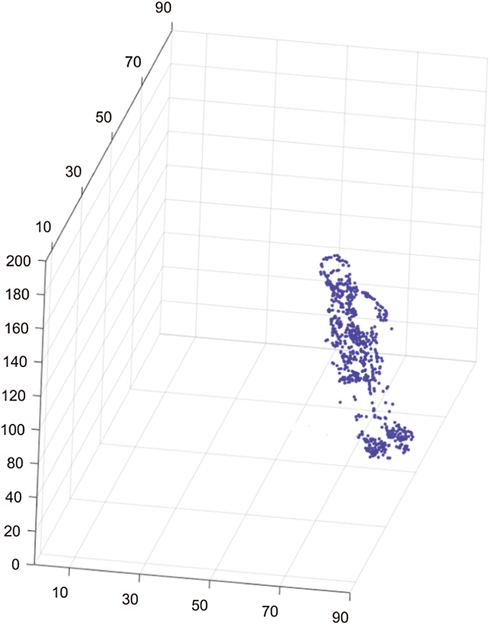
Figure 12: 3D reconstruction results for the 2-year-old boy
Fig. 13 shows the 3D reconstruction results for the 4-year-old girl. According to the 3D reconstruction results, the height, shoulder width and head width of the 4-year-old girl were 102.5 cm, 28.7 cm and 17.2 cm, respectively. Compared with the actual measured data of the 2-year-old boy, the differences in the height, shoulder width and head width were 0.8 cm, 0.6 cm and 0.4 cm, respectively. Therefore, the AC-RANSAC 3D reconstruction algorithm also presents a reasonable reconstruction effect.
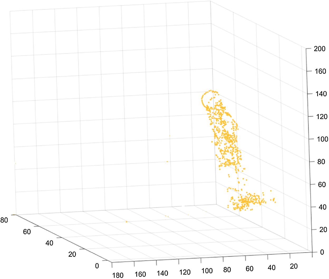
Figure 13: 3D reconstruction results for the 4-year-old girl
3.3.2 Performance of 3D Reconstruction
The TO-RANSAC and RANSAC algorithms were used to remove the wrong two-view relationships. For the 2-year-old boy and 4-year-old girl, Tabs. 2 and 3 show the comparison of the wrong edges removed with the TO-RANSAC and RANSAC algorithms. The threshold parameter of the RANSAC was set to 1°, and the TO-RANSAC algorithm used the adaptive threshold parameters. The second column in the table shows the number of wrong edges removed after using the TO-RANSAC and RANSAC algorithms. The third column shows the percentage of wrong edges removed to the total number of edges. Compared with the RANSAC algorithm, the TO-RANSAC algorithm preserves more relationships between two views in the 3D reconstructed model.
Table 2: Comparison of the wrong edges removed with the TO-RANSAC and RANSAC algorithms for the images of a 2-year-old boy

Table 3: Comparison of the wrong edges removed with the TO-RANSAC and RANSAC algorithms for the images of a 4-year-old girl

For the 2-year-old boy and 4-year-old girl, Tabs. 4 and 5 show the comparison of the 3D reconstruction results determined with the TO-RANSAC and RANSAC algorithms. The 3D reconstruction results of the TO-RANSAC algorithm were better than those of the RANSAC algorithm. The RANSAC algorithm used a fixed threshold, which can affect the accuracy of the global rotation matrix. Therefore, the TO-RANSAC algorithm obtained more 3D points and exhibited higher accuracy. Compared with the RANSAC algorithm, the two algorithms required almost the same amount of time to run, which indicates that the TO-RANSAC algorithm is stable.
Table 4: 3D reconstruction comparison of the TO-RANSAC and RANSAC algorithms

Table 5: 3D reconstruction comparison of the TO-RANSAC and RANSAC algorithms

The “intelligent” solutions are essential to take care of solving the blurring problem, which uses effective critical thinking procedures to restore the sharp image. First, we propose a BF-WGAN algorithm to remove the motion-blurred images, which combines the BF denoising theory with a WGAN. In this algorithm, the bilateral filter denoising algorithm is used to remove the noise and retain the details of the blurred image. Then, the blurred image and corresponding sharp image are input into the WGAN. This algorithm distinguishes the motion-blurred image from the corresponding sharp image according to the WGAN loss and perceptual loss functions, which allows the fine texture-related details to be revealed and the high-precision contours of the images to be revealed. Second, we used the deblurred images generated by the BF-WGAN algorithm to perform 3D reconstruction. The TO-RANSAC algorithm is proposed, which can remove the wrong relationships between two views in the 3D reconstructed models relatively accurately. Compared with the traditional RANSAC algorithm, the TO-RANSAC algorithm can adjust the threshold adaptively, which improves the accuracy of the 3D reconstruction results. The experimental results show that our BF-WGAN has a better deblurring effect and higher efficiency than do other representative algorithms. In addition, the TO-RANSAC 3D reconstruction algorithm yields a calculation accuracy considerably higher than that of the traditional RANSAC algorithm.
In a word, deep learning is significant for successfully executing image deblurring tasks. Effective deep learning algorithms can help yield more accurate 3D data, which can be used to measure individuals’ height and shape quickly and accurately. The vast use of these intelligent systems is due to its intelligent decision-making algorithms and techniques. However, deep learning trends in intelligent systems have the possibility of slowing down the entire computing process. There may be significant performance pressure on the processing and evaluation of images. In order to overcome these limitations in accuracy and computational time, we need to incorporate an effective deep learning image processing algorithm with an efficient data processing architecture in the future.
Acknowledgement: The author would like to thank the anonymous reviewers for their valuable comments and suggestions that improve the presentation of this paper.
Funding Statement: This work was supported in part by the National Natural Science Foundation of China under Grant 61902311 and in part by the Japan Society for the Promotion of Science (JSPS) Grants-in-Aid for Scientific Research (KAKENHI) under Grant JP18K18044.
Conflicts of Interest: The authors declare that they have no conflicts of interest to report regarding the present study.
1. S. Cao, N. He, S. Zhao, K. Lu and X. L. Zhou. (2018). “Single image motion deblurring with reduced ringing effects using variational Bayesian estimation,” Signal Processing, vol. 148, no. 7, pp. 260–271. [Google Scholar]
2. D. Krishnan and R. Fergus. (2009). “Fast image deconvolution using hyper-Laplacian priors,” in Proc. 22nd Int. Conf. on Neural Information Processing Systems, New York, NY, USA, pp. 1033–1041. [Google Scholar]
3. D. Zoran and Y. Weiss. (2011). “From learning models of natural image patches to whole image restoration,” in Proc. 2011 Int. Conf. on Computer Vision, Barcelona, Spain, pp. 479–486. [Google Scholar]
4. L. Xu, J. S. J. Ren, C. Liu and J. Y. Jia. (2014). “Deep convolutional neural network for image deconvolution,” in Proc. Advances in Neural Information Processing Systems, New York, NY, USA, pp. 1790–1798. [Google Scholar]
5. A. Chakrabarti. (2016). “A neural approach to blind motion deblurring,” in Proc. European Conf. on Computer Vision, Amsterdam, Netherlands, pp. 221–235. [Google Scholar]
6. D. Gong, J. Yang, L. Liu, Y. N. Zhang and L. Reid. (2016). “From motion blur to motion flow: A deep learning solution for removing heterogeneous motion blur,” in Proc. 2017 IEEE Conf. on Computer Vision and Pattern Recognition, Honolulu, HI, USA, pp. 3806–3815. [Google Scholar]
7. S. Nah, T. H. Kim and K. M. Lee. (2017). “Deep multiscale convolutional neural network for dynamic scene deblurring,” in Proc. 2017 IEEE Conf. on Computer Vision and Pattern Recognition, Hawaii, USA, pp. 257–265. [Google Scholar]
8. G. Papari, N. Idowu and T. Varslot. (2016). “Fast bilateral filtering for denoising large 3D images,” IEEE Transactions on Image Processing, vol. 26, no. 1, pp. 251–261. [Google Scholar]
9. X. Gao, F. Deng and X. Yue. (2020). “Data augmentation in fault diagnosis based on the Wasserstein generative adversarial network with gradient penalty,” Neurocomputing, vol. 396, no. 5, pp. 487–494. [Google Scholar]
10. Q. S. Yang, P. K. Yan, Y. B. Zhang, H. Y. Yu, Y. Y. Shi et al. (2018). , “Low-dose CT image denoising using a generative adversarial network with Wasserstein distance and perceptual loss,” IEEE Transactions on Medical Imaging, vol. 37, no. 6, pp. 1348–1357. [Google Scholar]
11. B. Fan, Q. Q. Kong, X. C. Wang, Z. H. Wang, S. M. Xiang et al. (2019). , “A performance evaluation of local features for image-based 3D reconstruction,” IEEE Transactions on Image Processing, vol. 28, no. 10, pp. 4774–4789. [Google Scholar]
12. R. J. Rona and S. Chinn. (2016). “National study of health and growth: Social and biological factors associated with height of children from ethnic groups living in England,” Annals of Human Biology, vol. 13, no. 5, pp. 453–471. [Google Scholar]
13. J. K. Lee, J. Yea, M. G. Park and K. J. Yoon. (2017). “Joint layout estimation and global multi-view registration for indoor reconstruction,” in Proc. 2017 IEEE Int. Conf. on Computer Vision, Venice, Italy, pp. 162–171. [Google Scholar]
14. D. Kamran, M. T. Manzuri, A. Marjovi and M. Karimian. (2016). “3-point RANSAC for fast vision based rotation estimation using GPU technology,” in Proc. 2016 IEEE Int. Conf. on Multisensor Fusion and Integration for Intelligent Systems (MFIBaden, Germany, pp. 212–217. [Google Scholar]
15. O. Kupyn, V. Budzan, M. Mykhailych, D. Mishkin and J. Matas. (2018). “DeblurGAN: Blind motion deblurring using conditional adversarial networks,” in Proc. 2018 IEEE/CVF Conf. on Computer Vision and Pattern Recognition, Salt Lake, USA, pp. 8183–8192. [Google Scholar]
16. S. A. Akar. (2016). “Determination of optimal parameters for bilateral filter in brain MR image denoising,” Applied Soft Computing, vol. 43, pp. 87–96. [Google Scholar]
17. S. A. Shanthi, C. H. Sulochana and T. Latha. (2015). “Image denoising in hybrid wavelet and quincunx diamond filter bank domain based on gaussian scale mixture model,” Computers & Electrical Engineering, vol. 46, pp. 384–393. [Google Scholar]
18. J. Zhang, Q. Guo, F. Han, Z. L. Li and Y. Sun. (2020). “A novel 3D reconstruction algorithm of motion-blurred CT image,” Computational and Mathematical Methods in Medicine, vol. 6, no. 3, pp. 1–13. [Google Scholar]
19. I. Goodfellow, J. Pouget-Abadie, M. Mirza, B. Xu, D. Warde-Farley et al. (2014). , “Generative adversarial nets,” in Proc. Advances in Neural Information Processing Systems, Cambridge, MA, USA, pp. 2672–2680. [Google Scholar]
20. B. Piccoli and F. Rossi. (2016). “On properties of the generalized Wasserstein distance,” Archive for Rational Mechanics and Analysis, vol. 222, no. 3, pp. 1339–1365. [Google Scholar]
21. S. Z. Zhang, J. J. Wang, X. Y. Tao, Y. H. Gong and N. N. Zheng. (2017). “Constructing deep sparse coding network for image classification,” Pattern Recognition, vol. 64, pp. 130–140. [Google Scholar]
22. I. Gulrajani, F. Ahmed, M. Arjovsky, V. Dumoulin and A. Courville. (2017). “Improved training of Wasserstein GANs,” in Proc. Advances in Neural Information Processing Systems, Long Beach, CA, USA, pp. 5767–5777. [Google Scholar]
23. K. Simonyan and A. Zisserman. (2014). “Very deep convolutional networks for large-scale image recognition. ArXiv e-prints, pp. 1–14. [Google Scholar]
24. N. Q. Qian and L. Chao-Yang. (2015). “Optimizing camera positions for multi-view 3D reconstruction,” in Proc. 2015 Int. Conf. on 3D Imaging, Liege, Belgium, pp. 1–8. [Google Scholar]
25. W. Q. Zhu, W. J. Sun, Y. X. Wang, S. L. Liu and K. K. Xu. (2016). “An improved RANSAC algorithm based on similar structure constraints,” in Proc. 2016 Int. Conf. on Robots & Intelligent System, Zhangjiajie, China, pp. 94–98. [Google Scholar]
26. T. Nikoukhah, R. G. V. Gioi, M. Colom and J. M. Morel. (2018). “Automatic jpeg grid detection with controlled false alarms, and its image forensic applications,” in Proc. 2018 IEEE Conf. on Multimedia Information Processing and Retrieval, Miami, FL, USA, pp. 378–383. [Google Scholar]
27. J. Zhang, L. R. Gong, K. P. Yu, X. Qi, Q. Z. Wen et al. (2020). , “3D reconstruction for super-resolution CT images in the internet of health things using deep learning,” IEEE Access, vol. 8, pp. 121513–121525. [Google Scholar]
28. D. Bolin. (2015). “Spatial matérn fields driven by non-Gaussian noise,” Scandinavian Journal of Statistics, vol. 41, no. 3, pp. 557–579. [Google Scholar]
29. X. Chen, J. N. Hwang, C. Y. Wang and C. N. Lee. (2015). “A near optimal QOE-driven power allocation scheme for scalable video transmissions over MIMO systems,” IEEE Journal of Selected Topics in Signal Processing, vol. 9, no. 1, pp. 70–88. [Google Scholar]
30. K. H. Voo and D. B. Bong. (2018). “Quality assessment of stereoscopic image by 3D structural similarity,” Multimedia Tools and Applications, vol. 77, no. 2, pp. 2313–2332. [Google Scholar]
 | This work is licensed under a Creative Commons Attribution 4.0 International License, which permits unrestricted use, distribution, and reproduction in any medium, provided the original work is properly cited. |