DOI:10.32604/cmc.2020.013576
| Computers, Materials & Continua DOI:10.32604/cmc.2020.013576 | |
| Article |
IWD-Miner: A Novel Metaheuristic Algorithm for Medical Data Classification
Department of Computer Science, College of Computer and Information Sciences,King Saud University, Riyadh, 11362, Saudi Arabia
*Corresponding Author: Sarab AlMuhaideb. Email: salmuhaideb@ksu.edu.sa
Received: 11 August 2020; Accepted: 19 September 2020
Abstract: Medical data classification (MDC) refers to the application of classification methods on medical datasets. This work focuses on applying a classification task to medical datasets related to specific diseases in order to predict the associated diagnosis or prognosis. To gain experts’ trust, the prediction and the reasoning behind it are equally important. Accordingly, we confine our research to learn rule-based models because they are transparent and comprehensible. One approach to MDC involves the use of metaheuristic (MH) algorithms. Here we report on the development and testing of a novel MH algorithm: IWD-Miner. This algorithm can be viewed as a fusion of Intelligent Water Drops (IWDs) and AntMiner+. It was subjected to a four-stage sensitivity analysis to optimize its performance. For this purpose, 21 publicly available medical datasets were used from the Machine Learning Repository at the University of California Irvine. Interestingly, there were only limited differences in performance between IWD-Miner variants which is suggestive of its robustness. Finally, using the same 21 datasets, we compared the performance of the optimized IWD-Miner against two extant algorithms, AntMiner+ and J48. The experiments showed that both rival algorithms are considered comparable in the effectiveness to IWD-Miner, as confirmed by the Wilcoxon nonparametric statistical test. Results suggest that IWD-Miner is more efficient than AntMiner+ as measured by the average number of fitness evaluations to a solution (1,386,621.30 vs. 2,827,283.88 fitness evaluations, respectively). J48 exhibited higher accuracy on average than IWD-Miner (79.58 vs. 73.65, respectively) but produced larger models (32.82 leaves vs. 8.38 terms, respectively).
Keywords: Ant colony optimization; AntMiner+; IWDs; IWD-Miner; J48; medical data classification; metaheuristic algorithms; swarm intelligence
The medical field is evolving rapidly and it is difficult to overstate its actual and potential importance to human life and societal functioning [1,2]. The focus of this paper is classification problems that can be used to support clinical decisions, such as diagnosis and prognosis. A diagnosis involves providing the cause and nature of a disorder, and a prognosis predicts a disorder’s course [3]. Medical data sets contain collections of patients’ recorded histories vis-à-vis diagnoses and/or prognoses. Predictor features for these diagnoses and/or prognoses are given as a set of independent attributes describing a patient case (e.g., demographic data, pathology tests and lab tests). The instances that correspond to attributes, which tend to be continuous or discrete values of a fixed length, are formally given as as  , where
  is the number of examples,
  is a vector of the predictor features used to predict
  and
and  },
},  is the number of all possible discrete classes.
The goal of this study is to predict the unknown target class (output) by approximating the relationship between the predictor features (input) and the class.
A central issue in medical data classification is the communication of the acquired knowledge to medical practitioners in a transparent and understandable manner. The model obtained will be used to support a decision made by a human. The acceptance of machine learning models presented for the purpose of medical diagnosis or prognosis is highly dependent on its ability to be interpreted and validated [4]. The use of transparent comprehensible models also allows discovering new interesting relations, and opens new research trends, particularly in the biomedical field [5]. In some cases, obtaining explanations and conclusions that enlighten and convince medical experts is more important than suggesting a particular class. Based on that, Lavrač et al. [6] distinguish between two types of machine learning algorithms according to the interpretability of the acquired knowledge. Symbolic machine learning algorithms, like rule learners and classification trees, can clearly justify or explain their decision through their knowledge representation. On the other hand, subsymbolic machine learning algorithms place more emphasis on other factors, like the predictive accuracy for example. These methods are sometimes called black box methods because they produce their decision with no clear explanation. Examples of this category include artificial neural networks including deep learning methods [7–9], support vector machines [10] and instance-based learners [11]. Statistical learning methods like Bayesian classifiers [12] provide a probability that an instance belongs to some class based on a probability model rather than providing a concrete classification. Learning requires some background knowledge about initial probabilities, and is computationally heavy especially if the network layout is previously unknown.
This work respects the importance associated with generating transparent models that can be easily understood by humans, relating to the syntactic representation of the model as well as the model size. Thus the main requirements of this work are summarized as follows. First, the difficulties associated with medical datasets must be expected, namely the existence of heterogeneous data types, multiple classes, noise, and missing values. Second, model comprehensibility is a central requirement. This includes (a) Knowledge representation of the model must be transparent, and in a form that is easily interpreted by the users, and (b) The size of the obtained knowledge representation must be manageable. Smaller sizes are preferred to larger ones, given a comparable predictive accuracy. Third, the proposed classification model must have a comparable predictive accuracy to current benchmark machine learning classification algorithms, in order to gain acceptance and credibility.
The aim is to achieve this goal by restricting our attention to rule-based models because they are transparent and comprehensible from the perspective of users. More specifically, we confine our attention to metaheuristic methods because they offer three key advantages: fast problem solving, amenability to relatively large problem contexts and the generation of algorithms which are multi-dimensionally robust [13–15]. There are two kinds of metaheuristic algorithms: single-solution based and population-based. The former chooses one solution to improve and mutate during the search lifetime e.g., simulated annealing [16,17] and variable neighborhood search [18,19]. By contrast, population-based algorithms improve the entire population. Evolutionary algorithms [20] and swarm intelligence [21,22] are examples in this respect.
We focus on developing and testing a novel algorithm based on swarm intelligence which fuses aspects of two extant algorithms. Accordingly, the remainder of the paper is structured as follows. In Section 2 we summaries related work in this domain of research. Next, methodological details pertaining to the development of IWD-Miner are presented in Section 3. In Section 4, the algorithm is subjected to a four-stage sensitivity analysis for the purpose of performance optimization. In Section 5, we compare the performance of the optimized IWD-Miner against AntMiner+ and J48. Finally, brief conclusions including limitations and suggestions for future research are provided in Section 6.
2.1 Swarm Intelligence Algorithms
Swarm intelligence (SI) methods are inspired by the collective behavior of agents within a swarm. SI behaviors have two properties: Self-organization and division of labor. Thus, they focus on the relationships between individuals’ cooperative behaviors and their prevailing environment [23–25]. Self-organization can produce structures and behaviors for the purpose of task execution [26,27]. Since there are different tasks carried out by specialized individuals concurrently inside the swarm, a division of labor must be applied, where the cooperating individuals are executing concurrent tasks in a more efficient way than if unspecialized individuals executed sequential tasks [28,29]. The occurrence of indirect actions, such as cooperative behavior and communication between individuals inside a limited environment, is called stigmergy [30,31].
Relying on the behaviors of social animals and insects like ants, birds and bees, SI algorithms aim to design systems of multiple intelligent agents [32]. Examples of imitated social behaviors are a flock of birds looking to discover a place that has enough food and ants finding an appropriate food source within the shortest distance.
Many SI algorithms have been developed, one example being Intelligent Water Drops (IWDs) which was first put forward by Shah-Hosseini [33] and then elaborated on by that author in subsequent publications [34–36]. As its name suggest, this algorithm mimics what happens to water drops in a river [37]. The river is characterized by its water flow velocity and its soil bed, both of which affect the IWDs [35]. Initially, an IWD’s velocity will equal a default value and the soil will be initiated as zero before subsequently changing while navigating the environment. There is an inverse relationship between velocity and soil. Thus, a path with less soil produces more velocity for an IWD [37]. The time taken is directly proportional to the velocity and inversely proportional to the distance between two locations [35].
An ( ) graph represents the environment of IWD algorithms, where
  denotes the set of edges associated with the amount of soil and
  reflects the set of nodes. Each IWD will travel between
  through
  and thus gradually construct its solution. The total-best solution
  depends on the amount of soil included within the edges of that solution. The algorithm terminates once the expected solution is found or once the maximum number of iterations
  is reached.
Other examples of SI algorithms are framed in terms of ant colony optimization (ACO). Individual ants have limited capabilities, such as restricted visual and auditory communication. However, a group of ants, together in a colony, has impressive capabilities, such as foraging for food. That type of natural optimization behavior achieves a balance between food intake and energy expenditure. When ants find a food source, each ant has the ability to produce chemicals (called pheromones) to communicate with the rest of the ants. Ants search for their own path that will lead from the source (nest) to the destination (food source). The path will be labelled with pheromones and is thus followed by other ants.
The first person to leverage the cooperative behavior of ants for producing an algorithm was Marco Dorigo in his doctoral research [38]. His work has since been developed and extended by many scholars e.g., [39–42].
Drawing on earlier work by Dorigo and others, Parpinelli et al. [43] proposed the Ant-Miner algorithm for classification problems wherein the classification rules are represented as IF ( ), THEN
  , where
  is the number of possible terms chosen. Only categorical attributes are operationalised in this version of Ant-Miner and the algorithm is divided into three phases: rule construction, rule pruning and pheromone updating. First, in the iterations of the rule construction phase, the ant will start to search for terms for constructing the rule. Each term will be added to the partial rule based on the probability
  of choosing
  , the heuristic value
  of
of  which, according to information theory, is measured by entropy, and the pheromone trail value
  In this step, if the constructed rule has irrelevant terms, it will immediately be excluded, which is important for enhancing the quality of the rule. Assigning a pheromone value occurs in the pheromone updating phase; that is, in the first iteration, each trial of
  will be given the same pheromone value, which is small when the number of attribute values is high, and vice versa. Then, deposited pheromone values will be increased if
  is added to the rule, and decreased for pheromone evaporation.
Since the original publication of Ant-Miner, scholars have developed and explored variants. For example, Martens et al. [44] proposed a technique using a modified version of Ant-Miner classification methods based on the MAX-MIN Ant System algorithm [41]. This new version is called AntMiner+. In this variant, a directed acyclic graph is used in the rule construction phase and only the best ant performs the pheromone updating and rule pruning phases. Reference [45] proposed another variant which they called mAnt-Miner+ wherein multi-populations of ants are considered i.e. an ant colony divided into several populations. The populations run separately with the same number of ants. After all ants have constructed rules, the best ant is selected to update pheromones, thus minimising the cost of computation compared to the case where all ants can update pheromones.
In what follows we detail the development of a novel algorithm which can be viewed as a fusion of IWDs and AntMiner+. More specifically, the skeleton of the algorithm is as per the latter, but with ants replaced by IWDs and pheromones replaced by soil.
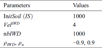
A directed acyclic construction graph is configured following Martens et al. [44]. This is based on the predictor features in the input datafile. Initial parameter values are as per Tab. 1. The graph is initialized with an equal amount of soil on all edges (1000). There are 1000 IWDs and each begins its trip with zero soil  . The velocity of each IWD is 4 based on [34]. Optimal velocity is then determined experimentally. While travelling, each IWD constructs its solution, gathers soil and gains velocity.
Table 1: Initial parameter values
IWDs move through the construction graph commencing from the  vertex towards the
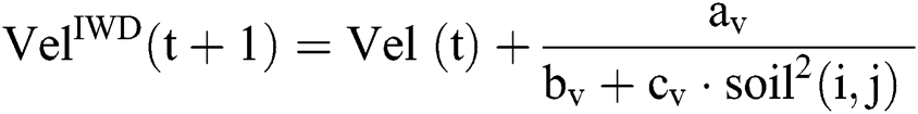
  vertex forming a rule as follows. From the current value (node) in the current vertex group (attribute), the IWD probabilistically chooses a value (node) from the next vertex group (attribute) according to the heuristic used, the velocity of the IWD and the soil available on graph edges (Eq. (1), which is also a function of Eq. (2), where
  is the list of nodes visited by this IWD,
  is used to shift
 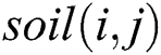 on the path joining nodes
 and
and  ).
).
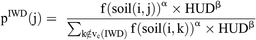
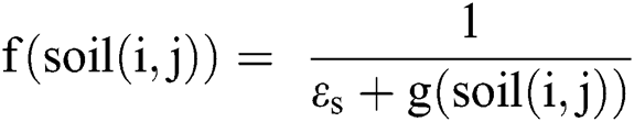
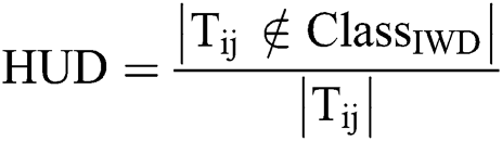
A heuristic then measures the undesirability of a move by an IWD from  to
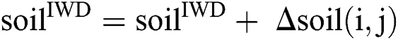
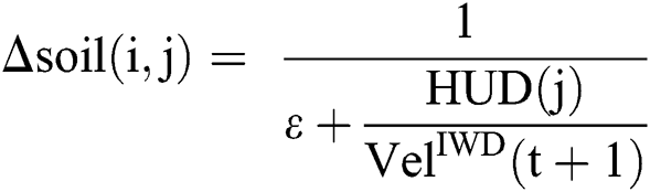
to  (Eq. (3)). Next, the IWD’s velocity (Eq. (4)) and soil (Eq. (5), which is also a function of Eq. (6)) are updated. The path with less soil will have a higher chance of being selected and the solution is constructed in a sequential coverage manner, where the data points covered by the rule are removed from the dataset as per the AntMiner+ approach [44].
where  reflects the set of remaining training instances that contain
  ,
,  represents the class that the IWD contributes to for rule extraction,
 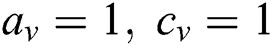 and
and 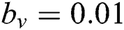 .
.
To evaluate the complete rule (solution) represented by an IWD, we follow the AntMiner+ approach [44] and use both rule confidence and rule coverage as fitness as in Eq. (7). Rule confidence is a measure of how many instances containing this specific condition belong to this class at the same time. It measures the reliability of a rule. On the other hand, rule coverage concerns how many instances in this class contain this specific condition over the total instances.
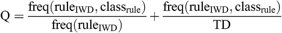
where the numerators of confidence and coverage reflect the number of rules correctly classified by this IWD; the denominator of confidence is the total number of instances covered by this IWD’s rule (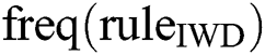 ); and the denominator of coverage is the total instances in the dataset (
 ).
).
The convergence process for solving classification problems is inspired by IWDs and AntMiner+. It aims to limit the evaluated IWDs to reach the targeted rules to complete the search faster. This is achieved when all soil in the global best path is  shown in Eq. (8) and all soil on the remaining paths is
  (Eq.(9))
where  is the number of IWDs,
  is the local soil updating parameter,
  is the global soil updating parameter,
  is the complement of
  ,
,  is the complement of
  and
and  represents the initialization of the soil.
Termination depends on many factors, including reaching the minimum convergence threshold, which represents the allowable number of convergence rules (equals 10). Termination also occurs if no water drops find a rule to cover any data instance.
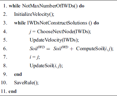
As shown in Algorithm 1, the graph is constructed in Line 1. Then, there are two main cycles: outer and inner. The initialization of the soil and the heuristic occurs on the remaining datapoints in the training set in each outer cycle in Lines 3 and 4.
Algorithm 1: Pseudocode for IWD-Miner
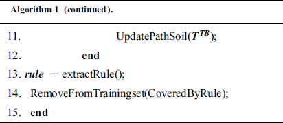
In the inner cycle, the IWDs are created in Line 6. They begin their trip at a  point and construct a solution (Line 8 of Algorithm 1 and elaborated on in Algorithm 2). This involves choosing a value from the next variable starting with
  ,
,  ,
,  and then the other variables following Eqs. (1)–(3) (Line 4 in Algorithm 2). Next, each IWD updates its velocity (Line 5 in Algorithm 2 using Eq. (4)) and soil (Line 6 in Algorithm 2 using Eq. (5) and Eq. (6)). When all IWDs are complete, the best solution is selected based on its fitness in Line 9 according to Eq. (7).
Algorithm 2: ConstructSolution(IWDs)
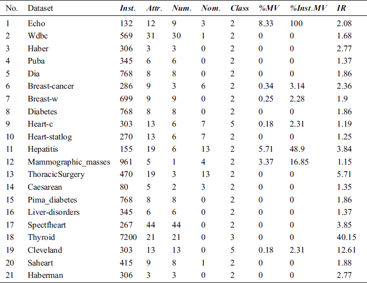
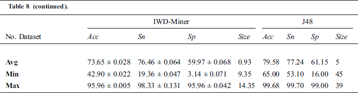
For the purposes of optimizing IWD-Miner and comparing its performance with two rival algorithms, 21 medical datasets are used (Tab. 2). These are all publicly available from the Machine Learning Repository at the Department of Information and Computer Science University of California, Irvine (UCI).  is the number of instances,
  is the number of attributes,
  are numeric attributes,
  are nominal attributes, and
  refers to the number of classes. The percentage of overall missing values (
 ) was computed as
 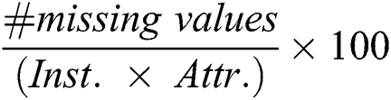 , the percentage of instances with missing values (
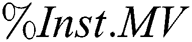 ) was computed as
  . Finally,
  is the class imbalance ratio which can be applied if the dataset contains a binary class imbalance or multi-class imbalance; there is no universally agreed threshold for the class imbalance ratio but sometimes
 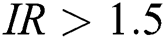 is used [46].
Table 2: Overview of the UCI datasets
Next, we used the Fayyad and Irani Discretizer as per the approach employed in AntMiner+. Finally, we used correlation-based feature subset selection which resulted in 10 features being selected.
We use standard 10-time, 10-fold cross-validation to evaluate algorithm performance with respect to each of the datasets. Five different performance criteria are used to gauge the relative efficacy of different variants of IWD Miner (Section 4) as well as the relative efficacy of the optimized IWD-Miner compared to two extant, rival algorithms (Section 5).
The first criterion is sensitivity as in Eq. (10), where  represents the number of positive records that have been correctly predicted as positive and
  refers to the number of positive records.
The second criterion is specificity as in Eq. (11), where  represents the number of positive records that have been correctly predicted as negative and
  refers to the number of negative records.
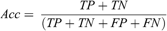
The third criterion is accuracy as in Eq. (12), where  represents the number of negative records that have been incorrectly predicted as positive and
  represents the number of positive records that have been incorrectly predicted as negative:
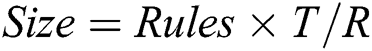
The fourth criterion is model size (Eq. (13a) for decision lists and Eq. (13b) for decision trees), where  denotes the average number of rules per individual,
  is the average number of terms per rule, and
  is the total number of leaves in a tree. Note that the measuring unit for
  is terms, while that for
  is leaves.
The fifth and final criterion is efficiency ( ) which is measured by the average number of evaluations needed to find a solution in successful runs, undefined when a solution is not found. The measuring unit for AES is fitness evaluations.
In what follows IWD-Miner is subjected to a four-stage sensitivity analysis. The best performing model from each stage is taken forward to the next stage in a process of sequential optimization.
4.1 Stage One: Path Update Procedure
First, we compared two models:  and
and  (Tab. 3). The former only updates the soil path of the best IWD (Algorithm 1, Line 11) and as such does not consider the soil update between adjacent vertexes (Algorithm 2, Line 8). The latter updates the soil paths of all IWDs and chooses the best performing model. As such, the path’s soil is updated twice: first when each IWD’s selected vertex updates the path between the previous vertex and the next vertex (Algorithm 2, Line 8) and second when the path’s soil of the best IWD is updated (Algorithm 1, Line 11). In terms of the differential performance of these two models across the 21 datasets, Wilcoxon signed-rank tests did not detect a statistically significant difference between the two models in terms of
  (p = 0.986),
  (p = 0.765),
  (p = 0.768) or
  (p = 0.375). However, there was a significant difference between the two models as measured by
  (p = 0.001), where
  had the performance advantage. Accordingly,
  is taken through to the next stage.
Table 3: Optimisation: path update procedure
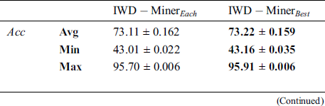
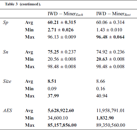
The superior performance of  with respect to
  can be understood in the following terms. As IWDs are affected by each other, updating the soil path of each IWD increases the probability of choosing the same path by the next IWD, which means producing a large number of duplicate rules. Hence, a small number of unique rules will be evaluated after the filtering step. Considering performance with respect to the properties of the datasets,
  had a better AES in most datasets featuring high imbalance ratios (
 ) such as wdbc, haberman and saheart. Moreover, the best Max
  value was associated with the thyroid dataset, which has the largest number of instances and the highest IR. Furthermore, for most datasets with missing values (%MV) and instances with missing values (%Inst.M,)
  had better AES. Examples include the breast-cancer dataset, mammographic-masses dataset and heart-c dataset. In sum, as
  ,
,  , the number of instances and
  increase so does the relative performance of
  compared to
  in terms of the
  criterion.
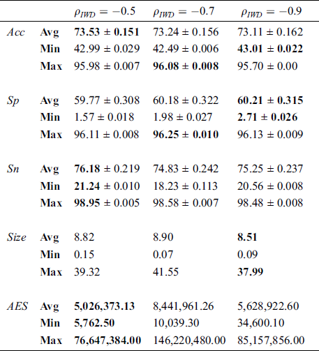
4.2 Stage Two: Global Soil Updating Parameter
Next, we experimented with three different values of the global soil updating parameter  : −0.5, −0.7 and −0.9 (Tab. 4). Similar to what was observed above in stage one, these three models performed similarly well across the 21 datasets. Friedman tests did not detect statistically significant differences in performance in terms of
  (
( = 0.172),
  (p = 0.538),
  (p = 0.495) or
  (p = 0.827). However, there was a significant difference between the three models as measured by
  (p = 0.000) with
  = −0.5 having the performance advantage. Accordingly,
  (stage one) with
  = −0.5 (stage two) is taken forward to stage three.
Table 4: Optimization of global soil updating parameter
4.3 Stage Three: Number of IWDs ( )
)
Here our purpose is to explore the impact of the number of IWDs ( ) on model performance. We compared the performance of four model variants across the 21 medical datasets. Specifically, we explored the ramifications of 500, 750, 1000, 1250 and 2000 IWDs (Tab. 5). Interestingly, no significant differences in performance were revealed across the five models with respect to any of the performance criteria according to Friedman tests: Acc (p = 0.785), Sp (p = 0.394), Sn (p = 0.938), Size (p =0.450) and AES (p = 0.349). Accordingly, we retain the default value of 1000 IWDs.
Table 5: Optimisation: number of IWDs
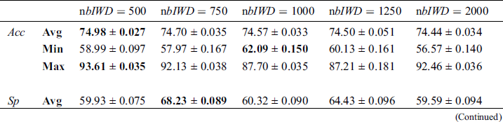
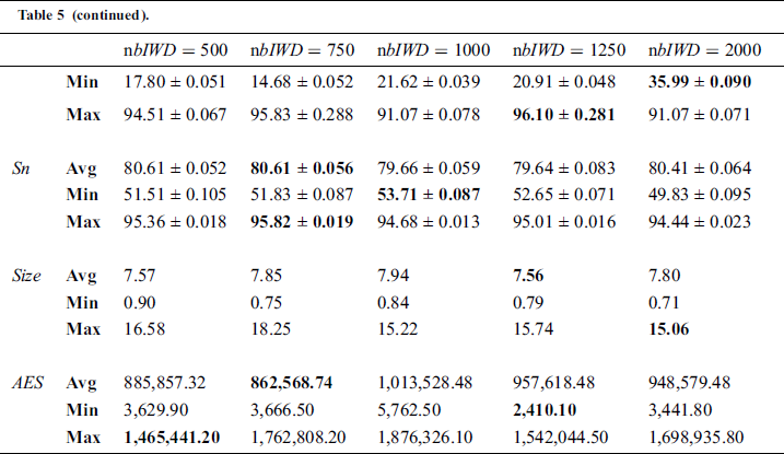
The revealed insensitivity of the algorithm in this respect can be understood in the following terms. IWD-Miner filters duplicate rules so that only unique rules are left; varying the number of IWDs impacts on the number of rules but not the number of unique rules.
4.4 Stage Four: Initial IWD Velocity ( )
)
Finally, we explore the impact of alternative initial IWD velocity ( ) values. Again, leveraging the 21 medical datasets, we compared the model where
  = 4 with three models where
  = 0, 8 and 10 (Tab. 6). Friedman tests did not detect statistically significant differences between the four models in terms of
  (p = 0.440) and
  (p = 0.113). However, significant differences were revealed with respect to the remaining three criteria:
  (p = 0.043),
  (p = 0.035) and
  (p= 0.000). The model where
  = 10 proved to be superior in terms of
  , but in terms of Sn and Acc, the model where
  = 8 performed best. We therefore opted for
  = 8 in the final version of IWD-Miner.
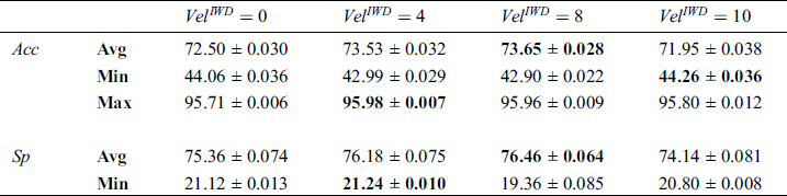
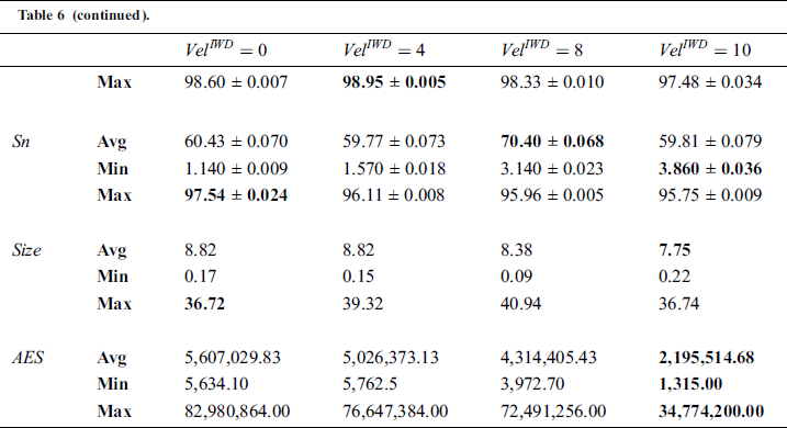
IWD velocity controls the amount of soil that will be gathered by each IWD as it moves; greater velocity leads the IWD to accumulate more soil by removing it from the path [47]. The amount of soil removed from the riverbed by an IWD during movement will affect the probability of the next IWD choosing the same path, which generates similar rules. Thus, the number of rules will decrease after applying a filtering step to retain only unique rules. This explains why a velocity of 10 proved superior in terms of efficiency but the lower value of 8 had the advantage in terms of other performance criteria.
We explored the relative performance of the optimized IWD-Miner against AntMiner+ and J48. Default settings were used for both rival algorithms, with an equal number of agents between AntMiner+ and IWD-Miner.
AntMiner+ is closely related to our algorithm and thus it seems prudent to evaluate whether and the extent to which the former can be modified in ways which have performance advantages. J48 was chosen as a comparator because it is a well-known and widely used classification algorithm which produces transparent models. IWDs is not amenable to classification problems in its original form hence its omission from this exercise.
We compared the optimized IWD-Miner with the rival AntMiner+ algorithm in terms of accuracy, efficiency, sensitivity, size of model and specificity. With the exception of efficiency, these same metrics were then used to compare IWD-Miner and J48. Efficiency is not calculable with respect to J48, hence its omission. The detailed results are shown in Tab. 7 and Tab. 8. Wilcoxon signed-rank tests did not detect a statistically significant difference between IWD-Miner and AntMiner+ in terms of  (p = 0.414),
  (p = 0.244),
  (p = 0.876) or
  (p = 0.322). However, a significant difference between the two algorithms was revealed with respect to
  (p = 0.010) with IWD-Miner exhibiting superior performance. The same non-parametric test was then used to compare the performance of IWD-Miner and J48. No significant differences were revealed between the two models in terms of
  (p = 0.986) or
  (p = 0.821). J48 exhibited superior performance in terms of
  (p = 0.04) but our proposed algorithm was revealed to have a statistically significant advantage in terms of
  (p = 0.000). Taking the breast-w dataset as an example, both IWD-Miner and J48 were comparable in terms of accuracy but the size of the former model was much smaller than the latter: 8 vs. 27.
Table 7: Performance evaluation: IWD-Miner vs. AntMiner+
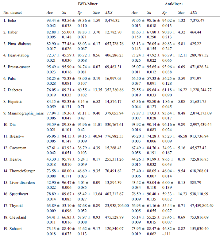
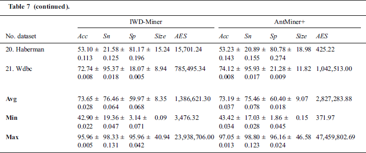
Table 8: Performance evaluation: IWD-Miner vs. J48
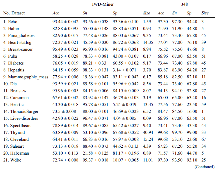
The relative accuracy of J48 could be a function of data attributes. For example, using the liver-disorders dataset, which contains 7 attributes, J48 achieved 67% accuracy compared to 43% achieved by IWD-Miner. On the other hand, using the spectfheart dataset, which contains 45 attributes, J48 and IWD-Miner achieved 73% and 93% accuracy, respectively. However, one of the strengths of J48 is the execution time it takes to build the model, which is very small compared to IWD-Miner. Another strength is its ability to handle missing values rather than eliminating records containing missing data, leading to loss of training data.
The results of the algorithm inter-comparison exercise testify to the competitiveness of IWD-Miner in comparison to two extant alternatives. IWD-Miner was shown to be as good as AntMiner+ in terms of four out of five performance criteria and better than AntMiner+ with respect to the remaining criterion, efficiency. The performance of our algorithm was comparable to that of J48 in terms of two out of four criteria; the latter was advantageous in terms of accuracy but IWD-Miner was superior in terms of resulting model sizes. As such, assuming these results generalize to other contexts (i.e., other datasets), it appears that IWD-Miner could be successfully used for the purpose of medical data classification tasks. Nevertheless, there is ample scope for future research to extend the current study in terms of algorithm development and testing. IWD-Miner takes a relatively long time to run in its current form. To mitigate this issue, we recommend exploring if and the extent to which the convergence process of the algorithm can be improved. Further, although the sensitivity analysis conducted herein suggested limited differences between IWD-Miner variants, there is scope for exploring alternative methods of discretization and feature subset selection and, finally, it may be prudent to implement a delayed procedure for handling missing values after attribute selection.
Acknowledgement: The authors would like to thank the anonymous reviewers for their constructive comments.
Funding Statement: This research project was supported by a grant from the “Research Center of the Female Scientific and Medical Colleges”, the Deanship of Scientific Research, King Saud University.
Conflicts of Interest: The authors declare that they have no conflicts of interest to report regarding the present study.
1. K. D. Boudoulas, F. Triposkiadis, C. Stefanadis and H. Boudoulas. (2017). “The endlessness evolution of medicine, continuous increase in life expectancy and constant role of the physician,” Hellenic Journal of Cardiology, vol. 58, no. 5, pp. 322–330. [Google Scholar]
2. P. Conrad. (2007). The medicalization of society: On the transformation of human conditions into treatable disorders. Baltimore, MD: Johns Hopkins University Press. [Google Scholar]
3. B. Gylys and M. E. Wedding. (2009). Medical terminology systems: A body systems approach. Philadelphia, PA: Davis Company. [Google Scholar]
4. M. J. Pazzani, S. Mani and W. R. Shankle. (2001). “Acceptance of rules generated by machine learning among medical experts,” Methods of Information in Medicine, vol. 40, no. 5, pp. 380–385. [Google Scholar]
5. I. Inza, B. Calvo, R. Armañanzas, E. Bengoetxea, P. Larrañaga et al., “Machine learning: An indispensable tool in bioinformatics,” in Bioinformatics Methods in Clinical Research, R. Matthiesen (ed.Totowa, NJ: Human Press, pp. 25–48, 2010. [Google Scholar]
6. N. Lavrač and B. Zupan, “Data mining in medicine,” in Data Mining and Knowledge Discovery Handbook, O. Maimon and L. Rokach (ed.Boston, MA: Springer, pp. 1111–1136, 2010. [Google Scholar]
7. M. S. P. Subathra, M. A. Mohammed, M. S. Maashi, B. Garcia-Zapirain, N. J. Sairamya. (2020). et al., “Detection of focal and non-focal electroencephalogram signals using fast walsh-hadamard transform and artificial neural network,” Sensors, vol. 20, no. 17, pp. 4952. [Google Scholar]
8. M. A. Mohammed, K. H. Abdulkareem, S. A. Mostafa, M. K. A. Ghani, M. S. Maashi. (2020). et al., “Voice pathology detection and classification using convolutional neural network model,” Applied Sciences, vol. 10, no. 11, pp. 3723. [Google Scholar]
9. E. M. Hassib, A. I. El-Desouky, L. M. Labib and E. S. M. El-kenawy. (2020). “WOA+ BRNN: An imbalanced big data classification framework using whale optimization and deep neural network,” Soft Computing, vol. 24, no. 8, pp. 5573–5592. [Google Scholar]
10. J. S. Chou, C. P. Yu, D. N. Truong, B. Susilo, A. Hu. (2019). et al., “Predicting microbial species in a river based on physicochemical properties by bio-inspired metaheuristic optimized machine learning,” Sustainability, vol. 11, no. 24, pp. 6889. [Google Scholar]
11. M. K. Abd Ghani, M. A. Mohammed, N. Arunkumar, S. A. Mostafa, D. A. Ibrahim. (2020). et al., “Decision-level fusion scheme for nasopharyngeal carcinoma identification using machine learning techniques,” Neural Computing and Applications, vol. 32, no. 3, pp. 625–638. [Google Scholar]
12. T. Li, S. Fong and A. J. Tallón-Ballesteros. (2020). “Teng-Yue algorithm: A novel metaheuristic search method for fast cancer classification,” in Proc. of the 2020 Genetic and Evolutionary Computation Conf. Companion, Cancun, Mexico, pp. 47–48. [Google Scholar]
13. S. AlMuhaideb and M. E. B. Menai. (2014). “HColonies: A new hybrid metaheuristic for medical data classification,” Applied Intelligence, vol. 41, no. 1, pp. 282–298. [Google Scholar]
14. N. Dey. (2017). Advancements in applied metaheuristic computing. Hershey, PA: IGI Global. [Google Scholar]
15. E. G. Talbi. (2009). Metaheuristics: From design to implementation. Hoboken, NJ: Wiley. [Google Scholar]
16. E. Aarts, J. Korst and W. Michiels. (2005). Search methodologies, G. Kendall, Boston, MA: Springer, pp. 646–651. [Google Scholar]
17. S. Kirkpatrick, C. D. Gelatt and M. P. Vecchi. (1983). “Optimization by simulated annealing,” Science, vol. 220, no. 4598, pp. 671–680. [Google Scholar]
18. P. Hansen and N. Mladenović. (2001). “Variable neighborhood search: Principles and applications,” European Journal of Operational Research, vol. 130, no. 3, pp. 449–467. [Google Scholar]
19. P. Hansen, N. Mladenović, R. Todosijević and S. Hanafi. (2017). “Variable neighborhood search: Basics and variants,” EURO Journal on Computational Optimization, vol. 5, no. 3, pp. 423–454. [Google Scholar]
20. A. K. Tanwani and M. Farooq. (2009). “Classification potential vs. classification accuracy: A comprehensive study of evolutionary algorithms with biomedical datasets, ” in Learning Classifier Systems, J. Bacardit, W. Browne, J. Drugowitsch, E. Bernadó-Mansilla, M. V. Butz et al., Berlin, Heidelberg: Springer, pp. 127–144. [Google Scholar]
21. A. E. Hassanien and E. Emary. (2018). Swarm intelligence: Principles, advances, and applications. Boca Raten, FL: CRC Press. [Google Scholar]
22. J. Kennedy. (2006). “Swarm intelligence, ” in Handbook of Nature-Inspired and Innovative Computing, A. Y. Zomaya, Boston, MA: Springer, pp. 187–219. [Google Scholar]
23. J. C. Bansal, P. K. Singh and N. R. Pal. (2019). Evolutionary and swarm intelligence algorithms. Cham, Switzerland: Springer. [Google Scholar]
24. S. Das, A. Abraham and A. Konar. (2008). “Swarm intelligence algorithms in bioinformatics, ” in Computational Intelligence in Bioinformatics, A. Kelemen, Berlin, Heidelberg: Springer, pp. 113–147. [Google Scholar]
25. R. S. Parpinelli and H. S. Lopes. (2011). “New inspirations in swarm intelligence: A survey,” International Journal of Bio-Inspired Computation, vol. 3, no. 1, pp. 1–16. [Google Scholar]
26. J. L. Deneubourg, S. Aron, S. Goss and J. M. Pasteels. (1990). “The self-organizing exploratory pattern of the argentine ant,” Journal of Insect Behavior, vol. 3, no. 2, pp. 159–168. [Google Scholar]
27. M. Dorigo and T. Stützle. (2004). Ant colony optimization. Cambridge, MA: The MIT Press. [Google Scholar]
28. D. Karaboga. (2005). “An idea based on honey bee swarm for numerical optimization. Turkey: Erciyes University, Technical Report. [Google Scholar]
29. R. Xiao and Y. Wang. (2018). “Labour division in swarm intelligence for allocation problems: A survey,” International Journal of Bio-Inspired Computation, vol. 12, no. 2, pp. 71–86. [Google Scholar]
30. M. Dorigo, E. Bonabeau and G. Theraulaz. (2000). “Ant algorithms and stigmergy,” Future Generation Computer Systems, vol. 16, no. 8, pp. 851–871. [Google Scholar]
31. G. Theraulaz and E. Bonabeau. (1999). “A brief history of stigmergy,” Artificial Life, vol. 5, no. 2, pp. 97–116. [Google Scholar]
32. O. Deepa and A. Senthilkumar. (2016). “Swarm intelligence from natural to artificial systems: Ant colony optimization,” International Journal on Applications of Graph Theory in Wireless Ad hoc Networks and Sensor Networks, vol. 8, no. 1, pp. 9–17. [Google Scholar]
33. H. Shah-Hosseini. (2007). “Problem solving by intelligent water drops,” in 2007 IEEE Congress on Evolutionary Computation, Singapore, pp. 3226–3231. [Google Scholar]
34. H. Shah-Hosseini. (2008). “Intelligent water drops algorithm,” International Journal of Intelligent Computing and Cybernetics, vol. 1, no. 8, pp. 193–212. [Google Scholar]
35. H. Shah-Hosseini. (2009). “The intelligent water drops algorithm: A nature-inspired swarm-based optimization algorithm,” International Journal of Bio-Inspired Computation, vol. 1, no. 1–2, pp. 71–79. [Google Scholar]
36. H. Shah-Hosseini. (2012). “An approach to continuous optimization by the intelligent water drops algorithm,” Procedia—Social and Behavioral Sciences, vol. 32, pp. 224–229. [Google Scholar]
37. S. Pothumani and J. Sridhar. (2015). “A survey on applications of IWD algorithm,” International Journal of Innovative Research in Computer and Communication Engineering, vol. 3, no. 1, pp. 1–6. [Google Scholar]
38. M. Dorigo. (1992). “Optimization Learning and Natural Algorithms,” PhD thesis. Politecnico di Milano, Italy. [Google Scholar]
39. B. Bullnheimer, R. F. Hartl and C. Strauß. (1997). “A new rank based version of the ant system: A computational study,” Central European Journal for Operations Research and Economics, vol. 7, pp. 25–38. [Google Scholar]
40. W. J. Gutjahr. (2000). “A graph-based ant system and its convergence,” Future Generation Computer Systems, vol. 16, no. 8, pp. 873–888. [Google Scholar]
41. T. Stutzle and H. Hoos. (1997). “MAX-MIN ant system and local search for the traveling salesman problem,” in Proc. of 1997 IEEE Int. Conf. on Evolutionary Computation, Indianapolis, IN, pp. 309–314. [Google Scholar]
42. E. G. Talbi, O. Roux, C. Fonlupt and D. Robillard. (1999). “Parallel ant colonies for combinatorial optimization problems, ” in Parallel and Distributed Processing, IPPS 1999, Proceedings: Lecture Notes in Computer Science (LNCS 1586), J. Rolim, F. Mueller, A. Y. Zomaya, F. Ercal, S. Olariu et al., Berlin, Heidelberg, 239–247. [Google Scholar]
43. R. S. Parpinelli, H. S. Lopes and A. A. Freitas. (2002). “Data mining with an ant colony optimization algorithm,” IEEE Transactions on Evolutionary Computation, vol. 6, no. 4, pp. 321–332. [Google Scholar]
44. D. Martens, M. De Backer, R. Haesen, J. Vanthienen, M. Snoeck. (2007). et al., “Classification with ant colony optimization,” IEEE Transactions on Evolutionary Computation, vol. 11, no. 5, pp. 651–665. [Google Scholar]
45. H. Wu and K. Sun. (2012). “A simple heuristic for classification with ant-miner using a population,” in 4th Int. Conf. on Intelligent Human-Machine Systems and Cybernetics, Nanchang, pp. 239–244. [Google Scholar]
46. M. Lango. (2019). “Tackling the problem of class imbalance in multi-class sentiment classification: An experimental study,” Foundations of Computing and Decision Sciences, vol. 44, no. 2, pp. 151–178. [Google Scholar]
47. G. James, D. Witten, T. Hastie and R. Tibshirani. (2013). An introduction to statistical learning with application in R. New York, NY: Springer Science+Business Media. [Google Scholar]
 | This work is licensed under a Creative Commons Attribution 4.0 International License, which permits unrestricted use, distribution, and reproduction in any medium, provided the original work is properly cited. |