DOI:10.32604/cmc.2020.012257
| Computers, Materials & Continua DOI:10.32604/cmc.2020.012257 | |
| Article |
Severity Recognition of Aloe vera Diseases Using AI in Tensor Flow Domain
1Department of IT & CS, Pak-Austria Fachhochschule Institute of Applied Sciences and Technology, Haripur, 22620, Pakistan
2COMSATS University Islamabad, Wah Campus, Wah Cantt, 47040, Pakistan
3Fatima Jinnah Women University, Rawalpindi, 44000, Pakistan
4Software Department, Sejong University, Seoul, South Korea
5Department of Computer Science, HITEC University, Taxila, 47080, Pakistan
6Department of Software Engineering, Foundation University Islamabad, Islamabad, Pakistan
*Corresponding Author: Muhammad Attique Khan. Email: attique@ciitwah.edu.pk; oysong@sejong.edu
Received: 22 June 2020; Accepted: 01 October 2020
Abstract: Agriculture plays an important role in the economy of all countries. However, plant diseases may badly affect the quality of food, production, and ultimately the economy. For plant disease detection and management, agriculturalists spend a huge amount of money. However, the manual detection method of plant diseases is complicated and time-consuming. Consequently, automated systems for plant disease detection using machine learning (ML) approaches are proposed. However, most of the existing ML techniques of plants diseases recognition are based on handcrafted features and they rarely deal with huge amount of input data. To address the issue, this article proposes a fully automated method for plant disease detection and recognition using deep neural networks. In the proposed method, AlexNet and VGG19 CNNs are considered as pre-trained architectures. It is capable to obtain the feature extraction of the given data with fine-tuning details. After convolutional neural network feature extraction, it selects the best subset of features through the correlation coefficient and feeds them to the number of classifiers including K-Nearest Neighbor, Support Vector Machine, Probabilistic Neural Network, Fuzzy logic, and Artificial Neural Network. The validation of the proposed method is carried out on a self-collected dataset generated through the augmentation step. The achieved average accuracy of our method is more than 96% and outperforms the recent techniques.
Keywords: Plants diseases; wavelet transform; fast algorithm; deep learning; feature extraction; classification
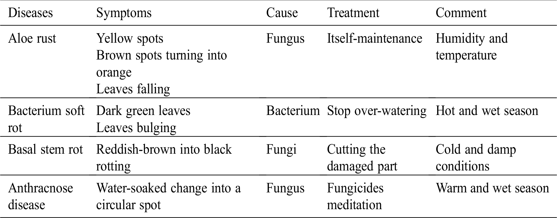
Agriculture plays a vital role in the national economy of all countries because approximately 70% of a state economy is depending on cultivation. However, plant diseases badly affect the quality of food, production, and ultimately the economy. Nowadays, Aloe vera is considered as the most famous plant in the industrial and medical fields. Aloe vera leaf gives gel that is used in medicine and cosmetics at large scale. This usage is observed more significant for cures like weight loss, inflammation, diabetes, cancer therapy, hepatitis, inflammatory bowel diseases, high cholesterol, asthma, osteoarthritis [1], stomach ulcers, insect bite, cosmetics industries, medicine industries, fever, general tonic, skin problems, hair problems, and radiation-related skin sores [2]. Aloe gel has a chemical called “acemannan,” It is used mainly for the treatment of AIDS. Consequently, the farmers are more focused on its growth and try to improve its production. However, most of the plant damage is arose due to severe diseases that cause the decrease in its production. The primary Aloe diseases of leaves are rust, Aloe rot, bacterium soft, root rot, soft rot, tip dieback, and Alternaria leaf spot. Rust is noted as a common disease in a plant. This is found on ripe plants in terms of fungal and its symptoms are shown initially on the lower surface of leaves. Anthracnose is diagnosed as a seed-borne disease that causes the death of early bright and regular seed. Soft rot occurs as a fungal disease. Macrophomina phaseolina is observed as the primary cause of fungus which can easily damage a crop in its initial stage of flowering and vegetative growth. The diseases, their causes, symptoms, and treatments are described in Tab. 2. In this regard, early identification of diseases helps to avoid crop losses and results in a better quality product. Thus, it is important to get its curing at its initial stage. In the past, agriculturists used to detect diseases in plants through manual methods. In the present era, automated methods have been performing this job [3] using machine learning models [4], image processing [5], IoT, and advanced deep learning algorithms [6]. In this regard, Pujari et al. [7] proposed the methodology for automatic disease recognition.
The feature extraction is known as the main step in machine learning. Many researchers are working on this technique for classification methods of apple, cucumber, pomegranate, and banana cultivation. Although feature extraction improves the accuracy of results in some cases, few of those features may reduce the overall accuracy. The process of feature extraction includes local binary patterns (LBP) [8], color features [9], complete local binary pattern (CLBP) [10], texture features [11,12], and histogram template feature [13,14]. Exploiting these features, classifiers are appliedusing support vector machine (SVM), decision tree (DT), and neural network (NN). This helps out to achieve the best accuracy in results [15,16].
The automatic diagnosis of plant diseases is measured as a crucial part of plant pathology. This research work intends to create a disease detection layout that is based on the Aloe vera plant observation in the machine learning domain. However, removing the noise from the digital images and detecting an exact disease part is demanded. Noise is stated as an irregular pattern of diseases like rust, rot, bacterium soft, and low contrast. This may affect the accuracy of the results. Thus to select the best classifier for feature extraction, it is asserted to improve the accuracy of results. According to [17], in any automated detection system, selection of best features improves the recognition accuracy. To realize the intended work, it is presented the overall architecture of the disease classification system that follows the image processing techniques [18,19]. These systems are typically based on three phases; image pre-processing, feature extraction, and classification [20]. In the current era, CNNs is proved that they are the best technique for image classification [21]. Many researchers have used this methodology for classification. In [22] CNNs are used to distinguish between healthy and diseased leaves of cucumbers. They diagnosed the two different diseases of cucumber using 800 images (some are captured and some are gained using data augmentation) of cucumber leaves. Another researcher is utilized the CNNs for plant leaves classification and used the public dataset [23]. They also enhanced the dataset by using an augmented process to minimize the overfitting problem in the training process. The method in [24] proposed the three different versions of the dataset: 1) red, green, blue (RGB) images, 2) grayscale images, and 3) segmented leaves. They have used two different architectures GoogLeNet and AlexNet. For automatic recognition and classification of diseases in apple leaves, nutritional deficiencies [25] used CNNs [26]. A few images are shown in Fig. 1. Tab. 1 presents the chemical composition of gel.
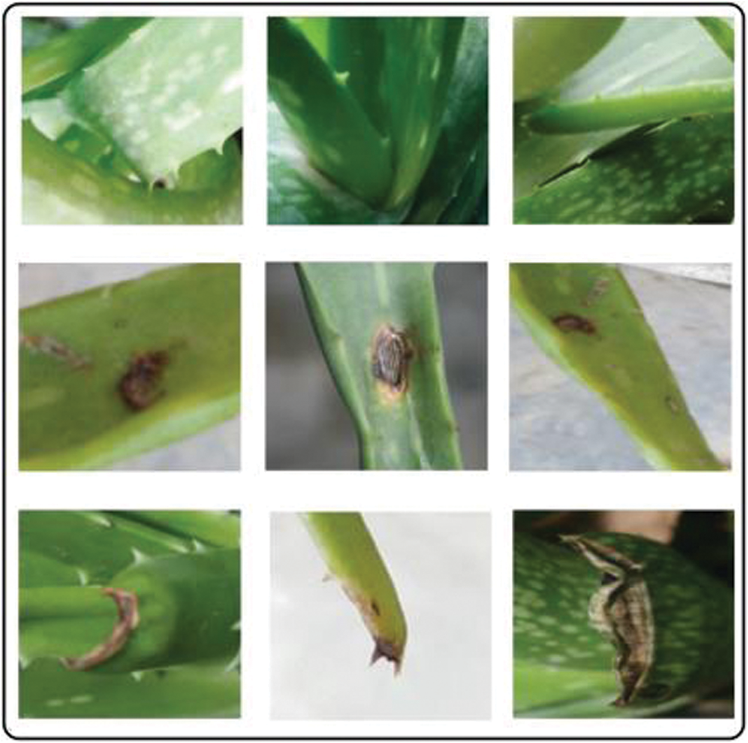
Figure 1: Samples of Aloe vera leaves: (Left to right, top to bottom), the first row shows the healthy leaves, the second row shows the rot leaves, and the third row shows the rust leaves, respectively
Table 1: Aloe vera gel characteristic composition [27]
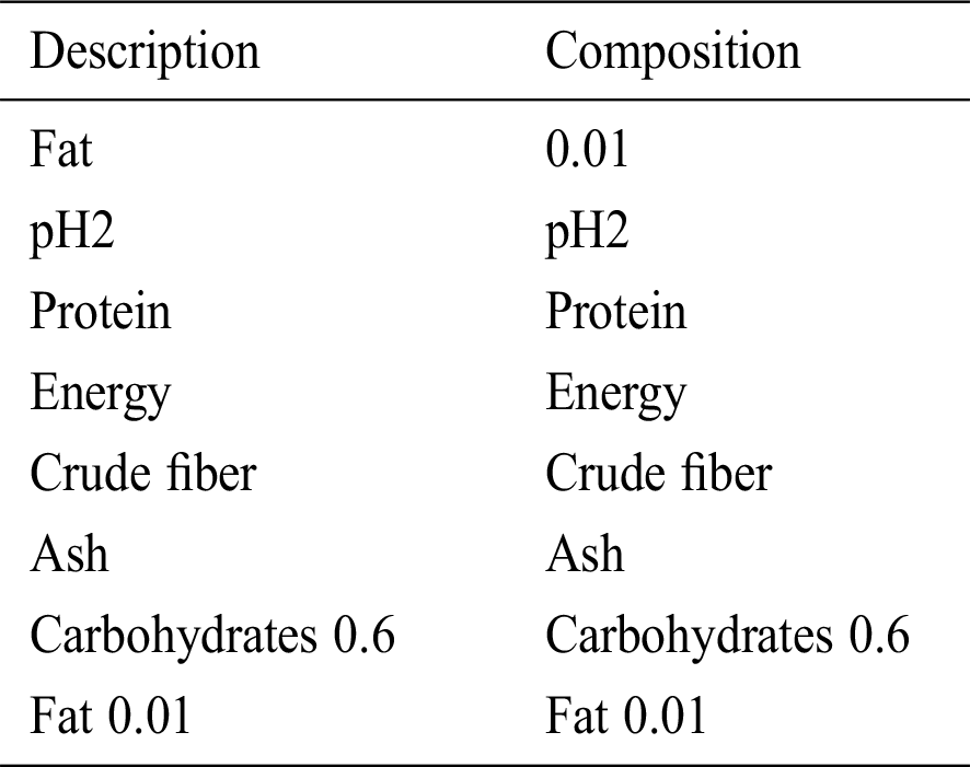
Table 2: Diseases of Aloe vera
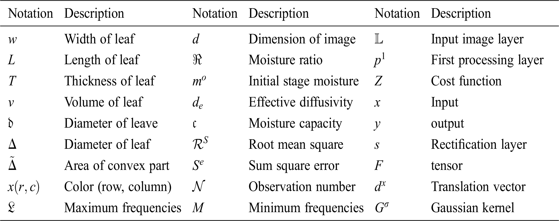
To accomplish the task of plant leaf disease detection, we use the deep learning approach in the wavelet domain. Important mathematical notions are stated in Tab. 3.
Table 3: Mathematical notions with description
First of all the Aloe vera leaves dataset is processed, as shown in Fig. 2. For the pre-processing CNNs model is used for the extraction of features using: AlexNet, VGG19, and handcraft. Aloe vera leaf, shape, and size are dependent on its length, thickness, and width. Therefore, we record several values of length that are remained in the maximum range from 60 to 100 cm. Later, we determine the dimension by using width w, length L, and thickness T of Aloe vera leaves [28] and it is found the least count values of 1 mm using the metallic scale.
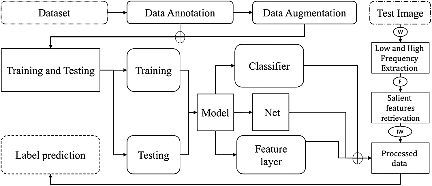
Figure 2: The proposed deep learning-based architecture for the classification of Aloe vera and Apple diseases
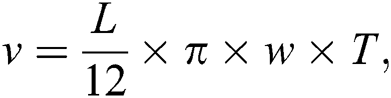
The method in [29] is defined for equating the lateral cross-section and longitudinal of Aloe leaf. It is measured the shape and volume from the given formula:
Furthermore, the diameter  of the Aloe leaf using,
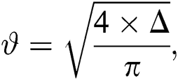
where  represents the area of the leaf. A convex-shaped image has a binary pattern that identifies the convex polygon of the image pixels. This is used for finding the convex solidity of the image. It can be demonstrated as follows:
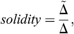
Here  show the area of convex part of the leaf. As we know, any convex binary pattern having eccentricity represents the conic section, so we calculate the eccentricity for the convex part of a leaf, and the color of any leaf can be determined using the mean and standard deviation. It can be calculated as


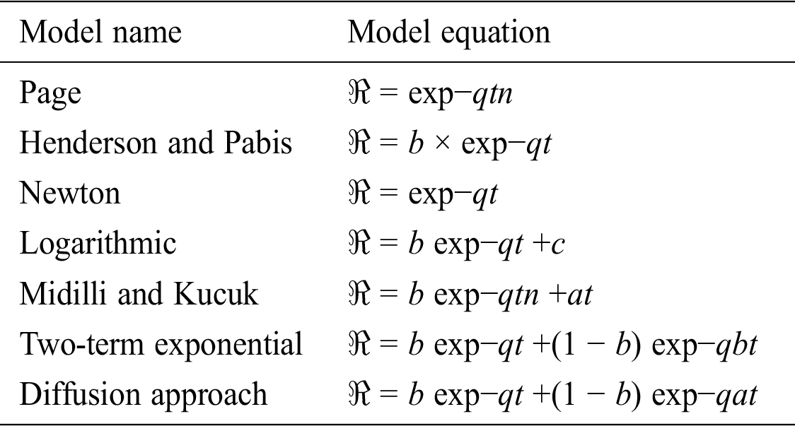
where x(r, c) is color values on row and column and d tells the dimension of an image. Using the moisture ratio , the moisture part of a leaf is described. Different model like the page and Henderson-pabis model, newton model, exponential, and logarithmic are used for briefing the leaf slices, and curve equation of drying leaf. Moisture ratio is defined as:
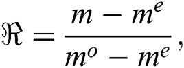
where,  shows the stable moisture, mo represents the moisture at the initial stage, and m moisture ratio at time t. Mathematical modeling of drying leaf can be explained in Tab. 4 a, b, c, where n and q are termed as constant. Using the Ficks second law for drying behavior of leaf moisture in terms of an equation, it can be written as follows:
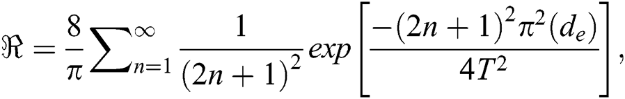
Table 4: Mathematical modeling of drying leaves
In the above equation, de is described effectivly for diffusivity (m2/s) and  half-thickness of the leaf. Ficks second law creates the relation between as a dependent variable and relates the moisture gradient with original time. Eq. (3) by [30] can be written in a semi-logarithmic form as:
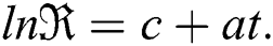
Here c is shown the carrying capacity of moist and a is demonstrated an arbitrary constant that varies with respect to t time.
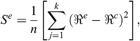
The best quality of the curves of the drying leaf model is calculated using the root mean square ( ), sum square error (
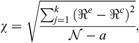
 ), and chi-square (χ); these are defined as:
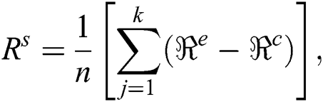
where,  is used to find the difference among the observed values and predicted values rate:
  and
and  . Se is used to calculate the discrepancy among the estimation model and data, and
  is observation number and a is any arbitrary number constant.
  and
and  show the observed value and estimated value respectively,
  can be used to calculate the variation in the cluster.
2.2 Convolutional Neural Networks (CNNs)
CNN’s are used to achieve remarkable output in image classification, recognition, object detection, and face identification, etc. It takes an input image, process, and classifies it. Input images are an array of pixels; an image has a 6 × 6 × 3 array of RGB matrix and 4 × 4 × 3 array matrix for grayscale. Input images are also based on image resolution. It deals with 3D tensor image and mathematically, the layer is defined as:

This equation shows that how CNNs run a layer by layer forward method. Here L is the input image layer, and p1 shows the first processing layer weight parameter as all the layers process until all layers finish. Lx is the output layer, and it is estimated using CNN’s posterior probability. Z is obtained as the cost function, and it is used for finding the discrepancy between the prediction Lx and target t. A simple cost function is given by:
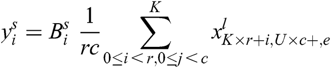
CNN’s work nicely on multilayers. 1st layer is provided the convolution layer. This layer is used for feature extraction from input images. This layer is composed of 4D tensor using CNNs. So, we can visualize the convolution process of any image by the following equation:
where r and c is a row and column kernel width respectively, E convolution output, x is input, and B convolution kernel. The second layer of this model is known as rectified linear unit (Relu). It is observed as a kind of activation function. it is used for solving the non-linear functions like sigmoid and tan functions and vanished the gradient descent. It arises when the higher layer is situated between the 1 and −1, while lower layers have a gradient approximately near to 0. This layer utilizes the simple function f (x) = max (0, xt ) and gives the value of all the input. Relu layer does not change the size of input images, f (x) = max(0, x) is not differentiable at x = 0, hence given below equation has a litter problem in theory but in practice, it works well and safe to use.
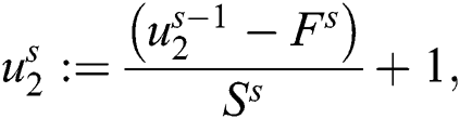
Here [x], indicates that x = 1 is true otherwise, 0. The next layer of this model is denoted the pooling layer. Suppose,  is an input pooling layer. Here l is observed as an input to the lth outer layer, r is the row, c is column and E is slices of matric. It is used for reducing the size and increase the computational speed. Pooling operation is needed no parameter but a spatial extent of pooling (r × c) is designed especially for CNNs modeling. It is observed as a matrix of input images of the given layers. Between each layer of pooling, various layers are added to solve the problem of overfitting. Finally, after the pooling of layer data, it goes to a fully connected multilayer perceptron, which includes 50 nodes of the hidden layer and two nodes of Softmax output. The final result of this layer is determined as the Softmax output layer. For keeping the model updated, weights are used as the gradient descent and conventional backpropagation (BP). For reducing the overfitting problem, we set the learning rate of about 0.001 to 0.02 in the training process, the purpose of the convolution layer is recognized as the local conjunction from proceeding layers, and they map to verify the required features. Let us suppose the local receptive and perceptron compressed in feature map with the size
 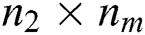 . Furthermore, every filter is applied to its position according to its volume and here
  is a filter in each layer. Every filter recognizes the feature of input images at every location. The output result
  of the layer, s contains the features
  with the size
  . The jth feature map is represented by
  and mathematically expressible as:
Here  shows the bias matrices, filter
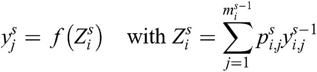
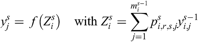
  and s is a layer of i feature. CNN’s non-linearity layer contains an activation function that generates an activation map as an output. As we know, the activation function is noted as pointwise, and the volume of input and output of the dimension is derived indistinguishable. Let any non-linearity layer s, takes
  as a features layer to the convolution layer that able to produce the activation function
  as follows:

where  is provided the size of each filter in the convolution layer. A rectification layer works as a point-wise absolute value operation. Let us take s as a rectification layer and
  nonlinear layer produce activation volume of rectified
  the properties of point-wise function do not change the input volume size correspondingly as a non-linear layer:
This function performs an important role in CNNs by abolishing the effects in succeeding layers. The next layer is rectified as a linear unit. It is designed for a combination of two layers: One is supposed as nonlinear and the other is supposed as the rectification layer. ReLU is noted as a point-wise function with thresholding at zero values:
ReLU is used for reducing the gradient descent space and likelihood problems. It is used for solving all the elimination diffculties and gives the result as sparsity activation. Sparsity is utilized for removing the noise. The next step is composed of the pooling layer. It is used for minimizing the computational cost and over the lifting of likelihood. Filter and strides are developed as two parameters of pooling layers. Their size of input volume is observed as  and it gives us output
  . By taking the s = 10 strides and the filter
  . The output of the image volume is defined:

The pooling layer is used in feature detection, image identification, and used as translational invariance. The last layer is a fully connected layer that is defined as a multilayer structure. The aim of FCL is based to connect the activation volume 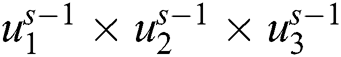 from different layers in the probability distribution.
  is defined as the output layer, where i is multilayer. We call it as activation value with input and conclusion of the connected layer as follows:
2.3 Feature Extraction by Using Tensor
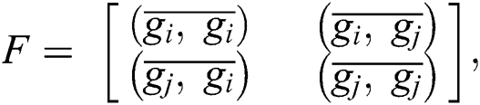
Tensor is a higher-order dimension matrix. Recently, it is used in deep learning for scheming the algorithms, features extraction of images, texture alignment, removing noise and deformation of robust, and improving the quality of images. We can define the tensor by F. Tensor defines the local orientation instead of tensor direction and equalize the clockwise rotation. Consequently, tensors are defined to describe color feature detection. Let us take an image g, then tensor defined as:
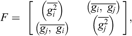
Here  shows the Gaussian filter in convolution and i, j show the spatial derivative of more than one image. We can write matric such as:
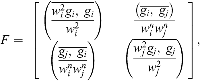
In this case, if we take g = (R, G, B), and the above equation, as a color tensor, we may assign the  and
and  as the weight functions to each measurement in
  and
and  :
:
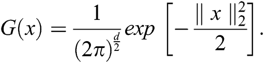
For decreasing the computational work on Matlab, we use eigenvalue analysis. Let us take an image I as pre-convolute with a Gaussian filter to improve the de-noising. Suppose for understanding, we take I = ψ and ϕ(t) = e−t/2. If I is convolute, Gaussian filter G is defined as:
For tensor, we use tensor flow basically; it is derived as a layout that describes the tensor computation program. Tensor flow is computed a numerical library. It shows the n-dimensional array of a base data type. It is developed by the Google team with the combination of neural network and machine learning researchers. Tensor flow is familiarized as an open library. It is provided a cross-platform which can efficiently run on a graphics processing unit (GPUs) and tensor processing units (TPUs), which are specially designed for mathematics work.
In machine learning, domain feature extraction is a necessary part of object recognition. The pre-trained model AlexNet and VGG19 are based on parallel methods that are used for the deep feature. Details are discussed in the following subsections.
VGG 19 consists of 19 layers with kernel size 3 × 3 matrices [31]. The input image size is 224 × 224. FC7 feature layer gives the best result as compared to other layers. Nineteen layers of VGG are used to recognize the intricate arrays within the image dataset. Max pooling is used to reduce the volume of images where a fully connected layer has 4,096 nodes that follow the Softmax classifier. It contains 140 million weight parameters. VGG19 gives the best result, but AlexNet provides the best accuracy in the result. The main architecture of VGG19 is shown in Fig. 3.
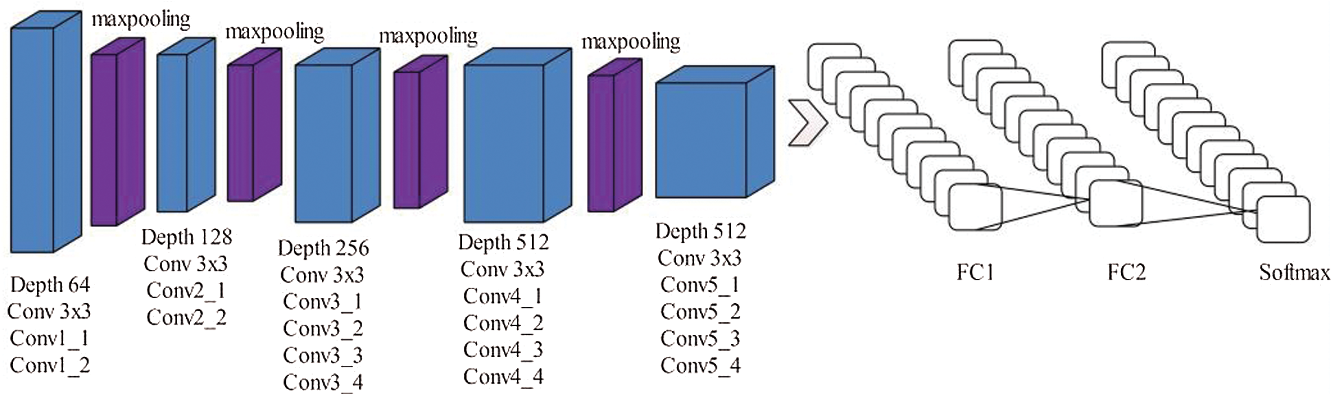
Figure 3: Original architecture of VGG19 deep neural network (DNN)
AlexNet is used as a simple CNNs structure which can be easily optimized and trained [32]. Alex Krizhevsky is designed in 2012. It consists of a total of 8 layers, the initial five layers are convolutional, and the remaining layers are fully connected. The input image size is composed on 227 × 227 × 3, and the first convolution layer has 11 × 11 filters that is applied at 4 strides and its output volume is observed about 55 × 55 × 96. The second pool1 layer consists of 3 × 3 filters, and its output volume is noted as 27 × 27 × 96. Among the last three layers, fully connected layer six (FC6) and fully connected layer seven (FC7) contains 4096 neurons and FC8 contains 1000 neurons. The original architecture of Alexnet is shown in Fig. 4.
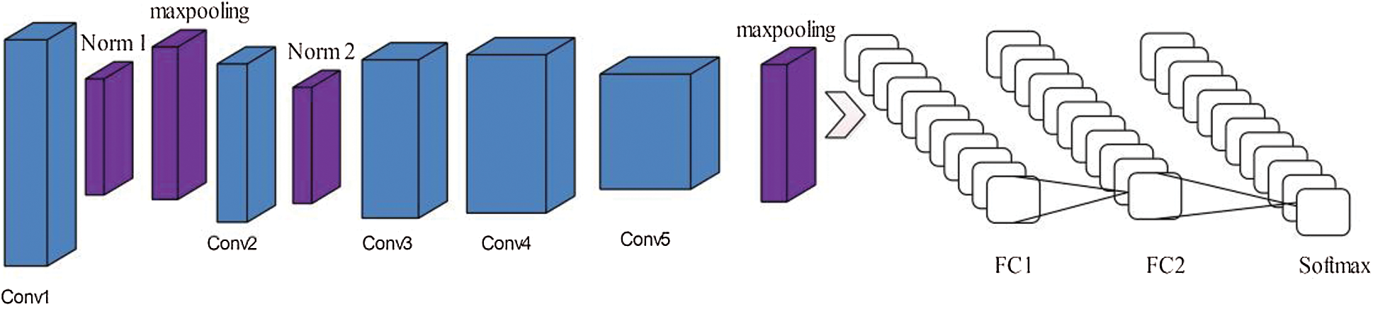
Figure 4: Original architecture of Alexnet DCNN
2.5 Feature Extraction, Fusion and Selection
Different techniques are used for feature extraction; the accuracy of any object depends on the features. Any image has features like color, shape, geometry and texture. Color is observed as the most important feature that is used for image judgment. RGB is a known model for the pretentious purpose to an image angle and light, so we must change RGB into hue, saturation, intensity (HIS) color space by using the function:
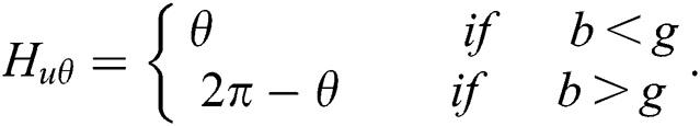
Here b and g are normalized value with the range [0, 1]. Where 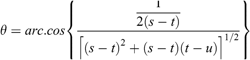 ,
,  , and
, and  .
.
Here, represents the saturation value and I is based on the intensity value of an image. Visual patterns define the texture of any image, visual recognition can be done by a 2-D deviation of grayscale.
Here φ(y) is defined for mother and φ(n,m) is defined for daughter wavelet.
2.6 Wavelet Sub-Band Replacement
During the salient enhancement process, there may occur a loss of vital information related to the noise of input image  , which can be improved from
  by a sub-band process. This is a replacement process that depends on the replacement of sub-band information for
  (
( contains the enhancement information with maximum frequencies) or M (M contains the enhancement information with minimum frequencies) in the wavelet domain. Indeed, wavelet coefficient manipulation develops the wavelets' design noise and ringing objects. M tends to keep minimum frequency information, until its maximum frequency of substances may be ruined throughout the Non-Local Mean (NLM) filter. Consequently, during the wavelet decomposition of maximum frequency enhances image M, maximum sub-bands frequencies are replaced by the noisy image
  . Accurately, w(M) extracts the four sub-band of the dataset at the
  resolution level given by
  ,
,  ,
,  , and
, and  . Last three sub-band dataset contains the maximum frequency and is exchanged by
  ,
,  , and
, and  . Afterward, take the inverse transformation of wavelet
  , first stage yields
  image. Correspondingly,
  tends to keep maximum frequency information; however, its minimum frequency substance may be ruined. During the wavelet decomposition of
  , the minimum frequency sub-band is exchanged by the
  . Here just
  is interchanged by
  The processed image
  yields in the wavelet domain with
  ,
,  ,
,  , and
, and  sub-bands. Afterward, the yields of inverses wavelets change the image into a new stage as
  . In the initial stage
  and
and  have to combine with the
  . The noisy image
  balances the significant information that could have been acquired out-of-area at a few points of the alternative process.
2.7 Removing the Noise Using Non-Local Image Filter
In image processing, Transmission electron cryomicroscopy (CryoTEM) is used to conglomerate more than thousands of two-dimensional images into a three-dimension modernization of the particle and basic use is removing noise (noise filtering) from signals, colored and grey 3-D images, it is a suitable filter for every type of image data. Noisy part of any image produces an affnity matrix. Non-Local-filter is used to remove noise by using the weight parameter for pixel values. Let suppose N be the noisy image and Ω be the discrete regular grid, d be the dimension and |Ω| is the cardinality of any image. Let the value of any re-stored image one, and s ∈ Ω is used to define the convex function combination:
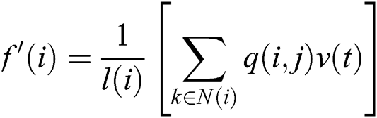
where q is the non-negative parameter, noisy image normalization constant ı(i) for any i, we have N(i) and  corresponding to the neighbor set. A parameter is used for measuring the similarity among the two square matrices (center patches); the parameter can be defined as:
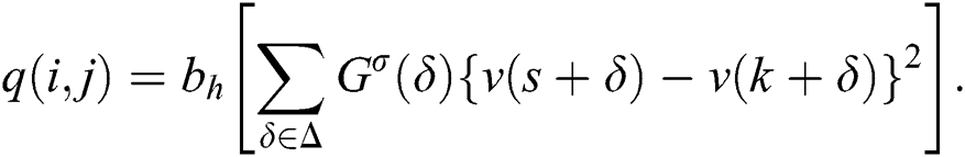
In the above equation, Gaussian kernel Gσ of variance σ, bh :  + →
+ →  + shows a non-increasing continuous function by bh(0) ≡ 1 where limx → ∞, bh(x) ≡ 0 , and δ shows the neighboring side of the discrete patch and h be the parameter which is used for the controlling amount of the filtering. Example of function bh are
  and
and  . NL-filter reinstates the image by applying the parameter weight of pixel digit values taking into account the intensity and spatial similarity. Outside pixel value does not take part in the value of f´(i). By following [33], proposed the function L(|Ω| kn pn) used for time complexity. As implemented in [34], n is the dimension of space and |ω| is the pixel value. We use the fast algorithm for filtering.
The above Eq. (36) compute the parameter q(i, j), it is a very time taking process when generating the restore data on image v. However, for one dimension to high n diminution input images, we utilized our algorithm for judgment of its accuracy. For the sake of understanding, we take ω = [0, y − 1], it shows the numbers of pixels in any image. Given dx is a translation vector and suppose an image I(dx)(n), we can define it:
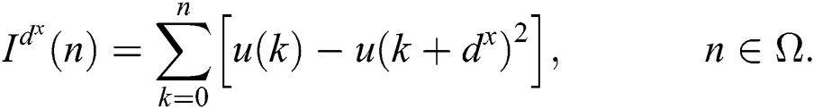
where I(dx) correlate to the image (u) and translation of image dx of different square discrete integration. When we utilized the Eq. (37), sometimes it needs to reach the outside pixel of the image. In this execution, we spread the boundary of an image in a periodic and symmetric symmetry manner to reduce memory exploitation. Our approach is to deal with two-parameters pixel value s and t. It is worth mentioning that in one dimension, images ∆ = [−n, n] represent the patches. On the opposite side, we change the Gaussian kernel with a constant value without perceptible variance. This is the main value that permits us to analyze the parameter for pixel’s couple in a unique period. Usually, a higher dimension has correlated integration with the orthogonal axis of images in the Eq. (37). We can easily see that our methodology yields a parameter calculating prescription, demanding O(2d) function for images (here d is d-dimension). The O(2d) function is independent of the patch size of the image and O(nd) function is required for each patch. Finally, the features are passed in a multi-class SVM classifier for the classification of Aloe leaf diseases. Different classification techniques are used for getting the best results like a liner, cubic, quadratic, and multiclass support vector machine (MSVM), Fine K-Nearest Neighbor (FKNN), and tree, etc. In MSVM, the given information is mapped into a nonlinear format to divide the significant information into high dimensional data for attaining the quality performance of the classification process. The support vector machine algorithm increases the margin among the classes in linearly separable cases [35]. Nevertheless, in the case where examples are not linearly separable, the kernel trick is used to transform examples to another space where they will be linearly separable. MSVM recommended results are differentiating with different classification methodologies such as linear SVM, K-Nearest Neighbor (KNN), and decision tree (DT).
This proposed method is validated on more than 7000 images of Aloe vera leaves and apple leaves. It contains three classes of Aloe and four classes of Apple leaves. Every class contains more than 1000 images. Aloe images dataset collected by Nikon D810 with the 36 megapixels, 7360 × 4921 max resolution, no optical low pass filter, and 12 bit new raw and 14-bit raw format option; whereas some images are taken by a smartphone. We also used the data augmentation technique for enhancing the images. Some collected images were normal and some had the disease. Aloe dataset consisted of three classes healthy, Aloe rust, and Aloe rot. For classification, we selected four data types apple healthy, apple black rot, Apple scab, apple rust. Healthy and diseased leaves are used for classification. We also took an apple dataset from the plant village, which has five classes. In experimental results, we used different classifier i.e., Fine Tree (FT), DT, Fine KNN (F-KNN), Linear SVM (L-SVM), Cubic-SVM (C-SVM), Multi SVM (M-SVM), Quadratic SVM (Q-SVM), ensemble boosted tree (EBT) and weighted KNN (W-KNN). Among all, MSVM gave accurate results. Apple dataset results are compared with the existing results. Experimental results are varying as if we use different features such as we chose VGG19 and AlexNet for deep architecture, dataset color, morphology, texture, RBG and grayscale parameters, selection of training-testing value, handcraft features. Results are computed using the ratio of 70, 30 along with 10 cross-validation. Five different metrics are computed from every experiment including FPR (False Positive Rate), specificity, sensitivity, precision, and accuracy. The MATLAB 2019b was used for experimental work. SVM gave the best results followed by the discrete wavelet transformation.
The proposed work is divided into two steps. The first step is disease detection from the input, which further split into stretching and extraction of diseases. We used the modified wavelet transformation and non-local filter to denoise the images and also adopted the data augmentation technique for enhancing the images. The second step is based on the classification of leave diseases of Aloe and Apple. By using the deep features, classification of healthy and unhealthy leaf images is performed and we got the best results by choosing the max pooling. For individual image classification, we used the VGG19, AlexNet, fusion, and handcraft features. In texture features, discrete wavelet transform (DWT) produced an excellent performance and the best accuracy. We also compared the apple result reported in [16], the computed results are better than [16] with 98.3% from VGG19 and 99.1% from AlexNet feature. Individual and overall results are presented in Tab. 5. In Aloe disease classification, we also classified the healthy and unhealthy samples, we obtained 95.2% from VGG19 and 96.6(%) from AlexNet. The final results of Aloe and apple are presented in Tabs. 5 and 6 respectively. Final results are obtained after 30 runs of every experiment. In the experimental work, all the best-optimized results obtained from several metrics (i.e., accuracy, sensitivity (Sen), precision (Prec), specificity (Spec), and false-positive rate (FPR)). Comparison of the proposed method with existing techniques also given in Tabs. 7 and 8, which show the effectiveness of the proposed method. Moreover, the features of the convolution layers are visualized and illustrated in Fig. 5.
Table 5: Proposed Aloe vera disease classification results
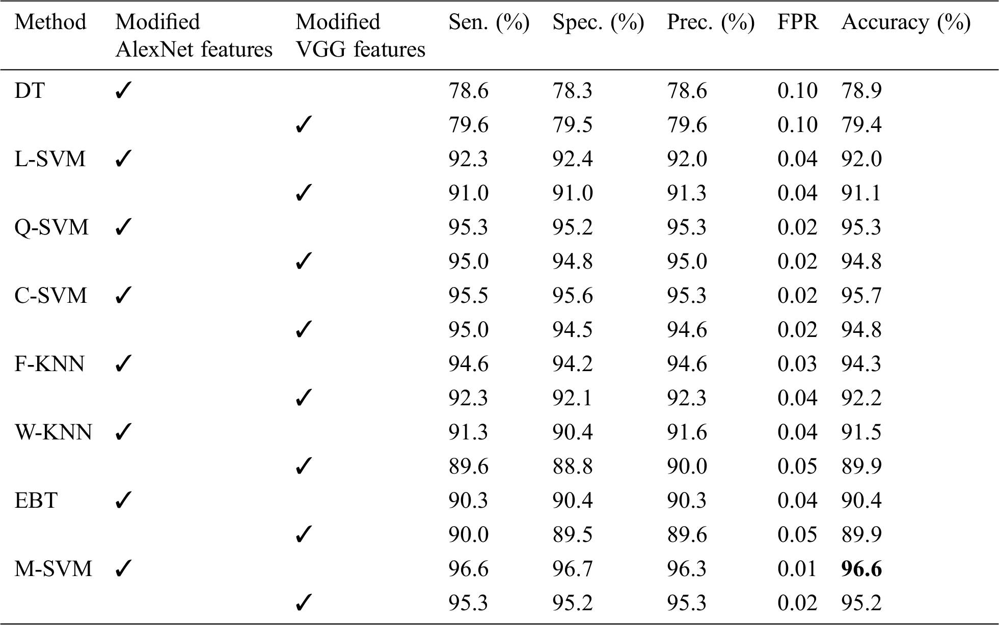
Table 6: Proposed apple disease classification results
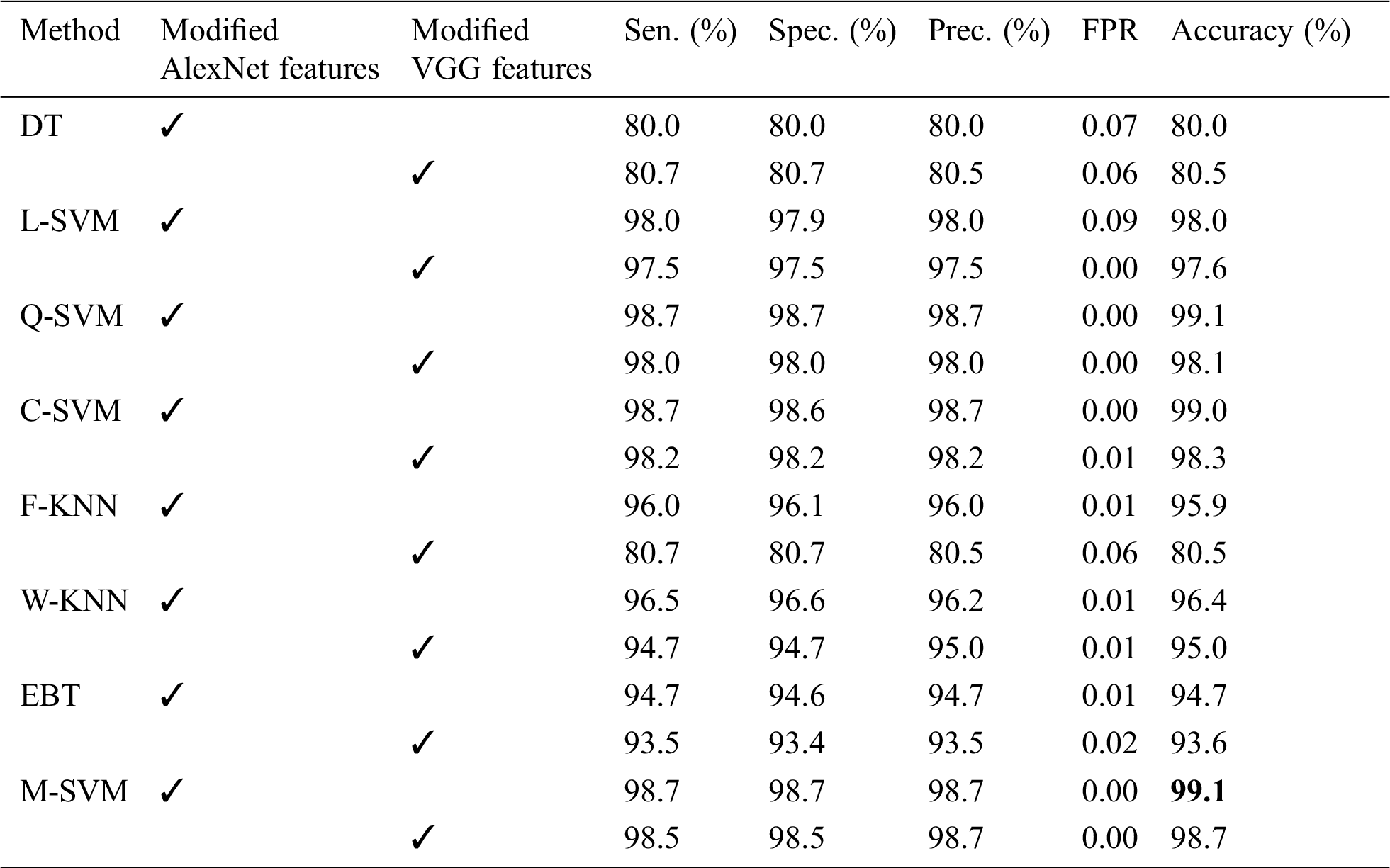
Table 7: Correlate by existing methodology
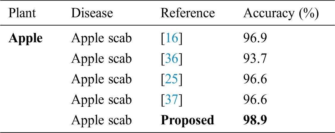
Table 8: Proposed accuracy results
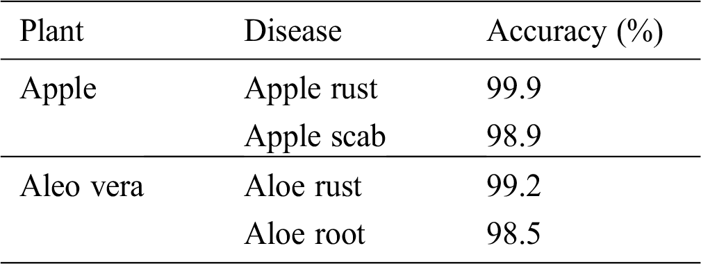
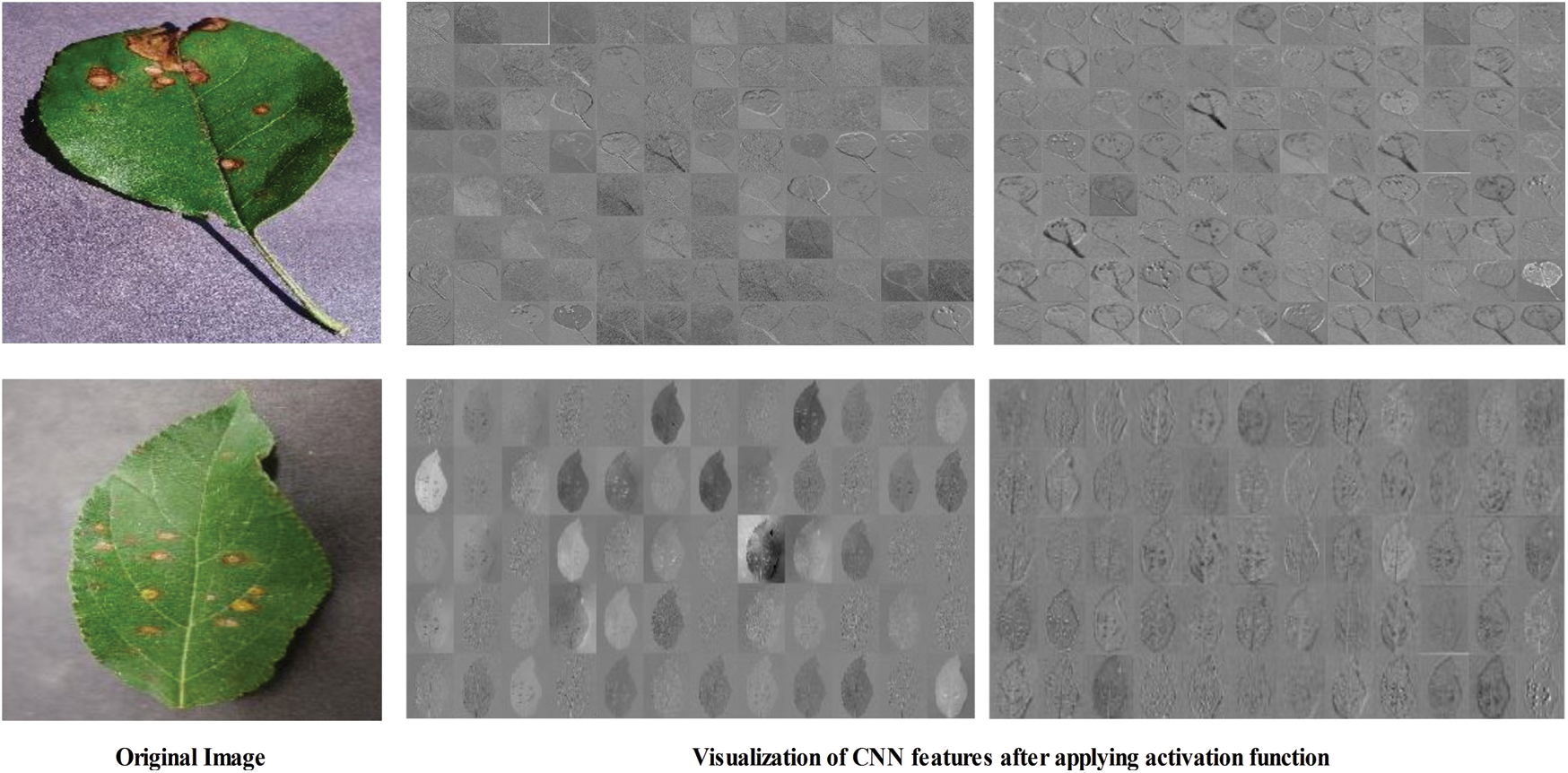
Figure 5: Features visualization after applying the activation function
In this paper, a method for disease detection and classification of healthy and unhealthy leaves using the machine learning technique is proposed. Two healthy and six unhealthy classes of diseases were classified including Aloe healthy and Apple healthy, Aloe rust, Aloe rot and Apple black rot, Apple rust, Apple rot, and Apple scab. The main focus of this research work was the classification and deep feature selection. The followed process consists of the feature extraction method, removal of the noise from the captured images, and used the data augmentation technique for enhancing the images. Removing the noise is a critical problem in any dataset; we used a non-local image filter technique to solve this problem. For classification with SVM, a non-local fast algorithm is used and found a maximum accuracy of 96.9%. The achievement in the computed results shows that the proposed methodology outperforms many existing techniques in terms of accuracy and classification. However, this research work is not without limitations which includes; i) selection of features for classification consumes more time for training; in case of the high dimensionality features, achieved good accuracy at the cost of consuming high memory and time; ii) the choice of a classifier, as the accuracy is dependent on the choice of classifier and we can not guess about the exact classifier beforehand. In the future, we intend to cover all the diseases of Aloe plant and other fruits. We further plan to modify our method for better results and low computational complexity for different diseases.
Funding Statement: This research was supported in part by the MSIT (Ministry of Science and ICT), Korea, under the ITRC (Information Technology Research Center) support program (IITP-2020-2016-0-00312) supervised by the IITP (Institute for Information & Communications Technology Planning & Evaluation), and in part by the MSIP (Ministry of Science, ICT & Future Planning), Korea, under the National Program for Excellence in SW) (2015-0-00938) supervised by the IITP (Institute for Information & communications Technology Planning & Evaluation).
Conflicts of Interest: The authors declare that they have no conflicts of interest to report regarding the present study.
1. C. Nordqvist. (2017). “Nine health benefits and medical uses of Aloe vera,” Medical News Today, pp. 34–46. [Google Scholar]
2. V. Steenkamp and M. J. Stewart. (2007). “Medicinal applications and toxicological activities of Aloe. products,” Pharmaceutical Biology, vol. 45, no. 5, pp. 411–420. [Google Scholar]
3. B. Xiong, K. Yang, J. Zhao, W. Li and K. Li. (2016). “Performance evaluation of OpenFlow-based software-defined networks based on queueing model,” Computer Networks, vol. 102, no. 6, pp. 172–185. [Google Scholar]
4. A. Adeel, M. A. Khan, T. Akram, A. Sharif, M. Yasmin et al. (2020). , “Entropy-controlled deep features selection framework for grape leaf diseases recognition,” Expert Systems, vol. 1, no. 2, pp. 1–21. [Google Scholar]
5. A. Kamilaris and F. X. Prenafeta-Boldú. (2018). “Deep learning in agriculture: A survey,” Computers and Electronics in Agriculture, vol. 147, no. 2, pp. 70–90. [Google Scholar]
6. D. Zeng, Y. Dai, F. Li, J. Wang, A. K. Sangaiah et al. (2019). , “Aspect based sentiment analysis by a linguistically regularized CNN with gated mechanism,” Journal of Intelligent & Fuzzy Systems, vol. 36, no. 5, pp. 3971–3980. [Google Scholar]
7. J. D. Pujari, R. Yakkundimath and A. S. Byadgi. (2014). “Identification and classification of fungal disease affected on agriculture/horticulture crops using image processing techniques,” in 2014 IEEE Int. Conf. on Computational Intelligence and Computing Research, Melmaruvathur, India, pp. 1–4. [Google Scholar]
8. B. J. Samajpati and S. D. Degadwala. (2016). “Hybrid approach for apple fruit diseases detection and classification using random forest classifier,” in Int. Conf. on Communication and Signal Processing, Melmaruvathur, India, pp. 1015–1019. [Google Scholar]
9. H. Qazanfari, H. Hassanpour and K. Qazanfari. (2019). “Content-based image retrieval using HSV color space features,” International Journal of Computer and Information Engineering, vol. 13, no. 10, pp. 537–545. [Google Scholar]
10. H. Zhao, Z. H. Zhan, Y. Lin, X. Chen, X. N. Luo et al. (2019). , “Local binary pattern-based adaptive differential evolution for multimodal optimization problems,” IEEE Transactions on Cybernetics, vol. 50, no. 7. [Google Scholar]
11. M. A. Khan, M. I. U. Lali, M. Sharif, K. Javed, K. Aurangzeb et al. (2019). , “An optimized method for segmentation and classification of apple diseases based on strong correlation and genetic algorithm based feature selection,” IEEE Access, vol. 7, no. 19, pp. 46261–46277. [Google Scholar]
12. M. Sharif, M. A. Khan, Z. Iqbal, M. F. Azam, M. I. U. Lali et al. (2018). , “Detection and classification of citrus diseases in agriculture based on optimized weighted segmentation and feature selection,” Computers and Electronics in Agriculture, vol. 150, no. 1, pp. 220–234. [Google Scholar]
13. H. Ali, M. I. Lali, M. Z. Nawaz, M. Sharif and B. A. Saleem. (2017). “Symptom based automated detection of citrus diseases using color histogram and textural descriptors,” Computers and Electronics in Agriculture, vol. 138, pp. 92–104. [Google Scholar]
14. H. T. Rauf, B. A. Saleem, M. I. U. Lali, M. A. Khan, M. Sharif et al. (2019). , “A citrus fruits and leaves dataset for detection and classification of citrus diseases through machine learning,” Data in Brief, vol. 26, 104340. [Google Scholar]
15. Z. Iqbal, M. A. Khan, M. Sharif, J. H. Shah, M. H. ur Rehman et al. (2018). , “An automated detection and classification of citrus plant diseases using image processing techniques: A review,” Computers and Electronics in Agriculture, vol. 153, pp. 12–32. [Google Scholar]
16. M. A. Khan, T. Akram, M. Sharif, M. Awais, K. Javed et al. (2018). , “CCDF: Automatic system for segmentation and recognition of fruit crops diseases based on correlation coefficient and deep CNN features,” Computers and Electronics in Agriculture, vol. 155, pp. 220–236. [Google Scholar]
17. H. Yu, H. Qi, K. Li, J. Zhang, P. Xiao et al. (2018). , “Openflow based dynamic flow scheduling with multipath for data center networks,” Computer Systems Science and Engineering, vol. 33, pp. 251–258. [Google Scholar]
18. A. Safdar, M. A. Khan, J. H. Shah, M. Sharif, T. Saba et al. (2019). , “Intelligent microscopic approach for identification and recognition of citrus deformities,” Microscopy Research and Technique, vol. 82, no. 9, pp. 1542–1556. [Google Scholar]
19. K. Aurangzeb, F. Akmal, M. A. Khan, M. Sharif and M. Y. Javed. (2020). “Advanced machine learning algorithm based system for crops leaf diseases recognition,” in 6th Conf. on Data Science and Machine Learning Applications, Riyadh, Saudi Arabia, pp. 146–151. [Google Scholar]
20. A. Adeel, M. A. Khan, M. Sharif, F. Azam, J. H. Shah et al. (2019). , “Diagnosis and recognition of grape leaf diseases: An automated system based on a novel saliency approach and canonical correlation analysis based multiple features fusion,” Sustainable Computing: Informatics and Systems, vol. 24, 100349. [Google Scholar]
21. M. A. Khan, T. Akram, M. Sharif, K. Javed, M. Raza et al. (2020). , “An automated system for cucumber leaf diseased spot detection and classification using improved saliency method and deep features selection,” Multimedia Tools and Applications, vol. 79, no. 20, pp. 1–30. [Google Scholar]
22. Y. Kawasaki, H. Uga, S. Kagiwada and H. Iyatomi. (2015). “Basic study of automated diagnosis of viral plant diseases using convolutional neural networks,” in Int. Sym. on Visual Computing, Springer, Cham, pp. 638–645. [Google Scholar]
23. S. Sladojevic, M. Arsenovic, A. Anderla, D. Culibrk and D. Stefanovic. (2016). “Deep neural networks based recognition of plant diseases by leaf image classification,” Computational Intelligence and Neuroscience, vol. 2016, no. 6, pp. 1–11. [Google Scholar]
24. S. P. Mohanty, D. P. Hughes and M. Salathé. (2016). “Using deep learning for image-based plant disease detection,” Frontiers in Plant Science, vol. 7, pp. 1419. [Google Scholar]
25. L. G. Nachtigall, R. M. Araujo and G. R. Nachtigall. (2016). “Classification of apple tree disorders using convolutional neural networks,” in IEEE 28th Int. Conf. on Tools with Artificial Intelligence, San Jose, CA, USA, pp. 472–476. [Google Scholar]
26. S. Zhou and B. Tan. (2020). “Electrocardiogram soft computing using hybrid deep learning CNN-ELM,” Applied Soft Computing, vol. 86, pp. 1–11. [Google Scholar]
27. K. D. Scala, A. Vega-Gálvez, K. Ah-Hen, Y. Nuñez-Mancilla, G. Tabilo-Munizaga et al. (2013). , “Chemical and physical properties of aloe vera (Aloe barbadensis Miller) gel stored after high hydrostatic pressure processing,” Food Science and Technology, vol. 33, no. 1, pp. 52–59. [Google Scholar]
28. A. Vega, E. Uribe, R. Lemus and M. Miranda. (2007). “Hot-air drying characteristics of Aloe vera (Aloe barbadensis Miller) and influence of temperature on kinetic parameters,” LWT-Food Science and Technology, vol. 40, no. 10, pp. 1698–1707. [Google Scholar]
29. S. Hazrati, Z. Tahmasebi-Sarvestani, A. Mokhtassi-Bidgoli, S. A. M. Modarres-Sanavy, H. Mohammadi et al. (2017). , “Effects of zeolite and water stress on growth, yield and chemical compositions of Aloe vera L.,” Agricultural Water Management, vol. 181, pp. 66–72. [Google Scholar]
30. P. Pisalkar, N. Jain, P. Pathare, R. Murumkar and V. Revaskar. (2014). “Osmotic dehydration of aloe vera cubes and selection of suitable drying model,” International Food Research Journal, vol. 21. [Google Scholar]
31. H. Qassim, A. Verma and D. Feinzimer. (2018). “Compressed residual-VGG16 CNN model for big data places image recognition,” in IEEE 8th Annual Computing and Communication Workshop and Conf., Las Vegas, NV, USA, pp. 169–175. [Google Scholar]
32. F. N. Iandola, S. Han, M. W. Moskewicz, K. Ashraf, W. J. Dally et al. (2016). , “SqueezeNet: AlexNet-level accuracy with 50x fewer parameters and <0.5 MB model size,” arXiv preprint arXiv: 1602. 07360. [Google Scholar]
33. Z. Guo, L. Zhang and D. Zhang. (2010). “A completed modeling of local binary pattern operator for texture classification,” IEEE Transactions on Image Processing, vol. 19, no. 6, pp. 1657–1663. [Google Scholar]
34. J. Darbon, A. Cunha, T. F. Chan, S. Osher and G. J. Jensen. (2008). “Fast nonlocal filtering applied to electron cryomicroscopy,” in 5th IEEE Int. Sym. on Biomedical Imaging: From Nano to Macro, Paris, France, pp. 1331–1334. [Google Scholar]
35. Y. Liu and Y. F. Zheng. (2005). “One-against-all multi-class SVM classification using reliability measures,” in Proc. IEEE Int. Joint Conf. on Neural Networks, Montreal, Que, Canada, pp. 849–854. [Google Scholar]
36. S. R. Dubey and A. S. Jalal. (2016). “Apple disease classification using color, texture and shape features from images,” Signal, Image and Video Processing, vol. 10, no. 5, pp. 819–826. [Google Scholar]
37. S. R. Dubey and A. S. Jalal. (2012). “Detection and classification of apple fruit diseases using complete local binary patterns,” in Proc. of the 3rd Int. Conf. on Computer and Communication Technology, Chennai, India, pp. 346–351. [Google Scholar]
 | This work is licensed under a Creative Commons Attribution 4.0 International License, which permits unrestricted use, distribution, and reproduction in any medium, provided the original work is properly cited. |